Statistical Approach to the Analysis of the Corrosive Behaviour of NiTi Alloys under the Influence of Different Seawater Environments

Abstract

Probabilistic models of corrosion rate estimation in the case of two NiTi alloys obtained by different technological processes are analysed in this paper. The depth of corrosion was measured by focused ion beam analysis on a metal surface that was not protected by an anti-corrosion coating. The samples were exposed to the influence of three different seawater environments, and empirical data were obtained in a systematic measurement procedure after 6, 12 and 18 months. Assuming that corrosion processes begin immediately after exposure of the samples to the influence of the seawater environment, and observing the corrosion rate as a random variable affected by various stochastic processes, the formed standard linear corrosion model was analysed by a statistical approach. The three best-fitted three-parameter distributions which can describe the changes in the corrosion rate for NiTi alloys exposed to the influence of the seawater environment adequately were obtained by fitting the continuous theoretical distributions. Adequate statistical tests showed similarities and differences in the behaviour of the two observed NiTi alloys from the point of view of corrosion processes caused by air, tide and sea.

1. Introduction

The possible exploitation of any material is implied by previous research of material behaviour in the environment in which it will be applied. The usage of metallic materials, especially in the complex marine surroundings, or in the environment of the sea, atmosphere, semi-enclosed and closed spaces, certainly requires numerous studies on corrosion process causes, as well as predictions of the type, extent and rate of corrosion. In this regard, there are two types of methods for predicting the corrosion of metallic materials and structural elements. The first method is based on the application of statistical models and the analysis of empirical corrosion data of metallic materials in usage. These data further represent a basis on which are calculated the mean and Standard Deviations of the corrosion rate. The second method is based on the application of a model that predicts the probability of corrosion by identifying key variables and the mechanism of the corrosion process.

Corrosion models based on a statistical analysis of large databases formed on the basis of the research of existing materials in usage, or smaller databases created on the basis of new materials, are considered the most adequate and practical in the formation of various new corrosion models. As the volume of empirical data grows (i.e., the number of samples of researched materials and collected data grows, as well as the amount of available information on exploitation conditions and influences of environmental factors), the models themselves describe the corrosion processes of the exploitation materials more realistically. The development of different corrosion models aims to understand the extent and speed of corrosion and predict the future state of materials, i.e., the technical and technological possibilities and economic justification of their further exploitation.

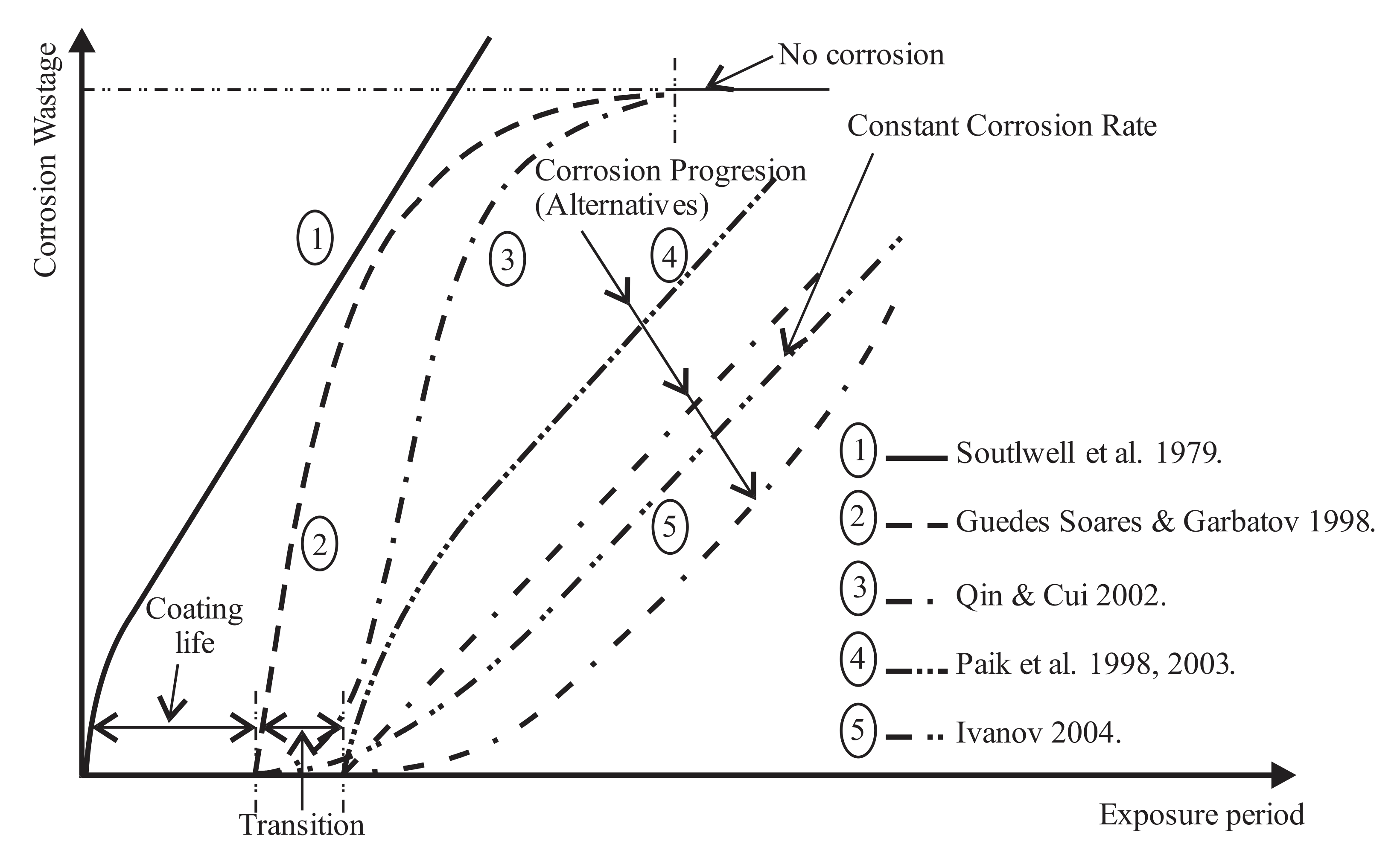
A significant number of authors believe that the corrosion process is unstable and time-dependent, and that it has a constant velocity that can be expressed linearly [1]. However, experimental evidence of corrosion published by some authors has shown that a nonlinear model is, in specific cases, more realistic in terms of describing the corrosion process. In almost all models there are two key phases during the exploitation of the material, and these are the phase of surface coating stability when there is no corrosion, and the second in which a linear or nonlinear corrosion process takes place. Whether the corrosion process will be linear or nonlinear with the slowing down or acceleration of the corrosion process depends on the environmental conditions to which the metallic materials are exposed. The environment in which metallic materials are located (dry areas, wet areas, marine conditions, changing conditions of the sea and atmosphere, etc.) influences the oxidation process of metallic materials and the intensity of the corrosion process dominantly.

One of the most important researches of corrosion processes, in which extensive databases are used, are those on ships in operation. In the past few decades, the most significant research on bulk carriers and tankers has been carried out, using databases with corrosion data detected on structures related to up to 100 ships [2,3,4,5,6,7,8,9,10,11]. The considered corrosion models describe the general and pitting corrosion of metal structural elements in a way that they can predict the degree of corrosion and the corrosion margin of individual structural elements, which was a prerequisite for the optimal design of the thickness of steel elements in operation [2,6,7,8,9].

Initially, the developed models were based on the linear dependence of the estimation of the thickness loss of steel structures due to corrosion (as suggested by Southwell et al. [12]). Lately, nonlinear models have been developed with widespread application. The most relevant nonlinear models were developed by Southwell, Guedas Soares, Paik, Melcher and others. There are also combined models that aim to reduce deviations from the empirical data that occur in simplified models. Hybrid models were developed by Qin and Cui, Ok and Pu, Melcher and others. These models are also the most acceptable models for estimating the corrosion rate, and, as such, are presented in Figure 1.

Considering the above, numerous studies and researches conducted on bulk carriers and tankers were aimed at analysing the corrosion of ship structural elements and assessing the speed of corrosion development in different environments for different types and sizes of ships. In this sense, the most significant studies are Southwell et al. [12], Yamamoto et al. [13], Ohyagi [14], Pollard [15], TSCF [16,17] and Loseth et al. [18]. The last decade has been followed by numerous studies of corrosion models, the most significant of which have been published by Gardiner and Melchers [19], Hajeeh [20], Guedas Soares and Garbatov models [21], the Paik and Thayamballi model [4,22,23,24], Qin and Cui’s model [25], Wang et al. [26], Norhazilah et al. [27,28].

While interpreting the corrosion development process (whether or not they take into account the effectiveness of the protective coating) usual corrosion models are developed as conventional models that assume that the corrosion rate has a constant value. Guedas Soares [21] and Southwell et al. [12], developed a linear, and linear/bilinear model, respectively. Yamamoto et al. [13], Guedas Soares and Garbatov [21], Paik et al. [3,4,5,6] developed a three-phase model, while Melcher developed a four-phase model [29,30] and a five phases model [31]. These phases describe the external conditions in which corrosion develops, as well as the conditions of the resulting corrosion.

Special attention is paid to the creation of unique and improved corrosion models based on the improvement of existing models, such as those in Qin and Cui [25,32], Ok [33], and Sun and Bai [34].

It is obvious that despite extensive databases and numerous models of general and pitting corrosion, there is a significant dispersion of the results of previous research. These studies cannot be considered as guidelines nor could credibly become universal models for estimating corrosion rates. The specific conditions that characterise the exploitation of metallic materials determine the degree of corrosion for each metal structure separately, and each of the presented models can only serve as a guide that directs the future user to pay more attention to certain materials during the exploitation cycle.

In the paper of Ivošević et al. [36], a statistical approach is given to investigate the corrosion rate of a CuAlNi Shape Memory Alloy. The average corrosion depths of CuAlNi alloy metal samples exposed to different seawater environments were used to determine the approximate value of the corrosion rate. In this statistical analysis, the corrosion rate was observed as a random variable represented by a linear corrosion model, based on the assumption that corrosion affects metal samples immediately upon exposure to the marine environment. Using statistical tests, the best two-parameter continuous distributions were determined, to represent the corrosion rate adequately as a random variable.

This work is organised as follows. In Section 2, the motivation of this research is presented, which is based on the analysis of the corrosive behaviour of two different NiTi alloys. This section provides an insight into the characteristics of the considered alloys from the point of view of the production process, their microstructure and physical characteristics. In addition, the methods on the basis of which empirical databases were formed are given, as well as their statistical descriptions. As the research in this paper relies on existing models of corrosion known in the literature, in this chapter a brief description of the linear corrosion model is given, which is the basis for the probabilistic model developed for the observed NiTi alloys. Section 3 provides a detailed statistical analysis of the corrosive behaviour of two NiTi alloys under the influence of different seawater environments. Within these analyses, the best three-parameter continuous distributions were detected, on the basis of which empirical data on the corrosion depth of NiTi alloys can be described adequately. Additionally, a statistical analysis was performed, which showed differences in the behaviour of the considered alloys in all three seawater environments. Concluding remarks are made in Section 4.

2. Materials and Methods

2.1. Materials

We analysed two shapes of Nitinol alloys that were produced by two different processes. Pure metals were used to produce NiTi alloys: Ni (99.99 wt.%) and Ti (99.99 wt.%) delivered by Zlatarna Celje d.o.o. Slovenia. The NiTi-1 alloy was produced by classical casting and rolling in the shape of a disc with a diameter of 42.3 mm and thickness of 3.4 mm (Figure 2a). The NiTi-2 alloy was produced by a combination of vacuum remelting and the continuous casting method. Its shape is a rod with a diameter of 11.9 mm and a length of 50 mm (Figure 2b). A total of 18 NiTi alloy samples were used for this study (nine as NiTi1 samples and nine as NiTi2 samples).

For metallographic observations all NiTi test samples were ground after electro-erosion and prepared for corrosion testing. Figure 2e,f show the different microstructures of these two NiTi alloys.

Before conducting experimental research in real environmental conditions, chemical analyses were performed by using Inductively Coupled Plasma (ICP) and X-Ray Fluorescence (XRF). Measured elements are shown in

Table 1. Chemical composition of the NiTi-1 and NiTi-2 samples.

Sample	% Ni		% Ti		% Fe
	ICP	XRF	ICP	XRF	ICP	XRF
NiTi-1	55.4	55.2–55.5	44.6	44.4–44.8	/
NiTi-2	62.6	62.5–62.6	35.9	35.9	1.4	1.4

[37].

2.2. Proposed Problem and Related Methodology

As stated in the Introduction, the deterioration of materials over time takes place depending on the type of material and the conditions in which the materials are placed, and accordingly, different linear and nonlinear models can be observed of the corrosion degradation of materials. Motivated by previous work [36,38,39,40], in this paper we explore a linear model of corrosion of two NiTi alloys. Both NiTi alloys are considered in the conditions of three specific influences of the marine environment, where the first is the constant influence of the atmosphere, the second is the constant influence of the sea, while the third influence represents the changing influences of the sea and atmosphere that take place on the sea’s surface and due to waves.

Following the described methodology, the conceptual model of the research is shown in Figure 3. The experiment is based on monitoring 18 samples of NiTi alloy (three samples of each NiTi alloy were exposed for 6, 12 and 18 months to different environmental influences). As shown in the conceptual model, all samples were placed at clearly defined locations in the boundary zone of the sea and atmosphere. Samples exposed to the atmosphere were placed near the sea but 3 m above the surface, samples exposed to the sea’s influence were immersed in the sea near the coast at a depth of 3 m, while samples exposed to the changeable influences of the ebb and flood tides were positioned on the surface.

Material characterisation by the FIB method (Focused Ion Beam on a Scanning Electron Microscope) is one of the most advanced methods for materials’ analysis. FIB instruments have both imaging and micromachining capabilities at the nanometre–micrometre scale, enhancing and enabling a broad range of fundamental studies and technological applications [36]. The research was carried out based on the characterisation of the Focused Ion Beam by measuring the depth of corrosion (in nm) on the surface of the NiTi-1 and NiTi-2 alloys after 6, 12 and 18 months of exposure. On the obtained empirical data for each observed alloy, we applied an appropriate linear corrosion model, to find the best fitted three-parameter distribution functions in different areas of the seawater environment.

2.3. Probabilistic Corrosion Rate Estimation Model

Guided by previous experience in researching probabilistic models that describe and estimate the speed of corrosion processes of ship structures [38,39,40], excellent results were obtained in our study of the corrosion behaviour of CuAlNi samples exposed to various marine influences [36], and ideas were presented in a review [25]. In this paper, we will present a statistical analysis of the analytical and probabilistic linear model applied to the assessment of the corrosion rate of two different NiTi alloys. The degree of corrosion of metal plates was characterised by the plate thickness wear ($d\left(t\right)$), which is a function of the elapsed time, so it is usually expressed by values measured in mm/years, nm/years, or nm/months [4,25]. The degree or speed of corrosion processes is influenced by numerous factors that have a stochastic nature, such as environmental conditions, type and previous state of the metal. Despite that fact, in most scientific papers, the degree of corrosion is considered a constant, resulting in a linear decrease in plate thickness over time [25]. In the works of Paik et al. [4], corrosion wear of metal plates is presented as a power function of the elapsed time. This functional dependence can be represented as follows:

$$d\left(t\right)=c_1{\left(t-T_{cl}\right)}^{c_2},\mathrm{for}t>T_{cl},$$

(1)

where $d\left(\mathrm{t}\right)$ is the corrosion wear expressed in nanometres (nm); $t$ is the exposure period; $T_{cl}$ is the service life of the coating; $c_1$ is a positive real coefficient representing the time corrosion rate, while $c_2$ is a positive real coefficient that usually takes a value of 1 or 1/3 [4].

Reference [36] confirmed the validity of Equation (1) applied to CuAlNi samples exposed to the influence of three seawater environments, air, tide and sea. The proposed model assumed that $T_{cl}=0$, resulting in $d\left(t\right)=c_{1}t$. This assumption was valid, since corrosion processes affect the degradation of sample thickness immediately after exposure to the marine environment, due to the fact that the analysed samples were not protected by anti-corrosion coating.

2.4. FIB Corrosion Depth Measurement Data Analysis

The parameters of the environment, such as temperature, pressure, salinity, particle flow rate, conductivity, etc., and their influence on corrosion processes, are not considered in this paper. Corrosion layers of both different NiTi alloys were observed with the high-resolution Scanning Electron Microscope Sirion NC400 (FEI, Hillsboro, OR, USA) with field electron emission, which enables extremely high magnifications (up to a million times) and high resolution (1 nm). It was equipped with an EDS (Energy Dispersive Spectroscopy) analyser, Oxford Instruments (Oxford Instruments, Abingdon, UK) It enables qualitative and quantitative microchemical analysis in a single point and on the surface, as well as qualitative line analysis and surface distribution of elements (mapping analysis) from beryllium to uranium. The resulting corrosion layers were evaluated and their chemical composition identified by EDS (

Table 2. Chemical composition of the NiTi-1 corrosion layers identified by EDS analysis.

NiTi-1 Chemical composition
Spectrum	In stats.	C	O	Na	Cl	Ti	Fe	Ni	Total
Spectrum 1	Yes					30.87	24.69	44.44	100.00
Spectrum 2	Yes					32.89		67.11	100.00
Spectrum 3	Yes					45.49		54.51	100.00
Spectrum 4	Yes	8.97	24.98	2.79	2.87	25.54	9.00	25.85	100.00

and

Table 3. Chemical composition of the NiTi-2 corrosion layers identified by EDS analysis.

NiTi-2 Chemical composition
Spectrum	In stats.	O	Ti	Ni	Total
Spectrum 1	Yes	4.55	37.08	58.37	100.00
Spectrum 2	Yes	4.81	37.26	57.94	100.00
Spectrum 3	Yes		46.03	53.97	100.00
Spectrum 4	Yes		44.47	55.53	100.00

).

A Quanta 200 3D electron microscope with ion beam gun—FIB (Focused Ion Beam) (FEI, Hillsboro, OR, USA) was used for measuring the depth of the formatted corrosion layer. A focused beam of primary gallium ions was enabled for etching the surface of the samples and cutting a cross-section without contamination, and, thus, gaining a direct insight into the resulting corrosion layer. Figure 4a,b show NiTi-1 and NiTi-2 samples after 12 months of exposure to the sea and corresponding FIB measuring locations. A photo view of samples with 3000 magnifications and 20 μm are shown in Figure 4c,d, while Figure 4e,f show the data on magnifications for samples, as well as corresponding corrosion depth in nm for the measured samples. All other samples of NiTi-1 and NiTi-2 exposed to the air, sea and tidal zone were scanned similarly. Figure 4g,h show the locations of the EDS analysis on the corrosion layer after the FIB cut was performed, directly on the surface and transversely in the corrosion layer. The results of the semi-qualitative EDS analysis in Table 2 and Table 3 indicate the presence of elements that are typical of corrosion products, i.e., O, C, Na and others, and differ significantly from the initial chemical composition of the investigated alloys as shown in Table 1. The electrochemical process of corrosion and uniform corrosion on the surface of the alloy was observed on the samples shown in the figures.

The number of measured corrosion depths for both observed NiTi alloys regarding three different seawater environments and after 6, 12 and 18 months of exposure, are shown in

Table 4. The number of measurements performed on each alloy in different seawater environments after 6, 12 and 18 months of exposure.

Alloy/Environment/Time		6	12	18	Total
NiTi-1	air	15	10	30	55
	tide	20	20	26	66
	sea	15	37	25	77
NiTi-2	air	22	20	40	82
	tide	25	22	32	79
	sea	24	22	29	75
	Total	121	131	182	434

.

Figure 5 and Figure 6 show all raw data of the measured corrosion depth for the NiTi-1 and NiTi-2 alloys respectively. The x-axis shows the ordinal number of measurements, while the y-axis shows the value of the measured corrosion depth expressed in nm. Data representing the depth of corrosion related to the impact of different environments (air, tide, sea) are shown in different colours, in the way described by the corresponding legends. Figure 5 and Figure 6 clearly depict the different behaviour of the alloys from the point of view of corrosion wear in the three considered environments. During the 18 months of the experiment, the NiTi-1 alloy was characterised by similar values of corrosion depth under the influence of air and tide, while the values of corrosion depth under the influence of the sea are significantly higher with a higher degree of scatter. Even in the case of the NiTi-2 alloy, the values of the corrosive influence of air are small, while the values of the depth of corrosion created under the influence of the sea are the highest. However, the NiTi-2 alloy shows significant differences compared to the NiTi-1 alloy when the tidal corrosion depth is observed. The values of corrosion depth in the NiTi-2 alloy become similar to the values of depth of corrosion created in the sea. These values increase significantly compared to the values created under the influence of air, and have much greater variability.

Table 5. Mean values and Standard Deviations ($\mu \pm \sigma$) of measured corrosion wear on the NiTi-1 and NiTi-2 alloys exposed to the influence of air, tide and sea, measured after 6, 12 and 18 months.

Alloy/Environment/Time		6	12	18
NiTi-1	air	32.75 ± 4.48	39.00 ± 43.42	53.11 ± 6.96
	tide	31.11 ± 6.08	34.41 ± 8.25	54.50 ± 7.71
	sea	48.75 ± 8.94	316.39 ± 200.88	476.17 ± 151.33
NiTi-2	air	35.80 ± 4.20	36.17 ± 4.41	58.58 ± 9.74
	tide	47.93 ± 10.52	158.02 ± 116.09	286.59 ± 190.89
	sea	144.27 ± 73.66	239.28 ± 97.55	548.02 ± 227.56

shows the basic descriptive statistics of the measured values of the corrosion depth caused by air, tides and sea, after 6, 12 and 18 months. In the first 18 months of the experiment, the NiTi-1 alloy had small values of the depth of corrosion created under the influence of air and tide. Notably higher values of corrosion wear of NiTi-1 alloys are shown after 12 months of exposure to the sea. After 12 months of sea influence, the mean value of corrosion wear of 316.39 nm was measured with a Standard Deviation of 200.88 nm, while after 18 months these values were 476.17 nm and 151.33 nm, respectively. In the case of the NiTi-2 alloy, significant corrosion processes occurred after 6 months of exposure to the sea and after 12 months of tides. Under the influence of the sea, after 6, 12 and 18 months of exposure, the mean values of corrosion depth were 144.27 nm, 239.28 nm and 548.02 nm, respectively, with corresponding Standard Deviations of 73.66 nm, 97.55 nm, 227.56 nm, respectively. The NiTi-2 alloy had mean values of measured corrosion depth of 158.02 nm and 286.59 nm, respectively, formed under the influence of the tide after 12 and 18 months. The Standard Deviation of 116.09 nm and 190.89 nm of the measured depth of corrosion caused by the tide was observed in these time intervals.

3. Results

In the process of collecting experimental data, it is not uncommon to detect data that deviate significantly from the general values of the sample. Such data that do not follow the empirical distribution are called outliers. More precisely, an outlier is an observation that lies outside the overall pattern of distribution [41]. Deviations in the measured values usually occur accidentally, due to measurement errors, or due to non-standard experimental conditions. Such data are not desirable in statistical analysis, because they can lead to poor interpretations of the results [42]. In a practical analysis of empirical data, outliers are any measurement that takes values greater than values within the width of interval 1.5 times the interquartile range above the third quartile, or below the first quartile. When applying the least-squares technique of fitting empirical data, it is recommended to remove all outliers first, to increase the statistical significance of the obtained fitted values.

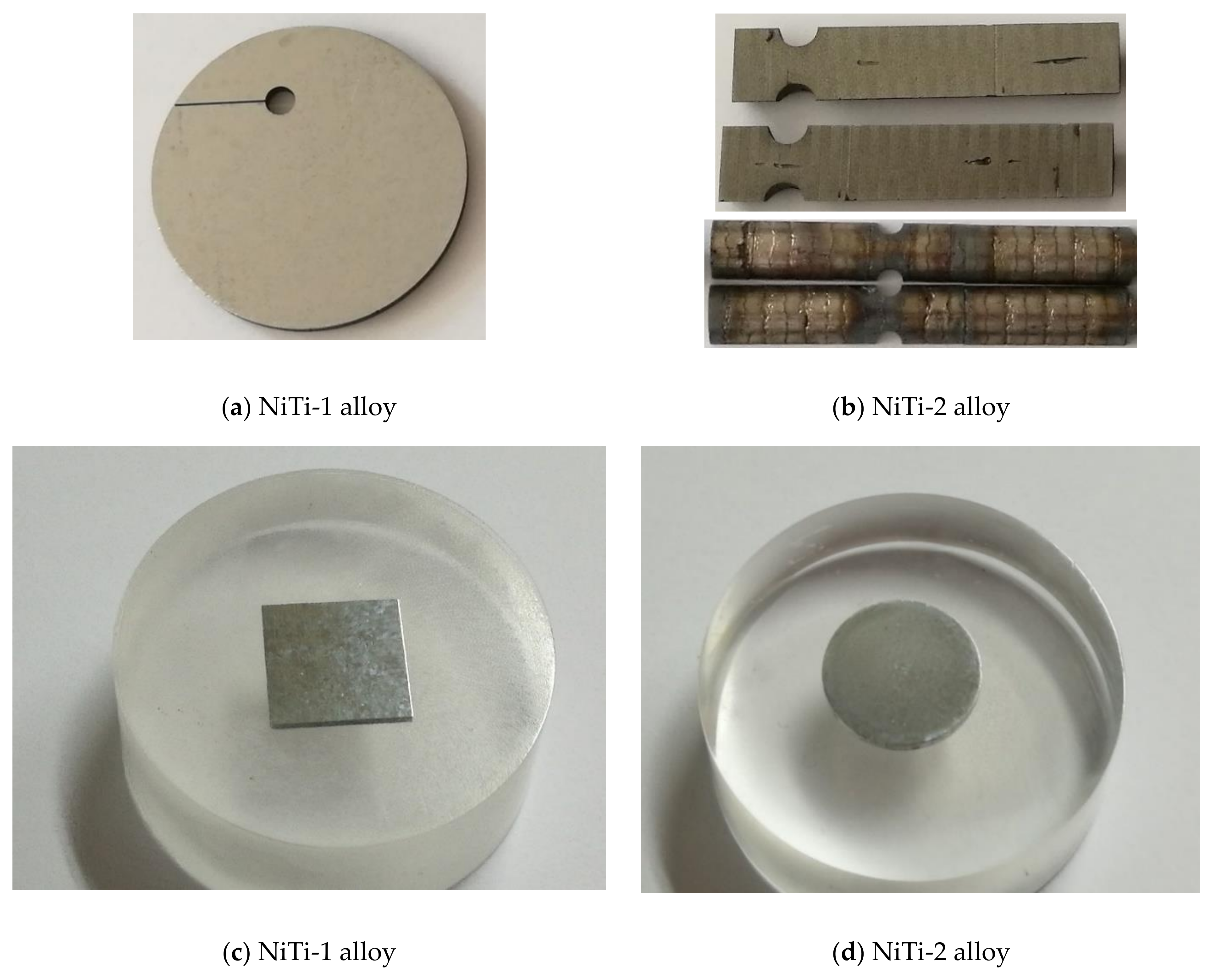
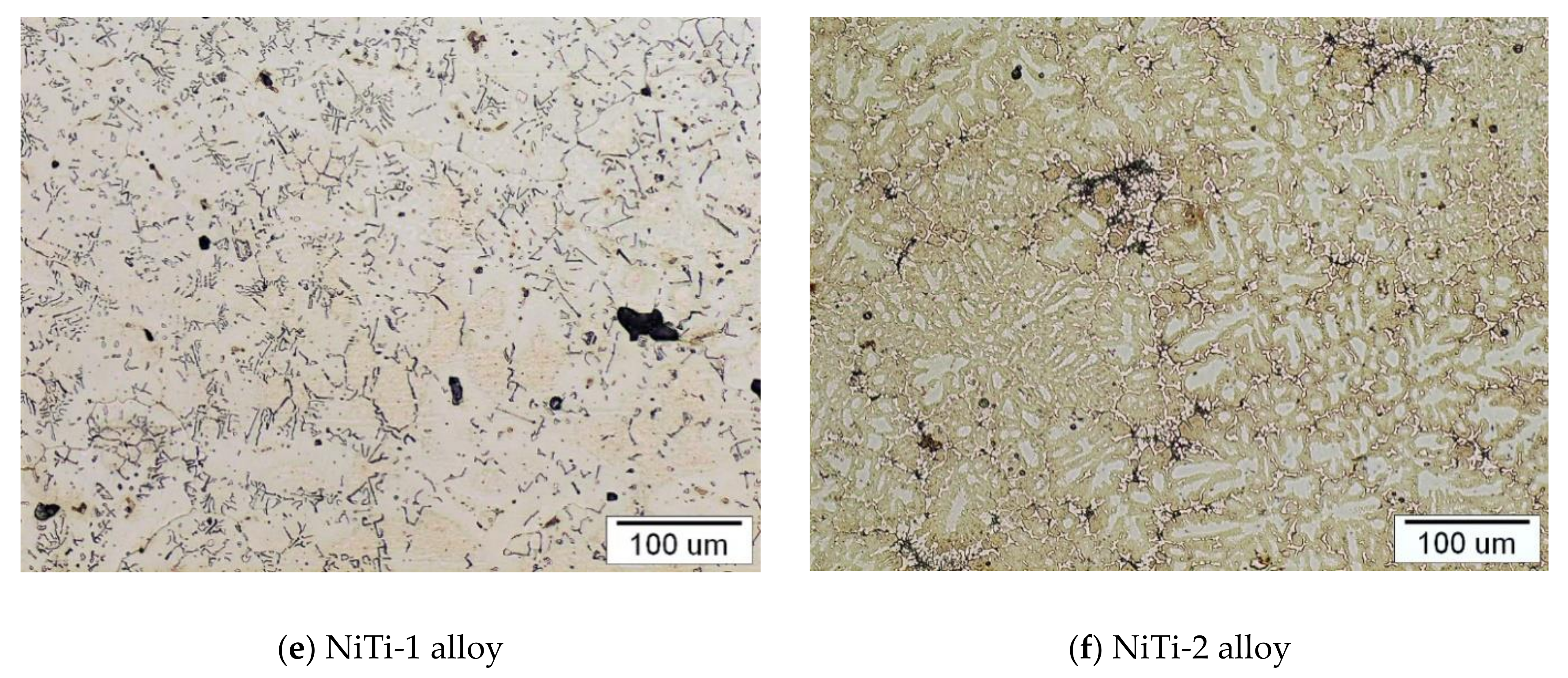
Empirical data on corrosion wear for the NiTi-1 alloy revealed 3, 6 and 8 outliers related to the influence of air, tides and sea, while for the NiTi-2 alloy 2, 7 and 3 outliers were detected for air, tide and sea influence. These data were discarded from our database after further consideration.

To interpret the depth of corrosion wear we applied a linear regression model, and thus determined the linear dependence of the corrosion wear value as a function of time. To determine the approximate values of the coefficient $c_1$ defined by Equation (1), it was necessary to calculate the mean values of corrosion wear $d\left(\mathrm{t}\right)$ at time $t$. These mean values were determined for both considered NiTi alloys and all three seawater environments. The sum of squares of the vertical offset from empirical data was minimised, to obtain the best fitted linear function to these mean values. The formed linear models for the NiTi-1 alloy are given by Equations (2)–(4).

$$d_a^{\left(1\right)}\left(t\right)=3.03036\mathrm{t},$$

(2)

$$d_t^{\left(1\right)}\left(t\right)=3.07095\mathrm{t},$$

(3)

$$d_s^{\left(1\right)}\left(t\right)=24.5832\mathrm{t}.$$

(4)

The corresponding linear models formed by the least square fitting procedure for the NiTi-2 alloy are represented by Equations (5)–(7).

$$d_a^{\left(2\right)}\left(t\right)=3.36476\mathrm{t},$$

(5)

$$d_t^{\left(2\right)}\left(t\right)=11.9605\mathrm{t},$$

(6)

$$d_s^{\left(2\right)}\left(t\right)=25.998\mathrm{t}.$$

(7)

The coefficients in Equations (2)–(7) correspond to the mean values for the corrosion rate for the observed NiTi alloy exposed to the influence of the seawater environment, and it is expressed in nm/months.

The notation $\left(x\right)$ that occurs as the exponent of the variable $d\left(t\right)$ in Equations (2)–(7) and takes values $x\in \left\{1,2\right\},$ represents the ordinal number of the observed alloy, while the notation $y$ in the index of the variable $d\left(t\right)$ that can take the value $y\in \left\{a,t,s\right\},$ represents the abbreviated name of the observed seawater environment, i.e., air, tide and sea, respectively.

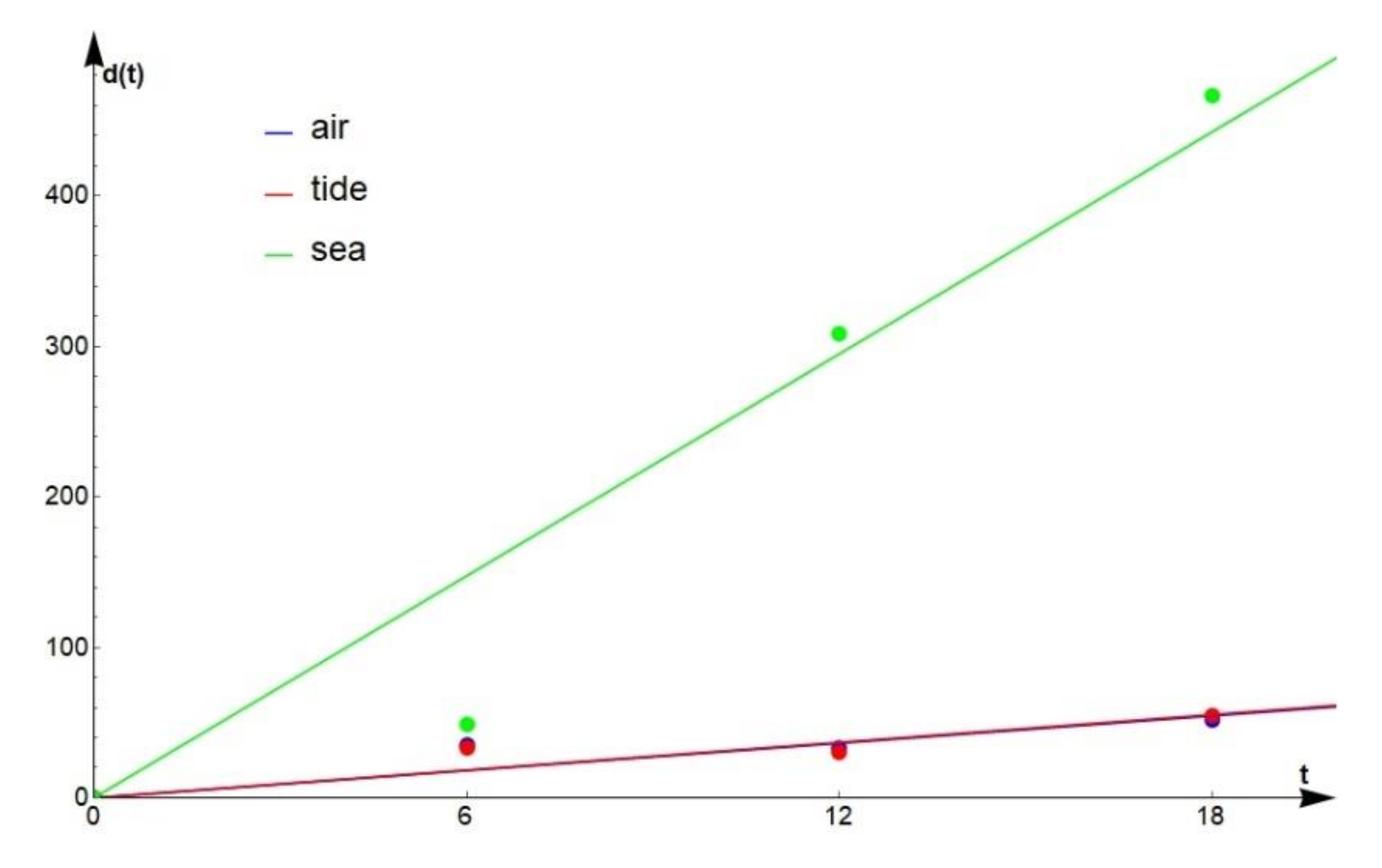
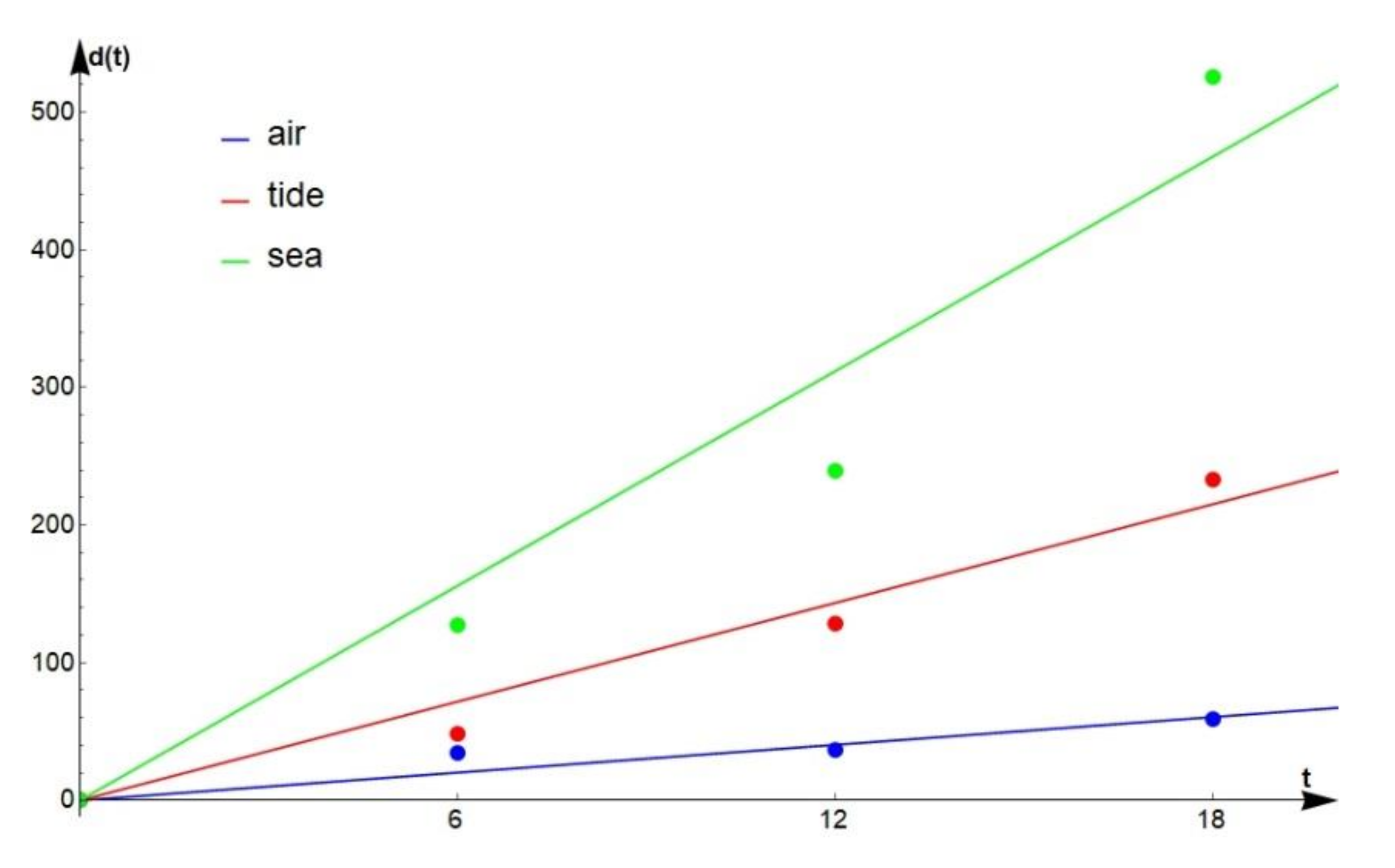
Figure 7 and Figure 8 show a graphical representation of the linear dependence of the corrosion wear $d\left(t\right)$ on the time $t$ given by Equations (2)–(7) for the NiTi-1 and NiTi-2 alloys under the influence of three different seawater environments.

Based on the visual representation of the considered linear models, it can be assumed that the NiTi-1 alloy behaved very similarly in the air and tidal environment, from the point of view of the corresponding corrosion rate values. However, this assumption should be verified further using statistical techniques.

Based on Equations (2)–(4), assuming that the monthly corrosion rate was a deterministic value, it can be concluded that the approximate values of parameters $c_1$ are equal to 3.03036 nm, 3.07095 nm and 24.5832 nm for air, tide and sea, respectively, if the considered alloy is NiTi-1. In the case of the NiTi-2 alloy, Equations (5)–(7) give approximate deterministic values of the parameter $c_1,$ which takes the values 3.36476 nm/month, 11.9605 nm/month and 25.998 nm/month, for air, tide and sea, respectively.

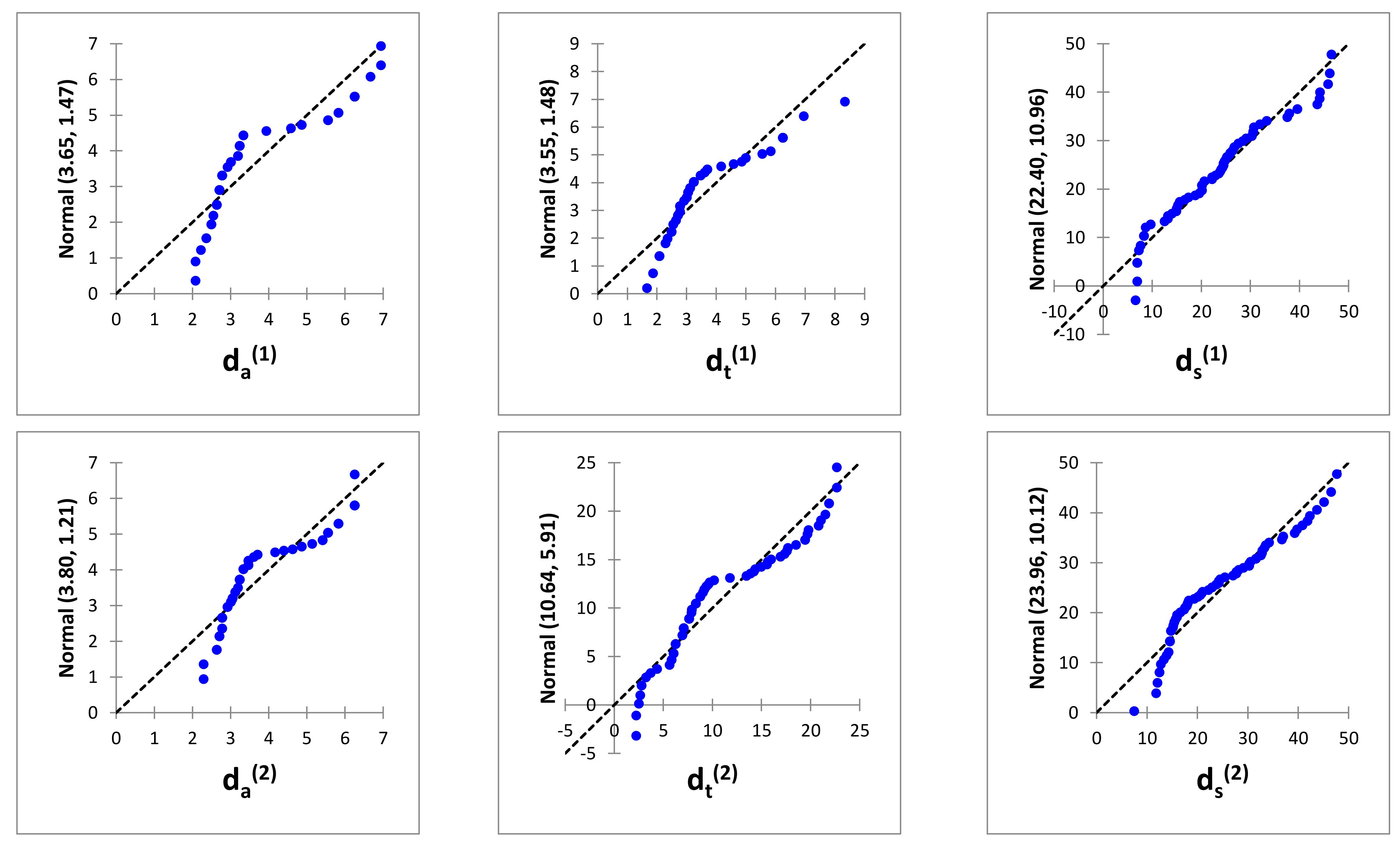
Normality tests are especially important when examining empirical data, because they direct research in the right way when choosing statistical methods for data analysis. Namely, if empirical data do not follow the Normal distribution, nonparametric tests are more suitable than parametric ones, especially if data groups are compared [43,44].

A Quantile-Quantile (Q-Q) plot was used as a graphical method of comparing the corrosion rate data sets obtained for the NiTi-1 and NiTi-2 alloys in three seawater environments with Normal distribution. Q-Q plots are graphing representations of sample order statistics against some “expected” quantiles from a standard normal distribution [43]. This graphical method is based on the fact that any significant deviation from linearity will indicate that the data cannot be characterised with a normal distribution. The obtained graphs comparing the samples with the normal distribution are shown in Figure 9. The first row of graphs shows three Q-Q plots for corrosion depth rate related to the NiTi-1 alloy in air, tide and sea environments, respectively, while the second row of graphs depicts the obtained graphical result of corrosion rate analyses for the NiTi-2 alloy in air, tidal and sea environments, respectively. Since in all six cases the pattern is not laying on the line $y=x,$ we cannot claim that our samples follow a Normal distribution.

To confirm the assumption made based on a visual examination of corrosion rate measurements, statistical normality tests were performed additionally. Normality tests calculate the probability that a sample was extracted from a normal population. More specifically, the Shapiro–Wilk normality test was chosen because of the relatively small number of observations [45]. In total, six Shapiro–Wilk tests were performed, with the null hypothesis claiming that each individual set of corrosion rate measurements followed a normal distribution. When performing the Shapiro–Wilk tests, the used hypotheses are:

H0. 

Sample data do not differ significantly from a normal population.

Ha. 

Sample data differ significantly from a normal population.

Table 6. Shapiro–Wilk test results.

	${\mathit{d}}_{\mathit{a}}^{\left(\mathbf{1}\right)}$	${\mathit{d}}_{\mathit{t}}^{\left(\mathbf{1}\right)}$	${\mathit{d}}_{\mathit{s}}^{\left(\mathbf{1}\right)}$	${\mathit{d}}_{\mathit{a}}^{\left(\mathbf{2}\right)}$	${\mathit{d}}_{\mathit{t}}^{\left(\mathbf{2}\right)}$	${\mathit{d}}_{\mathit{s}}^{\left(\mathbf{2}\right)}$
W	0.775	0.830	0.945	0.807	0.900	0.918
p-value	<0.0001	<0.0001	0.0048	<0.0001	<0.0001	0.0002

summarises the results of six Shapiro–Wilk normality tests. The first row of Table 6 shows the calculated values of the test statistics, while the second row shows the corresponding p-values. The significance level $\alpha =0.05$ was selected in all tests. As is shown in Table 6 small p-values were obtained, significantly lower than the value for α. This indicates that there was very little risk of error when rejecting the null hypothesis. The risk to reject the null hypothesis H0 while it is true is lower than 0.01%, 0.01%, 0.48%, 0.01%, 0.01% and 0.02%, respectively. Based on the results of the Shapiro–Wilk tests, it became clear that the measured corrosion rate values in all observed seawater environments for both NiTi alloys did not follow the Normal distribution.

A heavy-tailed distribution has a tail that is heavier than an exponential distribution [46], and, thus, such type of distributions converges slowly to zero. As the Q-Q graphs suggest (Figure 9), the distribution centres were well explained by the normal distributions, but the tails of the empirical data showed a tendency to deviate. Figure 9 shows that the empirical corrosion rate data had heavy tails on both sides, and are therefore not modelled well by a normal distribution. The tails of the normal distribution were too thin to produce enough extreme events to match those in the sample. In other words, the likelihood that NiTi alloys would produce a large value of corrosion rate was high. Therefore, distribution families must be considered that might represent these prominent parts better.

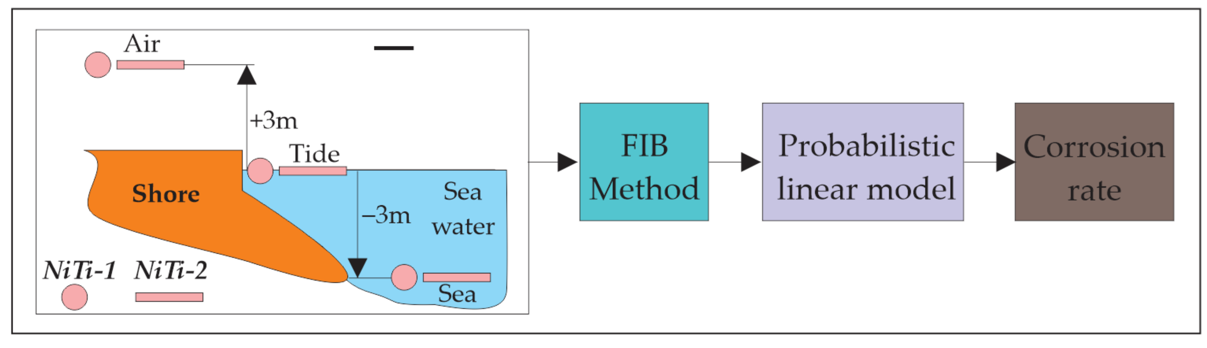
It is more convenient to consider the corrosion rate as a random variable, bearing in mind that corrosion processes are influenced by a large number of factors of stochastic nature, especially in the seawater environment [47]. A probabilistic method of fitting three-parameter continuous probability functions is proposed here, to describe the stochastic nature of the monthly corrosion rate of the observed NiTi-1 and NiTi-2 alloys in three different seawater environments.

The Probability Density Function (PDF) of a continuous function, denoted as $f\left(x\right)$, is the probability that the variate has the value $x$. The Cumulative Distribution Function (CDF), denoted as $F\left(x\right)$, is the probability that the variate X takes a value less than, or equal to, a value $x$. There is a relation between PDF and CDF of a continuous distribution: $F\left(x\right)=P\left(X\le x\right)={{\displaystyle \int }}_{-\infty }^{x}f\left(s\right)ds$, or when PDF exists $f\left(x\right)=F{\left(x\right)}^{\prime }=\frac{dF\left(x\right)}{dx}$. The empirical CDF of the sample is defined at a point $x$ as the proportion of elements in the sample that are less than, or equal to, $x$. Assuming that the x-axis is divided into intervals of equal width, the empirical PDF is defined as the quotient of the relative frequencies of the sample indices located in the observed interval and the width of the interval. For example, empirical CDFs of corrosion rate $c_1$ of the NiTi-1 and NiTi-2 alloys (denoted as $F_1\left(c_1\right)$ and $F_2\left(c_1\right)$, respectively) are shown in Figure 10. Empirical PDF for the NiTi-1 alloy can be seen in Figure 11 and Figure 12 in histogram form. Additionally, empirical CDF of corrosion rate $c_1$ of the NiTi-1 alloy is presented as a step function in Figure 13.

Three-parameter probability distribution functions are characterised by three parameters: Location, scale and shape parameter. The location parameter $p$ shifts the PDF function $f\left(x\right)$ along the x-axis by the value of $p$, i.e., $f\left(x-p\right)$. The scale parameter determines the width of the PDF function $f\left(x\right)$. More precisely, for larger-scale parameter values, the PDF function is wider. A shape parameter is any parameter that cannot describe the location and/or width of a PDF function, and cannot be represented as a function of these two parameters. Not all theoretical distributions depend on three parameters, so there are one-parameter, two-parameter and multiparameter distributions. However, in this paper, the research is focused only on the analysis of three-parameter distributions. A total of 27 different three-parameter continuous PDF functions are considered, in order to describe the stochastic nature of the corrosion rate denoted as $c_1$ best.

One of the main problems that arise when fitting theoretical distributions into empirical data is the ubiquity of oscillations in the measured values and the large variability of the data. Large changes in distribution tails produce large residuals and reduce the goodness of fit, with the result that testing statistical hypotheses becomes a highly non-trivial problem. The presented corrosion rate empirical data have a complex structure, resulting in difficulties in understanding which theoretical continuous distribution would best follow changes in empirical data. Therefore, it is necessary to examine different classes of theoretical distributions, especially those that describe well the characteristic tails of empirical distributions in different seawater environments, and, thus, increase the accuracy of the fitting.

This paper proposes a statistical approach to the analysis and approximation of the empirical CDF corrosion rate, defined by Equation (1) with two initial assumptions:

H1. 

Corrosion processes in all three seawater environments begin immediately after the alloys’ exposure to external factors.

H2. 

The corrosion rate is a random continuous variable.

Taking into account that $T_{cl}=0$ (based on the assumption a), $c_2=1,$ and applying adopted Equation (1), we obtain an adequate expression for calculating the variable $c_1$:

$$c_1=\frac{d\left(t\right)}{t},\mathrm{for}t>0.$$

(8)

By applying adequate statistical analysis to the 27 different theoretical continuous distributions, the three-parameter distributions can be detected that best describe the behaviour of alloys from the point of view of corrosion rate in different seawater environments. The probability model was developed based on the data described in Table 5 and the verification of the obtained results based on standard statistical tests.

Statistical analysis was performed by fitting three-parameter continuous distributions into empirical CDF of variables $c_1$, whose values were calculated based on the measured corrosion depths in three different seawater environments and applying Equation (8). An individual statistical analysis was performed for each of the three environments (air, tide, sea) and for each of the considered alloys (NiTi-1 and NiTi-2). In this way, the three best fitted three-parameter distributions were obtained that describe the random variable $c_1$ adequately. More precisely, a total of six groups of the three best three-parameter distributions were detected (one group was detected for each alloy in each of the three considered environments).

The process of fitting theoretical distributions begins with the selection of adequate distributions that can describe the empirical data. For this purpose, the theoretical continuous distributions characterised by the different number of parameters were analysed preliminarily. By eliminating unacceptable results due to large deviations from the empirical data, the analysis concentrated only on three-parameter distributions.

In the next phase, it was necessary to determine the optimal values of all three parameters for each of the considered theoretical distributions. The frequently applied method of unknown parameters approximation was used, known as the maximum likelihood estimation method [48,49].

Verification of the correctness of the results obtained in the previous steps involved checking the goodness of fit, and represents the last step in the statistical analysis [50]. To check the goodness of fit, i.e., to check whether the empirical data come from the reference theoretical distribution, we used two known tests from the literature: The Kolmogorov–Smirnov (KS) and the Anderson–Darling (AD) tests [51]. These two tests were selected because of their specific characteristics. The Kolmogorov–Smirnov test is a non-parametric test that does not depend on the underlying distribution, i.e., on the CDF that is being tested. The Anderson–Darling test is a more sensitive test (especially on the tails of the distribution) [52], that uses the CDF values of the observed reference distribution.

The selection of the three best-fitted three-parameter distributions, as well as their ranking, was guided by the results of the Kolmogorov–Smirnov test, while the Anderson–Darling test served for additional verification of the results. The ranking was possible based on the calculated values of the test statistics of the KS and AD tests. The lower values of the test statistics indicated the fact that the fitted theoretical distribution described the empirical data better, and therefore the observed theoretical distribution had a better rank.

The standard notations $f\left(x\right)$ and $F\left(x\right)$ for PDF and CDF, respectively [53], of the considered theoretical distributions were used in the following sections. For the sake of clarity and easier presentation of the results, to these labels were also added labels related to the seawater environment, the ordinal number of the NiTi alloy, as well as the abbreviated name of the considered theoretical distribution, resulting in terms $f_{y_z}^{\left(w\right)}\left(x\right)$ and $F_{y_z}^{\left(w\right)}\left(x\right)$, respectively. The above notation $\left(w\right)$ is an abbreviation for the considered theoretical distribution name. The notation $y$ below refers to the seawater environment (air, tide, sea) and can take one of the values from the set $\left\{a,t,s\right\}$, while the index $z$ takes the value from the set $\left\{1,2\right\},$ and represents the ordinal number of the observed alloy.

The empirical PDF of the alloy corrosion rate is displayed as a histogram with bins of equal width. Each bin represents the number of corrosion rate data whose values are between values $a$ and $b$, divided by the sample size. The fitted theoretical PDF can be expressed as the integral between given points $a$ and $b$: ${{\displaystyle \int }}_a^{b}f\left(x\right)dx=P\left(a\le X\le b\right)$ where $P\left(·\right)$ is the probability function, $a$ and $b$ are any real numbers such that $a<b$. These probability values are scaled (multiplied) by the interval width. More precisely, probabilities are scaled by $\frac{M-m}{n}$, where $M$ and $m$ are the maximal and minimal values of the observed corrosion rate, while $n$ is the number of bins. In this paper, $n$ is equal to 10 in all figures containing histograms.

It is well known [53,54] that CDF (denoted as $F\left(x\right)$) of any theoretical distribution satisfies the following expression:

$$P\left(a\le X\le b\right)\approx F\left(b\right)-F\left(a\right).$$

(9)

Based on Equations (8) and (9), it is possible to determine an approximate estimate of the probability of corrosion wear $d\left(t\right)$ of the observed NiTi alloy in any seawater environment:

$$P\left(c_{a}t\le d\left(t\right)\le c_{b}t\right)=P\left(c_a\le c_1\le c_b\right)\approx F\left(c_b\right)-F\left(c_a\right),$$

(10)

where $t>0$ represents the elapsed time (expressed in months) from the beginning of the alloy’s exposure to the seawater environment.

3.1. Results of Statistical Analysis for the NiTi-1 alloy

In the process of statistical analysis of the NiTi-1 alloy, 27 different continuous theoretical distributions were fitted in empirical data for each of the three observed seawater environments. The obtained distributions were then ranked based on the values of the KS statistics. The three best-fitting three-parameter distributions were obtained in this way [55]. To verify the validity of the obtained functions, the resulting distributions were additionally ranked based on the values of the AD statistics.

Table 7. The three best-fitted three-parameter distributions for the NiTi-1 alloy in air, tide and sea environments.

Environment	Distribution (Parameters)	KS Ranking	AD Ranking
Air	Log-Logistic (1.879, 1.0814, 2.0076)	1	3
	Fréchet (0.85151, 1.3076, 1.8696)	2	2
	Burr (0.15485, 18.168, 2.4178)	3	1
Tide	Burr (0.28059, 10.198, 2.4222)	1	1
	Log-Logistic (2.5145, 1.5899, 1.5086)	2	2
	Dagum (28.81, 3.4851, 1.0721)	3	3
Sea	GEV (−0.11404, 9.9232, 17.683)	1	2
	Dagum (0.33963, 5.5711, 30.551)	2	1
	General Pareto (−0.64068, 27.101, 5.878)	3	12

shows the three best-fitted three-parameter distributions for corrosion rates in the case of the NiTi-1 alloy, in air, tide and sea environments, as well as the corresponding rankings based on the KS and AD tests. Fitted distributions are shown with the most adequate values of location, scale, and shape parameters, which were obtained by the maximum likelihood estimation method.

Taking into account the calculated best values of the three parameters, as well as the standard analytical expressions describing the PDF and CDF of the considered distributions, the formulas for PDF and CDF of the best-fitted theoretical distributions from Table 7 are given below.

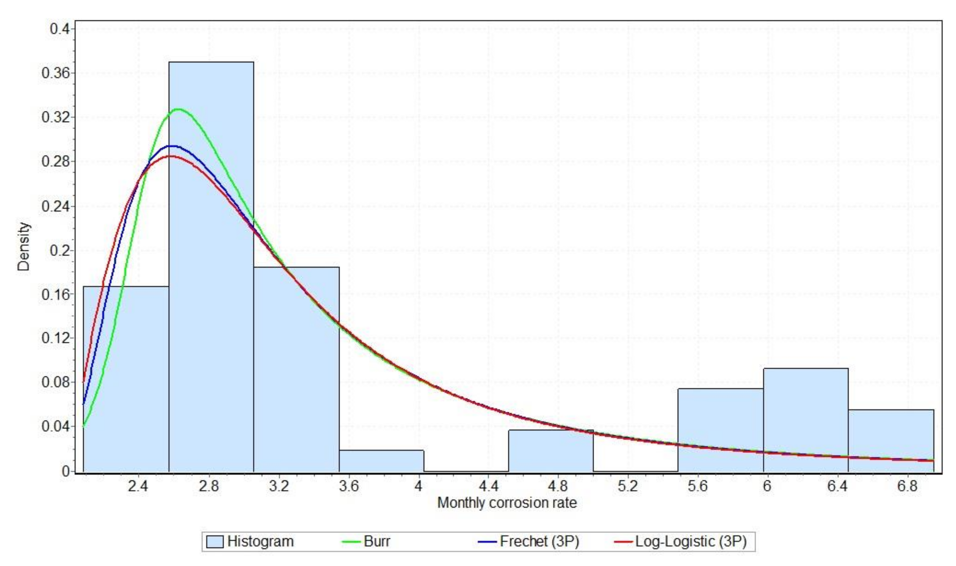
The three fitted distributions (in the case of the NiTi-1 alloy) that describe the monthly corrosion rate that occurred under the influence of air best are the shifted Log-logistic, Fréchet and Burr distributions, respectively. The expressions representing the corresponding PDFs of these distributions ($f_{a_1}^{\left(l\right)}\left(x\right)$, $f_{a_1}^{\left(f\right)}\left(x\right)$, $f_{a_1}^{\left(b\right)}\left(x\right)$) are given in Equations (11)–(13), while the expressions for the CDF ($F_{a_1}^{\left(l\right)}\left(x\right)$, $F_{a_1}^{\left(f\right)}\left(x\right)$, $F_{a_1}^{\left(b\right)}\left(x\right)$) of these distributions are shown in Equations (14)–(16).

$$f_{a_1}^{\left(l\right)}\left(x\right)=\frac{1+62206{\left(x-2.0076\right)}^{0.879}}{{\left(1+0.863256{\left(x-2.0076\right)}^{1.879}\right)}^2},x\ge 2.0076,$$

(11)

$$f_{a_1}^{\left(f\right)}\left(x\right)=\frac{1.06996e^{-\frac{1.25655}{{\left(x-1.8696\right)}^{0.85151}}}}{{\left(x-1.8696\right)}^{1.85151}},x>1.8696,$$

(12)

$$f_{a_1}^{\left(b\right)}\left(x\right)=\frac{0.238961}{{\left(1+0.638258x^{0.15485}\right)}^{3.4178}{x}^{0.84515}},x\ge 0.$$

(13)

$$F_{a_1}^{\left(l\right)}\left(x\right)=\frac{1}{1+1.1584{\left(\frac{1}{x-2.0076}\right)}^{1.879}},x\ge 2.0076,$$

(14)

$$F_{a_1}^{\left(f\right)}\left(x\right)=e^{-\frac{1.25655}{{\left(x-1.8696\right)}^{0.85151}}},x>1.8696,$$

(15)

$$F_{a_1}^{\left(b\right)}\left(x\right)=1-\frac{1}{{\left(1+0.638258x^{0.15485}\right)}^{2.4178}},x>0.$$

(16)

Mean values can be calculated for the previously determined Log-logistic, Fréchet and Burr distributions, and they are equal to 3.8249 nm/month, 3.7878 nm/month and 3.7208 nm/month, respectively. It is noticeable that these values are very close to the mean value for the corrosion rate determination in Equation (2). As this Log-Logistic distribution is a shifted standard Log-Logistic distribution, its variance, as well as the Standard Deviation cannot be calculated based on the set of these particular parameters, because, according to the formula for variance, the obtained value takes a negative value. However, the Standard Deviations for the Fréchet and Burr distributions can be calculated, and they are equal to 5.1893 nm/month and 2.4959 nm/month, respectively.

Generally speaking, if the procedure of fitting theoretical distributions is carried out correctly, the mean values of the fitted distributions always take values that are close to the mean value of the parameter $c_1$.

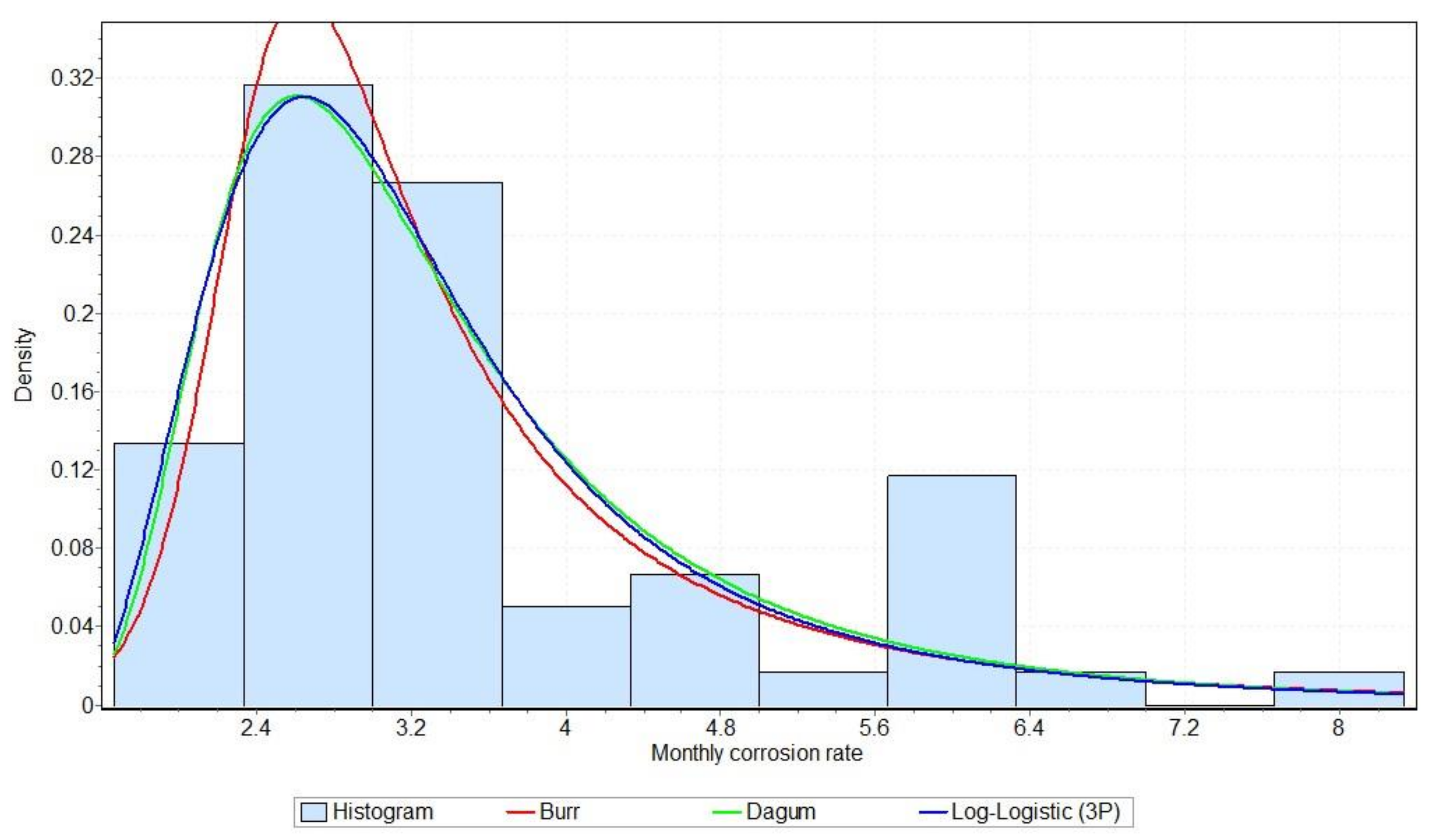
Influenced by the tide, the Burr, shifted Log-Logistic, and Dagum distributions have proven to be the three best-fitted tree parameter distributions to describe monthly corrosion rate behaviour. The terms describing their PDF ($f_{t_1}^{\left(b\right)}\left(x\right)$, $f_{t_1}^{\left(l\right)}\left(x\right)$, $f_{t_1}^{\left(d\right)}\left(x\right)$) and CDF ($F_{t_1}^{\left(b\right)}\left(x\right)$, $F_{t_1}^{\left(l\right)}\left(x\right)$, $F_{t_1}^{\left(d\right)}\left(x\right)$) are given in Equations (17)–(22), respectively.

$$f_{t_1}^{\left(b\right)}\left(x\right)=\frac{0.354244}{{\left(1+0.52122x^{0.28059}\right)}^{3.4222}{x}^{0.71941}},x>0,$$

(17)

$$f_{t_1}^{\left(l\right)}\left(x\right)=\frac{0.7836231442446434{\left(x-1.5086\right)}^{1.5145}}{{\left(1+0.3116417356311964{\left(x-1.5086\right)}^{2.5145}\right)}^2},x\ge 1.5086,$$

(18)

$$f_{t_1}^{\left(d\right)}\left(x\right)=\frac{0.09246162125573458x^{99.405731}}{{\left(1+0.7845614589000012x^{3.4851}\right)}^{29.81}},x\ge 0.$$

(19)

$$F_{t_1}^{\left(b\right)}\left(x\right)=1-\frac{1}{{\left(1+0.52122x^{0.28059}\right)}^{2.4222}},x>0$$

(20)

$$F_{t_1}^{\left(l\right)}\left(x\right)=\frac{1}{1+3.20881{\left(\frac{1}{x-1.5086}\right)}^{2.5145}},x\ge 1.5086,$$

(21)

$$F_{t_1}^{\left(d\right)}\left(x\right)=\frac{1}{{\left(1+\frac{1.274597405539211}{x^{3.4851}}\right)}^{28.81}},x\ge 0.$$

(22)

In the case of the influence of the tide on the corrosion rate of the NiTi-1 alloy, for the previously defined Burr, shifted Log-Logistic, and Dagum distributions, mean values equal to 3.6334 nm/month, 3.6023 nm/month and 3.5806 nm/month, respectively, were determined, while the Standard Deviations were 2.419 nm/month, 2.4808 nm/month and 1.8852 nm/month, respectively. It is noticeable that all mean values were very close to the mean value for the corrosion rate obtained in Equation (3).

Taking into account the probability estimates given by Equation (10) and the PDF of the best fitted Burr distribution in the case of tide influence, it was possible to calculate probabilities for corrosion wear as follows:

$$P\left(c_{a}t\le d\left(t\right)\le c_{b}t\right)={{\displaystyle \int }}_{c_a}^{c_b}\frac{0.354244}{{\left(1+0.52122x^{0.28059}\right)}^{3.4222}{x}^{0.71941}}dx,$$

(23)

where $t>0$ (months) is the elapsed time of the tide’s influence on the NiTi-1 alloy, and $0<c_a<c_b$. If values $c_a=0$, $c_b=4$ nm/month, and $t=6,12,18$ months are replaced into Equation (17), the following estimates can be calculated for probabilities:

$$\begin{array}{cc}\hfill P\left(d\left(6\right)\le 24\mathrm{nm}\right)& =P\left(d\left(12\right)\le 48\mathrm{nm}\right)=P\left(d\left(18\right)\le 72\mathrm{nm}\right)\hfill \\ & =\underset{0}{\overset{4}{{\displaystyle \int }}}\frac{0.354244}{{\left(1+0.52122x^{0.28059}\right)}^{3.4222}{x}^{0.71941}}dx=0.76236.\hfill \end{array}$$

(24)

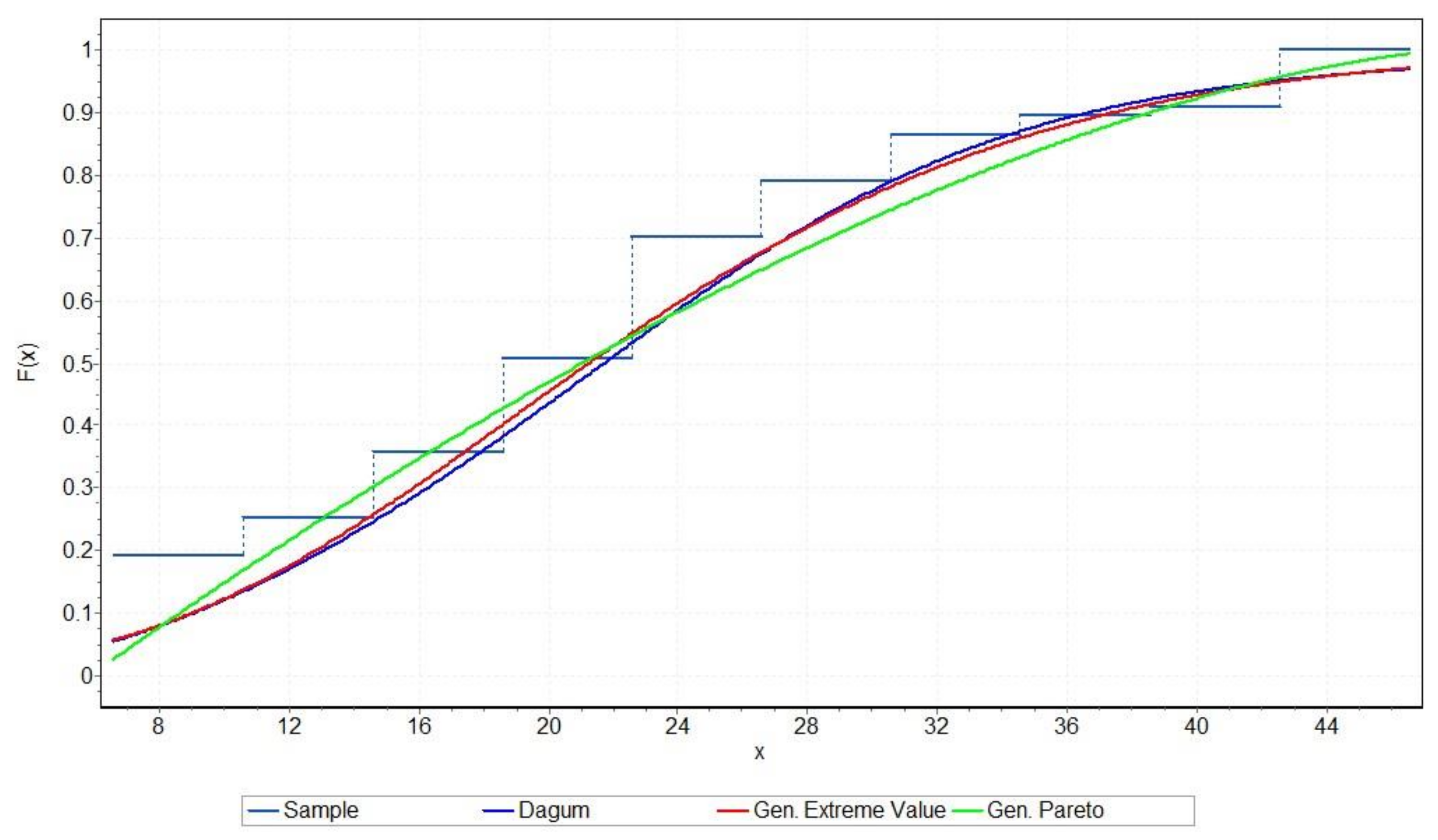
The generalised extreme value (GEV), Dagum and Generalized Pareto distributions describe the changes in the monthly corrosion rate caused by the sea best in the case of the NiTi-1 alloy. The corresponding PDF ($f_{s_1}^{\left(g\right)}\left(x\right)$, $f_{s_1}^{\left(d\right)}\left(x\right)$, $f_{s_1}^{\left(gp\right)}\left(x\right)$) and CDF ($F_{s_1}^{\left(g\right)}\left(x\right)$, $F_{s_1}^{\left(d\right)}\left(x\right)$, $F_{s_1}^{\left(gp\right)}\left(x\right)$) expressions are shown in Equations (25)–(30), respectively.

$$f_{s_1}^{\left(g\right)}\left(x\right)=\frac{0.100774e^{-\frac{1}{{(1+1.78199(0.11404+x\left)\right)}^{0.05655515}}}}{{(1+1.78199(0.11404+x\left)\right)}^{1.05655}},x<104.698,$$

(25)

$$f_{s_1}^{\left(d\right)}\left(x\right)=\frac{1.88852\times {10}^{-7}{x}^{9.37604}}{{\left(1+0.558028x^{0.33963}\right)}^{31.551}},x\ge 0,$$

(26)

$$f_{s_1}^{\left(gp\right)}\left(x\right)=0.0369{\left(1-0.02364\left(x-5.878\right)\right)}^{0.5608},5.878\le x\le 48.17.$$

(27)

$$f_{s_1}^{\left(g\right)}\left(x\right)=e^{-\frac{1}{{(1+1.78199(0.11404+x\left)\right)}^{0.05655515}}},x<104.698,$$

(28)

$$F_{s_1}^{\left(d\right)}\left(x\right)=\frac{1}{{\left(1+\frac{1.792}{x^{0.33963}}\right)}^{30.551}},x\ge 0,$$

(29)

$$F_{s_1}^{\left(gp\right)}\left(x\right)=1-{\left(1-0.02364\left(x-5.878\right)\right)}^{1.5608},5.878\le x\le 48.17.$$

(30)

The specified GEV, Dagum and Generalised Pareto distributions defined by Equations (25)–(30) have mean values of 22.396 nm/month, 22.69 nm/month and 22.396 nm/month, respectively, while their Standard Deviations are 11.205 nm/month, 11.526 nm/month and 10.936 nm/month, respectively. Even in the case of the influence of the sea on the NiTi-1 alloy, it is noticeable that the mean values were very close to the mean value of the parameter c1 given in Equation (4).

Kolmogorov–Smirnov [56] and Anderson–Darling [57] tests are used to determine goodness-of-fit. In other words, these two tests measure how well an observed theoretical distribution fits the empirical data. Results of the goodness-of-fit for the three best-fitted three-parameter distributions related to the empirical corrosion rate in the air environment in the case of NiTi-1 alloy are shown in

Table 8. Details of the goodness-of-fit tests for the alloy NiTi-1.

Air: 1.Log-Logistic (1.879, 1.0814, 2.0076)
Kolmogorov–Smirnov test				Anderson–Darling test
Statistic p-value	0.12767 0.31491			Statistic	1.367
α	0.05	0.02	0.01	α	0.05	0.02	0.01
Critical Value	0.18144	0.20289	0.21768	Critical Value	2.5018	3.2892	3.9074
Air: 2.Fréchet (0.85151, 1.3076, 1.8696)
Kolmogorov–Smirnov test				Anderson–Darling test
Statistic p-value	0.12975 0.29694			Statistic	1.3179
α	0.05	0.02	0.01	α	0.05	0.02	0.01
Critical Value	0.18144	0.20289	0.21768	Critical Value	2.5018	3.2892	3.9074
Air: 3.Burr (0.15485, 18.168, 2.4178)
Kolmogorov–Smirnov test				Anderson–Darling test
Statistic p-value	0.13164 0.28121			Statistic	1.2547
α	0.05	0.02	0.01	α	0.05	0.02	0.01
Critical Value	0.18144	0.20289	0.21768	Critical Value	2.5018	3.2892	3.9074

.

The following null and alternative hypotheses were considered in the case of both tests:

H₀. 

Data follow the specified distribution.

H_a. 

Data do not follow the specified distribution.

The standard values 0.01, 0.02 and 0.05 were used for the significance level α. A critical value was determined for each considered α value. The null hypothesis H0 is rejected if the calculated value of the test statistic is greater than the calculated critical value for the observed value of significance level α. For the Kolmogorov–Smirnov test, the p-value is calculated based on the test statistic, and denotes the threshold value of the significance level. More precisely, the null hypothesis that the theoretical distribution follows empirical data will be accepted for all values of less than the p-value. A small p-value suggests that it is unlikely that the data came from a specified distribution.

As can be seen in Table 8, all the obtained values of KS and AD test statistics for the best-fitted distributions in the air environment for the NiTi-1 alloy were less than the critical values determined for all three selected significance levels. Additionally, the KS test statistics were lower than the p-values, indicating that H0 cannot be rejected. The remaining two considered environments (tide and sea) and the best-fitted three-parameter distributions, are shown in Table 7. Regarding these environmental influences, similar values of KS and AD test statistics were obtained. Therefore, the same conclusion can be drawn for the remaining considered environments and the best fitted three-parameter distributions, that is, H0 cannot be rejected in any of the observed cases. Due to the space savings and the length of this paper, these tables are not shown in the text.

The first three columns of

Table 9. The empirical values and the values of PDF for the three best-fitted distributions for $c_1$ concerning NiTi-1.

Air
Lower Bound	Upper Bound	Empirical PDF of${\mathit{c}}_{\mathbf{1}}$	${\mathit{f}}_{{\mathit{a}}_{\mathbf{1}}}^{\left(\mathit{l}\right)}$	${\mathit{f}}_{{\mathit{a}}_{\mathbf{1}}}^{\left(\mathit{f}\right)}$	${\mathit{f}}_{{\mathit{a}}_{\mathbf{1}}}^{\left(\mathit{b}\right)}$
2	2.5045	0.148	0.18829	0.17834	0.15185
2.5045	3.009	0.333	0.27567	0.28288	0.30930
3.009	3.5135	0.241	0.18676	0.18733	0.18950
3.5135	4.018	0.019	0.11154	0.11138	0.10980
4.018	4.5225	0.000	0.06776	0.06814	0.06780
4.5225	5.027	0.037	0.04315	0.04376	0.04420
5.027	5.5315	0.000	0.02882	0.02944	0.03009
5.5315	6.036	0.074	0.02009	0.02061	0.02122
6.036	6.5405	0.093	0.01451	0.01492	0.01541
6.5405	7.045	0.056	0.01080	0.01112	0.01147
Tide
Lower Bound	Upper Bound	Empirical PDF of${\mathit{c}}_{\mathbf{1}}$	${\mathit{f}}_{{\mathit{t}}_{\mathbf{1}}}^{\left(\mathit{b}\right)}$	${\mathit{f}}_{{\mathit{t}}_{\mathbf{1}}}^{\left(\mathit{l}\right)}$	${\mathit{f}}_{{\mathit{t}}_{\mathbf{1}}}^{\left(\mathit{d}\right)}$
1	1.743333	0.017	0.00959	0.00808	0.00776
1.743333	2.486667	0.133	0.19950	0.21955	0.21636
2.486667	3.23	0.433	0.35833	0.32213	0.31896
3.23	3.973333	0.167	0.19035	0.20092	0.19905
3.973333	4.716667	0.033	0.09372	0.10316	0.10625
4.716667	5.46	0.050	0.05078	0.05412	0.05750
5.46	6.203333	0.033	0.02989	0.03037	0.03269
6.203333	6.946667	0.117	0.01876	0.01822	0.01958
6.946667	7.69	0.000	0.01238	0.01158	0.01229
7.69	8.433333	0.017	0.00851	0.00772	0.00804
Sea
Lower Bound	Upper Bound	Empirical PDF of${\mathit{c}}_{\mathbf{1}}$	${\mathit{f}}_{{\mathit{s}}_{\mathbf{1}}}^{\left(\mathit{g}\right)}$	${\mathit{f}}_{{\mathit{s}}_{\mathbf{1}}}^{\left(\mathit{d}\right)}$	${\mathit{f}}_{{\mathit{s}}_{\mathbf{1}}}^{\left(\mathit{g}\mathit{p}\right)}$
0	4.75275	0.000	0.02808	0.02958	0.02285
4.75275	9.5055	0.179	0.07661	0.08017	0.10774
9.5055	14.25825	0.075	0.13488	0.12560	0.16092
14.25825	19.011	0.119	0.17146	0.16283	0.14874
19.011	23.76375	0.164	0.17137	0.17866	0.13570
23.76375	28.5165	0.224	0.14352	0.15896	0.12160
28.5165	33.26925	0.090	0.10540	0.11273	0.10607
33.26925	38.022	0.045	0.07004	0.06728	0.08852
38.022	42.77475	0.015	0.04293	0.03689	0.06758
42.77475	47.5275	0.090	0.02455	0.01989	0.03880

and

Table 10. The empirical values and the values of CDF for the three best-fitted distributions for $c_1$ concerning NiTi-1.

Air
Lower Bound	Upper Bound	Empirical CDF of${\mathit{c}}_{\mathbf{1}}$	${\mathit{F}}_{{\mathit{a}}_{\mathbf{1}}}^{\left(\mathit{l}\right)}$	${\mathit{F}}_{{\mathit{a}}_{\mathbf{1}}}^{\left(\mathit{f}\right)}$	${\mathit{F}}_{{\mathit{a}}_{\mathbf{1}}}^{\left(\mathit{b}\right)}$
2	2.5045	0.148	0.18829	0.17834	0.15185
2.5045	3.009	0.481	0.46397	0.46123	0.46115
3.009	3.5135	0.722	0.65073	0.64855	0.65065
3.5135	4.018	0.741	0.76227	0.75993	0.76045
4.018	4.5225	0.741	0.83003	0.82808	0.82825
4.5225	5.027	0.778	0.87318	0.87184	0.87245
5.027	5.5315	0.778	0.90201	0.90128	0.90254
5.5315	6.036	0.852	0.92209	0.92188	0.92376
6.036	6.5405	0.944	0.93660	0.93680	0.93917
6.5405	7.045	1.000	0.94741	0.94792	0.95065
Tide
Lower Bound	Upper Bound	Empirical CDF of${\mathit{c}}_{\mathbf{1}}$	${\mathit{F}}_{{\mathit{t}}_{\mathbf{1}}}^{\left(\mathit{b}\right)}$	${\mathit{F}}_{{\mathit{t}}_{\mathbf{1}}}^{\left(\mathit{l}\right)}$	${\mathit{F}}_{{\mathit{t}}_{\mathbf{1}}}^{\left(\mathit{d}\right)}$
1	1.743333	0.017	0.00959	0.00808	0.00776
1.743333	2.486667	0.150	0.20910	0.22763	0.22412
2.486667	3.23	0.583	0.56744	0.54977	0.54309
3.23	3.973333	0.750	0.75779	0.75070	0.74214
3.973333	4.716667	0.783	0.85150	0.85385	0.84838
4.716667	5.46	0.833	0.90228	0.90797	0.90588
5.46	6.203333	0.867	0.93218	0.93835	0.93857
6.203333	6.946667	0.983	0.95094	0.95657	0.95815
6.946667	7.69	0.983	0.96332	0.96815	0.97045
7.69	8.433333	1.000	0.97183	0.97587	0.97848
Sea
Lower Bound	Upper Bound	Empirical CDF of${\mathit{c}}_{\mathbf{1}}$	${\mathit{F}}_{{\mathit{s}}_{\mathbf{1}}}^{\left(\mathit{g}\right)}$	${\mathit{F}}_{{\mathit{s}}_{\mathbf{1}}}^{\left(\mathit{d}\right)}$	${\mathit{F}}_{{\mathit{s}}_{\mathbf{1}}}^{\left(\mathit{g}\mathit{p}\right)}$
0	4.75275	0.000	0.03439	0.02958	0.02285
4.75275	9.5055	0.179	0.11100	0.10975	0.13059
9.5055	14.25825	0.254	0.24588	0.23534	0.29151
14.25825	19.011	0.373	0.41733	0.39816	0.44024
19.011	23.76375	0.537	0.58871	0.57682	0.57593
23.76375	28.5165	0.761	0.73224	0.73579	0.69754
28.5165	33.26925	0.851	0.83765	0.84853	0.80362
33.26925	38.022	0.896	0.90769	0.91581	0.89213
38.022	42.77475	0.910	0.95062	0.95270	0.95972
42.77475	47.5275	1.000	0.97517	0.97259	0.99852

were obtained based on empirical data. The data range of the empirical data was divided into 10 intervals of equal width. The bounds of these intervals define the lower and upper bounds shown in the first two columns of Table 9 and Table 10. The third column of Table 9 and Table 10 were obtained based on Equation (8) and the previously described procedure for calculating empirical PDFs and CDFs. The last three columns in Table 9 for air, tide and sea environments, and for the case of the NiTi-1 alloy, were calculated based on Equations (11)–(13), (17)–(19) and (25)–(27), respectively.

The last three columns of Table 10 show the CDF values for the three best-fitted three-parameter distributions in the air, tide and sea environments for the NiTi-1 alloy. These values were calculated for each observed interval and air, tide and sea environments, according to Equations (14)–(16), (20)–(22) and (28)–(30), respectively.

Figure 11, Figure 12 and Figure 13 show the PDF and CDF graphs of the three best-fitted distributions for the air, tide and sea environments in the case of the NiTi-1 alloy, respectively. These graphs also contain a representation of the empirical PDF or the empirical CDF accordingly. These figures correspond to the numerical results given in Table 9 and Table 10.

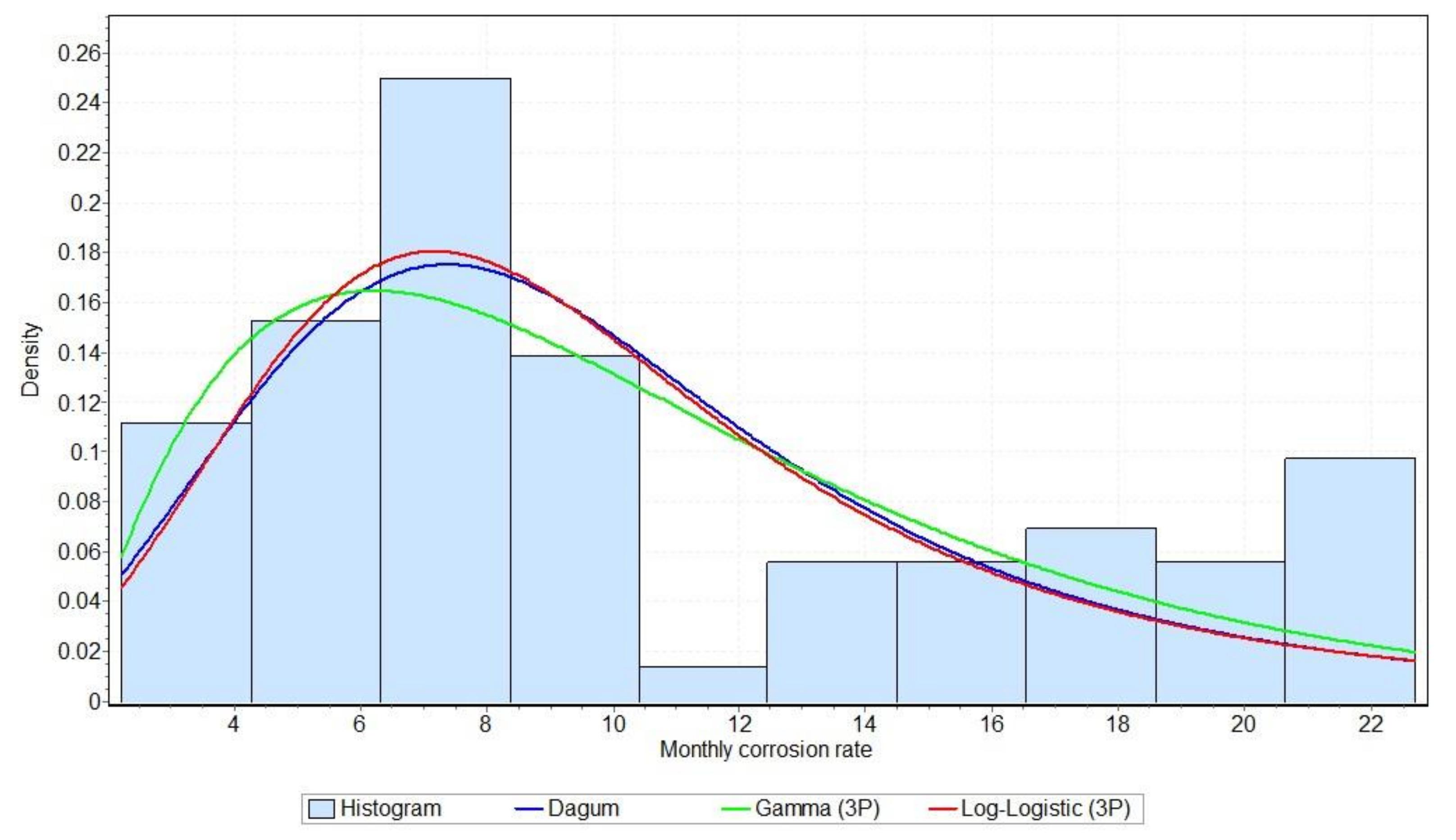
The similarity of empirical data related to air and tide influence on the NiTi-1 alloy can be observed in Figure 11 and Figure 12. The histograms of these two datasets have almost the same shape. It can be seen that the empirical data for the corrosion rate in the case of the NiTi-1 alloy and the influence of air and tide are unimodal, and show highly skewed tendencies with heavy right tails. Additionally, these two figures show that all fitted three-parameter distributions follow the shape of the corrosion empirical data in the air and tide environments.

The corrosion rate that occurred under the influence of air on NiTi-1 had initially increasing values, while later it decreased, so the three-parameter Log-logistic distribution proved to be the most favourable theoretical distribution. Considering that the Burr distribution is a generalisation of the Log-Logistics distribution, it becomes clear why they follow this empirical data best in the case of the NiTi-1 alloy under air influence.

The Burr distribution is a flexible distribution that adapts easily and well to complex changes in empirical data, especially from the point of view of skewness and kurtosis. Burr distribution is very suitable to model the skewness of distribution, and, at the same time, tail behaviour. Empirical data related to the NiTi-1 alloy corrosion rate influenced by the tide show a high peak and long thin right tail. Therefore, Burr distribution can be used to model these extremes of empirical data well.

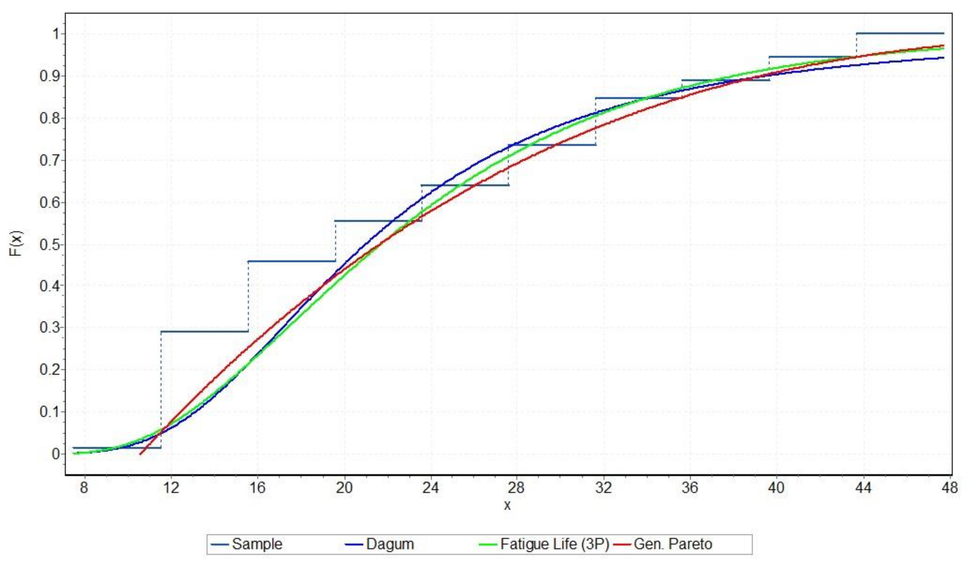
The results of fitting the theoretical distributions into the empirical data related to the influence of the sea on the NiTi-1 alloy are shown visually in Figure 13 as empirical CDF and best-fitted CDFs. These figures show clearly the similarity of the shapes of all three theoretical CDFs, and, at the same time, these three best CDFs follow the empirical data adequately. Empirical data related to the influence of the sea are bimodal and approximately symmetric, in contrast to the empirical data on the corrosion rate concerning the influence of air and tide. As a result, distributions with slightly different characteristics from those previously selected for air and tide proved to be the best theoretical distributions in the case of the sea’s influence on the NiTi-1 alloy. Similar graphs can be produced for the influence of air and tide on the corrosion rate in the case of the NiTi-1 alloy.

GEV is a kind of distribution that can model the distribution of extreme maximum values suitably. Extreme corrosion rate values can have a significant impact, especially when considering the use of an alloy in everyday real-life conditions. The importance of timely prevention of the harmful effects of corrosion on the exploitation of the alloy, as well as the fact that the GEV distribution proved to be a suitable model for describing the corrosion rate in the conditions of the dominant influence of the sea, indicates that it is worth investigating the extreme value theory [58] concerning the NiTi-1 alloy empirical data, especially in the case of the sea environment’s influence.

The probability-probability plot (P-P plot) shown in Figure 14 was used to compare the goodness of fit of the three best-fitted theoretical distributions related to the empirical data obtained for the influence of the sea on the corrosion processes of the NiTi-1 alloy visually [59]. This figure was used to visualise the plots of the three best-fitting CDFs shown against the empirical CDFs, which was used as the reference distribution. In this way, it was possible to compare the empirical CDFs visually with the corresponding theoretical CDFs. Figure 14 shows the linearity of the plotted data, i.e., that the points are approximately distributed along the diagonals of the graphs. This linearity indicates an adequately implemented procedure for fitting three-parameter distributions into empirical data.

Slight deviations from linearity can be observed in the tails of the distributions. This phenomenon of deviation from the linear trend in the tails is not surprising, given that the empirical data are right-skewed. Due to this type of data scattering, it often happens that tail regions have noisy effects on the model characteristics, and thus can affect the performance of the statistical model negatively. Similar graphs were obtained for the influence of air and tide on the corrosion processes of the NiTi-1 alloy.

3.2. Results of Statistical Analysis for the NiTi-2 Alloy

The previously used set of 27 theoretical continuous distributions was additionally fitted into the empirical data relating to the monthly corrosion rate in the NiTi-2 alloys. All fitted results were validated using KS and AD tests, and ranked based on the test statistics obtained over the KS test. In this way, the three best-fitted distributions were selected for the air, tide and water environments in the case of the NiTi-2 alloy. The three best-fitted distributions with the best-performing parameters are shown in

Table 11. The three best-fitted three-parameter distributions for the NiTi-2 alloy in air, tide and sea environments.

Environment	Distribution (Parameters)	KS Ranking	AD Ranking
Air	Burr (0.15416, 21.51, 2.715)	1	1
	Log-Logistic (2.2589, 1.1902, 2.1909)	2	3
	Fréchet (0.68413, 1.4445, 2.0152)	3	2
Tide	Log-Logistic (2.9765, 9.4705, −0.31248)	1	1
	Dagum (0.80238, 3.1011, 10.229)	2	2
	Gamma (2.0829, 4.4208, 1.43)	3	3
Sea	General Pareto (−0.33758, 17.894, 10.585)	1	20
	Dagum (3.16, 3.1334, 13.409)	2	8
	Fatigue Life (0.48433, 19.344, 2.3488)	3	2

for each observed seawater environment.

The expressions in Equations (31)–(33) were formed for the three best-fitted three-parameter distributions detected for the air environment, using standard expressions describing the corresponding PDFs and substituting the calculated values of all three parameters. These formulas represent analytical forms of PDFs related to the Burr, Log-Logistic and Fréchet distributions.

$$f_{a_2}^{\left(b\right)}\left(x\right)=\frac{0.260796}{{\left(1+0.623103x^{0.15416}\right)}^{3.715}{x}^{0.84584}},x\ge 0$$

(31)

$$f_{a_2}^{\left(l\right)}\left(x\right)=\frac{1.52433{\left(x-2.1909\right)}^{1.2589}}{{\left(1+0.674811{\left(x-2.1909\right)}^{2.2589}\right)}^2},x\ge 2.1909,$$

(32)

$$f_{a_2}^{\left(f\right)}\left(x\right)=\frac{0.879845e^{-\frac{1.286078}{{\left(x-2.0152\right)}^{0.68413}}}}{{\left(x-2.0152\right)}^{1.68413}},x>2.0152.$$

(33)

Based on the previously determined set of three parameters for each of the observed theoretical distributions for the air environment (Table 11), taking into account their PDF Equations (31)–(33), adequate CDF formulas for the best fitted Burr, Log-Logistic and Fréchet distributions for the air environment were determined, as is shown in Equations (34)–(36).

$$F_{a_2}^{\left(b\right)}\left(x\right)=1-\frac{1}{{\left(1+0.623103x^{0.15416}\right)}^{2.715}},x\ge 0$$

(34)

$$F_{a_2}^{\left(l\right)}\left(x\right)=\frac{1}{1+1.4819{\left(\frac{1}{x-2.1909}\right)}^{2.2589}},x\ge 2.1909,$$

(35)

$$F_{a_2}^{\left(f\right)}\left(x\right)=e^{-\frac{1.286078}{{\left(x-2.0152\right)}^{0.68413}}},x>2.0152.$$

(36)

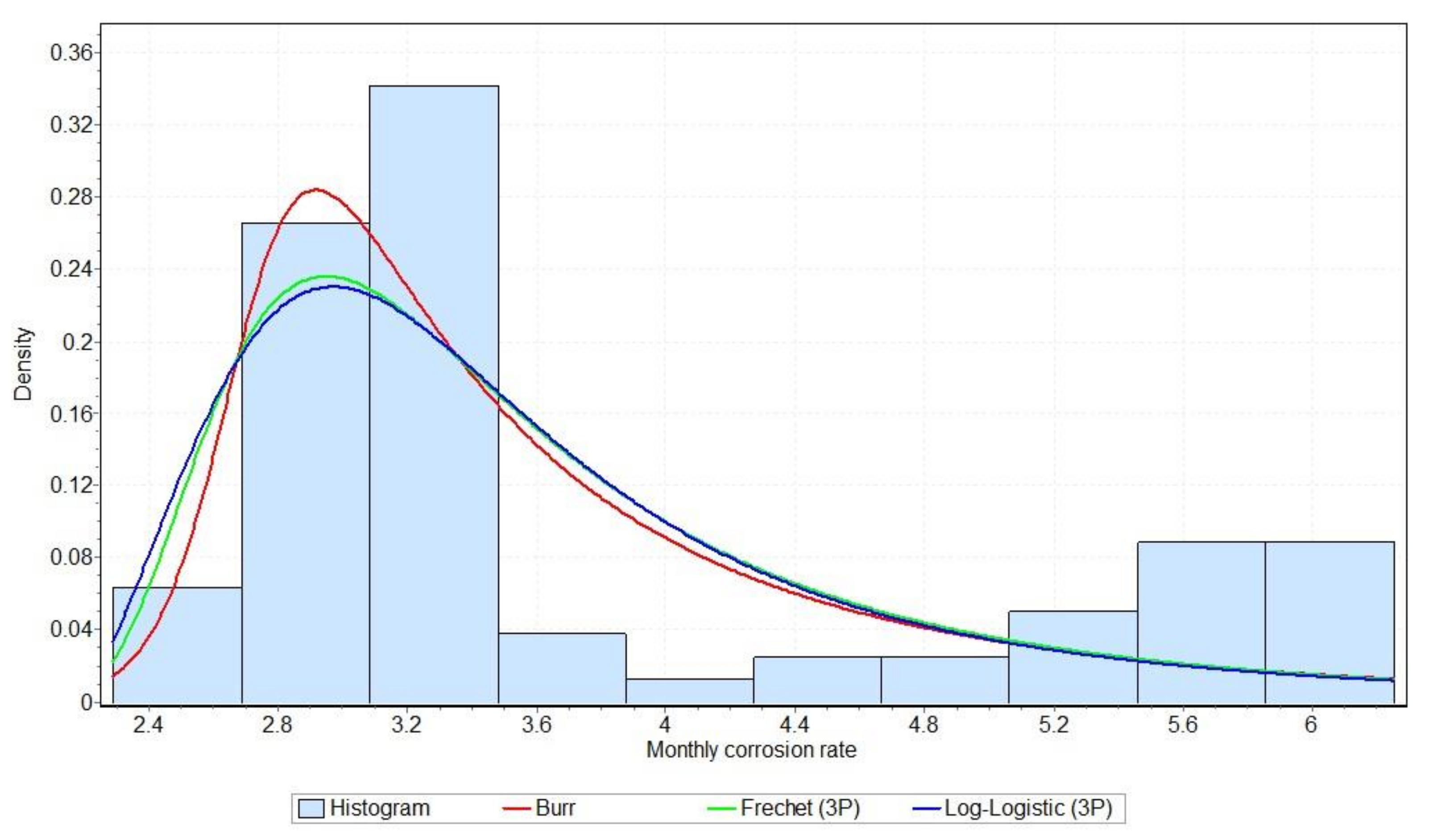
The mean values of the previously specified Burr, Log-Logistic, and Fréchet distributions (3.8585 nm/month, 3.8734 nm/month, 3.8519 nm/month, respectively, with Standard Deviations of 1.8785 nm/month, 2.89 nm/month, 1.9212 nm/month, respectively), were taking values very close to the calculated mean value of the parameter $c_1$ from Equation (5), showing the correctness of the distribution fitting approach.

By applying the statistical procedure of fitting three-parameter distributions, the Log-Logistic, Dagum and Gamma distributions proved to be the three best theoretical distributions for describing empirical data of the corrosion rate caused by the tide’s influence. After incorporating the best values of the three parameters, the PDFs of these three functions yielded in Equations (37)–(39).

$$f_{t_2}^{\left(l\right)}\left(x\right)=\frac{0.0036943{\left(0.31248+x\right)}^{1.9765}}{{\left(1+0.00124116{\left(0.31248-x\right)}^{2.9765}\right)}^2},x\ge -0.31248,$$

(37)

$$f_{t_2}^{\left(d\right)}\left(x\right)=\frac{0.00764131x^{1.488260618}}{{\left(1+0.000738595x^{3.1011}\right)}^{1.80238}},x\ge 0,$$

(38)

$$f_{t_2}^{\left(g\right)}\left(x\right)=0.0435831{\mathrm{e}}^{-0.226203\left(x-1.43\right)}{\left(x-1.43\right)}^{1.0829},x\ge 1.43.$$

(39)

The Log-Logistic, Dagum and Gamma distributions prove to be the best fitted three-parameter distributions for the tidal environment. The corresponding CDF formulas, specified by the set of the best parameter values, are shown in Equations (40)–(42).

$$F_{t_2}^{\left(l\right)}\left(x\right)=\frac{1}{1+805.701{\left(\frac{1}{0.31248+x}\right)}^{2.9765}},x\ge -0.31248,$$

(40)

$$F_{t_2}^{\left(d\right)}\left(x\right)=\frac{1}{{\left(1+\frac{1353.92}{x^{3.1011}}\right)}^{0.80238}},x\ge 0,$$

(41)

$$F_{t_2}^{\left(g\right)}\left(x\right)=0.9635\left(1.03793-\underset{0.226203\left(x-1.43\right)}{\overset{\infty }{{\displaystyle \int }}}{t}^{1.0829}{e}^{-t}dt\right),x\ge 1.43.$$

(42)

For the three best-fitted three-parameter distributions in the case of NiTi-2 alloy and tidal environment, it can be shown that their mean values had approximately the same value as the mean corrosion rate from Equation (6). Namely, the mean values were 11.175 nm/month, 11.072 nm/month and 10.638 nm/month, respectively, while the Standard Deviations were, respectively, 9.4225 nm/month, 8.8037 nm/month and 6.3802 nm/month.

PDFs and CDFs of the best fitted three-parameter distributions (Generalised Pareto, Dagum and Fatigue Life) in the case of the sea environment are shown in Equations (43)–(48), respectively. Note that, as in the previous expressions, we substituted into general expressions for distributions PDF and CDF the values of the best-fitting parameters.

$$f_{s_2}^{\left(gp\right)}\left(x\right)=0.0559{\left(1-0.0189\left(x-10.585\right)\right)}^{1.96226},10.585\le x\le 63.59,$$

(43)

$$f_{s_2}^{\left(d\right)}\left(x\right)=\frac{6.80359\ast {10}^{-11}{x}^{8.901544}}{{\left(1+0.00029337x^{3.1334}\right)}^{4.16}},x\ge 0,$$

(44)

$$\begin{gathered} f_{s_2}^{\left(fl\right)}\left(x\right)=e^{-2.13{\left(4.398\sqrt{\frac{1}{x-2.3488}}-0.227\sqrt{x-2.3488}\right)}^2}\ast \\ \frac{0.41\left(4.398\sqrt{\frac{1}{x-2.3488}}+0.227\sqrt{x-2.3488}\right)}{x-2.3488},x>2.3488. \end{gathered}$$

(45)

$$F_{s_2}^{\left(gp\right)}\left(x\right)=1-{\left(1-0.0189\left(x-10.585\right)\right)}^{2.96226},10.585\le x\le 63.59,$$

(46)

$$F_{s_2}^{\left(d\right)}\left(x\right)=\frac{1}{{\left(1+\frac{3408.66}{x^{3.1334}}\right)}^{3.16}},x\ge 0,$$

(47)

$$F_{s_2}^{\left(fl\right)}\left(x\right)=\mathsf{\Phi }\left[2.065\left(-4.4\sqrt{\frac{1}{x-2.3488}}+0.23\sqrt{x-2.3488}\right)\right],x>2.3488,$$

(48)

where $\mathsf{\Phi }\left[x\right]$ represents the Laplace integral, i.e., $\mathsf{\Phi }\left[x\right]=\frac{1}{\sqrt{2\pi }}{{\displaystyle \int }}_0^x{e}^{-\frac{t^2}{2}dt}$.

The mean value of corrosion rate from Equation (7) has a very close value to all three mean values of the specified Generalised Pareto, Dagum and Fatigue Life distributions. These mean values were 23.963 nm/month, 24.853 nm/month and 23.962 nm/month, respectively, while the Standard Deviations were, 10.336 nm/month, 16.491 nm/month and 10.655 nm/month, respectively, proving the fact that these three distributions are describing well the empirical data related to the sea environment and the NiTi-2 alloy.

As an example, probability estimates for related corrosion wear due to the influence of the sea environment concerning the NiTi-2 alloy can be calculated based on the best fitted Generalised Pareto PDF Equation (43) and the estimate given by Equation (10), as follows:

$$P\left(c_{a}t\le d\left(t\right)\le c_{b}t\right)={{\displaystyle \int }}_{c_a}^{c_b}0.0559{\left(1-0.0189\left(x-10.585\right)\right)}^{1.96226}dx,$$

(49)

where $t>0$ (months) is the elapsed time of the sea’s influence on the NiTi-2 alloy, and $10.585\le c_a<c_b\le 63.59$. For example, if $c_a=11$ nm/month, $c_b=13$ nm/month, and $t=6,12,18$ months are taken, and these values are replaced into Equation (49), the following estimates can be calculated for probabilities:

$$\begin{array}{cc}P\left(66\mathrm{nm}\le d\left(6\right)\le 78\mathrm{nm}\right)& =P\left(132\mathrm{nm}\le d\left(12\right)\le 156\mathrm{nm}\right)\hfill \\ & =P\left(198\mathrm{nm}\le d\left(18\right)\le 234\mathrm{nm}\right)\hfill \\ & =\underset{11}{\overset{13}{{\displaystyle \int }}}0.0559{\left(1-0.0189\left(x-10.585\right)\right)}^{1.96226}dx=0.106.\hfill \end{array}$$

(50)

In the case of the NiTi-2 alloy we used the same approach as in the case of the NiTi-1 alloy, to address the goodness-of-fit. Namely, Kolmogorov–Smirnov and Anderson–Darling tests were used to determine the three best fitted theoretical distributions which can describe monthly corrosion rate adequately in each observed seawater environment. The results of these tests for the air environment are shown in

Table 12. Details of the goodness-of-fit tests for the alloy NiTi-2.

Air: 1. Burr (0.15416, 21.51, 2.715)
Kolmogorov–Smirnov test				Anderson–Darling test
Statistic p-value	0.11397 0.23764			Statistic	1.5013
α	0.05	0.02	0.01	α	0.05	0.02	0.01
Critical Value	0.15052	0.16832	0.1806	Critical Value	2.5018	3.2892	3.9074
Air: 2. Log-Logistic (2.2589, 1.1902, 2.1909)
Kolmogorov–Smirnov test				Anderson–Darling test
Statistic p-value	0.1292 10.13081			Statistic	1.9414
α	0.05	0.02	0.01	α	0.05	0.02	0.01
Critical Value	0.15052	0.16832	0.1806	Critical Value	2.5018	3.2892	3.9074
Air: 3. Frechet (0.68413, 1.4445, 2.0152)
Kolmogorov–Smirnov test				Anderson–Darling test
Statistic p-value	0.13424 0.10566			Statistic	1.8828
α	0.05	0.02	0.01	α	0.05	0.02	0.01
Critical Value	0.15052	0.16832	0.1806	Critical Value	2.5018	3.2892	3.9074

.

Table 12 has the same structure as Table 8, and it shows details of the goodness-of-fit tests for the NiTi-2 alloy in the air environment. KS and AD tests were employed to check the goodness-of-fit of the selected best-fitted three-parameter theoretical distributions for all observed seawater environments in the case of the NiTi-2 alloy. The results related to these tests in the case of the air environment are presented in Table 12. Both statistical tests were performed with the same values of significance level ($\alpha =0.05,0.02,$ and $0.01$). Adequate critical values were calculated for each test and each significance level, with the addition of p-values for the KS test. Moreover, the same hypotheses, H0 and Ha, were set up as in the case of the NiTi-1 alloy.

Based on the obtained values of the test statistics, it can be concluded that hypothesis H0 cannot be rejected in any of the tested cases, because the test statistics for all calculations were less than the corresponding critical values for the considered significance levels. Moreover, the test statistics for the KS test were less than the calculated p-values, which is another indicator that the considered fitted distributions follow the empirical data well, i.e., that the null hypothesis cannot be rejected. For the remaining best fitted three-parameter distributions (see Table 11) very similar hypothesis testing results were obtained, meaning that, in the case of tidal and sea effects on the corrosion processes of the NiTi-2 alloy, the null hypothesis also cannot be rejected. These hypotheses testing results were omitted from the text because a lot of space is necessary for their presentation.

Table 13. The empirical values and the values of PDF for the three best-fitted distributions for $c_1$ concerning NiTi-2.

Air
Lower Bound	Upper Bound	Empirical PDF of${\mathit{c}}_{\mathbf{1}}$	${\mathit{f}}_{{\mathit{a}}_{\mathbf{2}}}^{\left(\mathit{b}\right)}$	${\mathit{f}}_{{\mathit{a}}_{\mathbf{2}}}^{\left(\mathit{l}\right)}$	${\mathit{f}}_{{\mathit{a}}_{\mathbf{2}}}^{\left(\mathit{f}\right)}$
2	2.435	0.025	0.01385	0.02715	0.02134
2.435	2.87	0.190	0.18738	0.19253	0.19026
2.87	3.305	0.329	0.27879	0.24306	0.24657
3.305	3.74	0.165	0.17412	0.18184	0.18053
3.74	4.175	0.013	0.10563	0.11573	0.11574
4.175	4.61	0.013	0.06723	0.07201	0.07337
4.61	5.045	0.038	0.04466	0.04590	0.04758
5.045	5.48	0.051	0.03073	0.03034	0.03182
5.48	5.915	0.089	0.02179	0.02079	0.02195
5.915	6.35	0.089	0.01585	0.01473	0.01557
Tide
Lower Bound	Upper Bound	Empirical PDF of${\mathit{c}}_{\mathbf{1}}$	${\mathit{f}}_{{\mathit{t}}_{\mathbf{2}}}^{\left(\mathit{l}\right)}$	${\mathit{f}}_{{\mathit{t}}_{\mathbf{2}}}^{\left(\mathit{d}\right)}$	${\mathit{f}}_{{\mathit{t}}_{\mathbf{2}}}^{\left(\mathit{g}\right)}$
0	2.3685	0.028	0.02283	0.02602	0.01590
2.3685	4.737	0.097	0.11048	0.11122	0.13891
4.737	7.1055	0.222	0.19252	0.18541	0.18772
7.1055	9.474	0.264	0.19857	0.19567	0.17524
9.474	11.8425	0.056	0.15321	0.15575	0.14199
11.8425	14.211	0.028	0.10362	0.10700	0.10670
14.211	16.5795	0.083	0.06723	0.06945	0.07647
16.5795	18.948	0.069	0.04373	0.04480	0.05310
18.948	21.3165	0.083	0.02900	0.02935	0.03601
21.3165	23.685	0.069	0.01973	0.01969	0.02399
Sea
Lower Bound	Upper Bound	Empirical PDF of${\mathit{c}}_{\mathbf{1}}$	${\mathit{f}}_{{\mathit{s}}_{\mathbf{2}}}^{\left(\mathit{g}\mathit{p}\right)}$	${\mathit{f}}_{{\mathit{s}}_{\mathbf{2}}}^{\left(\mathit{d}\right)}$	${\mathit{f}}_{{\mathit{s}}_{\mathbf{2}}}^{\left(\mathit{f}\mathit{l}\right)}$
0	4.8685	0.000	0	0.00004	0.00011
4.8685	9.737	0.014	0.00026	0.01563	0.01936
9.737	14.6055	0.194	0.20807	0.15039	0.15149
14.6055	19.474	0.250	0.21117	0.25947	0.22978
19.474	24.3425	0.139	0.16989	0.20983	0.20386
24.3425	29.211	0.097	0.33230	0.13252	0.14745
29.211	34.0795	0.139	0.10092	0.07957	0.09698
34.0795	38.948	0.042	0.07300	0.04848	0.06067
38.948	43.8165	0.083	0.04955	0.03054	0.03690
43.8165	48.685	0.042	0.03057	0.01994	0.02206

shows the numerical results for the empirical PDFs and the three best-fitted theoretical PDFs for the corrosion rate in the case of the NiTi-2 alloy and the influence of the air, tide and sea on corrosion processes. Empirical data were sorted into bins obtained by dividing the data range into ten equal intervals. Interval limits were defined by their lower and upper bounds. After arranging the empirical data into bins and calculating the empirical PDFs adequately in the process of fitting the three-parameter distributions, the numerical values for the theoretical PDFs shown in the last three columns of Table 13 were determined by employing Equations (31)–(33) in the case of air influence, Equations (37)–(39) in the case of tidal influence and Equations (43)–(45) in the case of the sea’s influence on the NiTi-2 alloy.

Figure 15 and Figure 16 show the empirical PDFs and best-fitted theoretical PDFs for the NiTi-2 alloy in air and tidal environments, respectively. It can be seen from the figures that the fitted distributions followed the empirical data well in both cases. The empirical data are unimodal, moderately right skewed, with a notable tail, especially in the case of exposing the alloy to an air influence. A similar graph can be formed for the influence of the sea on the corrosion rate in the case of the NiTi-2 alloy.

From Figure 15 and Figure 16 it is notable that the best-fitted theoretical distributions are positively skewed, i.e., skewed to the right. Based on this, it was concluded that a small number of corrosion rates would have high values. As a result, it was not surprising that the Log-Logistic and Burr distributions proved to be the most favourable, because they had the property of following the empirical data well, by which the most frequent events occurred at the beginning of the observed intervals.

The lower and upper bounds of the intervals in

Table 14. The empirical values and the values of CDF for the three best-fitted distributions for $c_1$ concerning NiTi-2.

Air
Lower Bound	Upper Bound	Empirical CDF of${\mathit{c}}_{\mathbf{1}}$	${\mathit{F}}_{{\mathit{a}}_{\mathbf{2}}}^{\left(\mathit{b}\right)}$	${\mathit{F}}_{{\mathit{a}}_{\mathbf{2}}}^{\left(\mathit{l}\right)}$	${\mathit{F}}_{{\mathit{a}}_{\mathbf{2}}}^{\left(\mathit{f}\right)}$
2	2.435	0.025	0.01407	0.02715	0.02143
2.435	2.87	0.215	0.20144	0.21968	0.21159
2.87	3.305	0.544	0.48023	0.46274	0.45816
3.305	3.74	0.709	0.65435	0.64458	0.63869
3.74	4.175	0.722	0.75999	0.76030	0.75444
4.175	4.61	0.734	0.82722	0.83232	0.82781
4.61	5.045	0.772	0.87187	0.87822	0.87539
5.045	5.48	0.823	0.90261	0.90855	0.90721
5.48	5.915	0.911	0.92440	0.92935	0.92916
5.915	6.35	1.000	0.94025	0.94408	0.94473
Tide
Lower Bound	Upper Bound	Empirical CDF of${\mathit{c}}_{\mathbf{1}}$	${\mathit{F}}_{{\mathit{t}}_{\mathbf{2}}}^{\left(\mathit{l}\right)}$	${\mathit{F}}_{{\mathit{t}}_{\mathbf{2}}}^{\left(\mathit{d}\right)}$	${\mathit{F}}_{{\mathit{t}}_{\mathbf{2}}}^{\left(\mathit{g}\right)}$
0	2.3685	0.028	0.02283	0.02602	0.01590
2.3685	4.737	0.125	0.13332	0.13725	0.15482
4.737	7.1055	0.347	0.32584	0.32266	0.34254
7.1055	9.474	0.611	0.52441	0.51832	0.57780
9.474	11.8425	0.667	0.67761	0.67407	0.65977
11.8425	14.211	0.694	0.78121	0.78105	0.76645
14.211	16.5795	0.778	0.84844	0.85050	0.84292
16.5795	18.948	0.847	0.89216	0.89529	0.89601
18.948	21.3165	0.931	0.92116	0.92464	0.93202
21.3165	23.685	1.000	0.94089	0.94434	0.95601
Sea
Lower Bound	Upper Bound	Empirical CDF of${\mathit{c}}_{\mathbf{1}}$	${\mathit{F}}_{{\mathit{s}}_{\mathbf{2}}}^{\left(\mathit{g}\mathit{p}\right)}$	${\mathit{F}}_{{\mathit{s}}_{\mathbf{2}}}^{\left(\mathit{d}\right)}$	${\mathit{F}}_{{\mathit{s}}_{\mathbf{2}}}^{\left(\mathit{f}\mathit{l}\right)}$
0	4.8685	0.000	0	0.00004	0.00011
4.8685	9.737	0.014	0.00026	0.01567	0.01947
9.737	14.6055	0.208	0.20833	0.16606	0.17096
14.6055	19.474	0.458	0.41949	0.42550	0.40071
19.474	24.3425	0.597	0.58938	0.63533	0.60457
24.3425	29.211	0.694	0.72263	0.76786	0.75204
29.211	34.0795	0.833	0.82355	0.84743	0.84902
34.0795	38.948	0.875	0.89656	0.89591	0.90970
38.948	43.8165	0.958	0.94611	0.92644	0.94660
43.8165	48.685	1.000	0.97667	0.94639	0.96566

are the same as in Table 13, and were obtained by binning of the empirical data in ten equal-width intervals. Numerical results for the empirical CDFs were calculated based on the previously obtained empirical PDFs, while for calculation of the numerical results of the three best fitted theoretical three-parameter CDFs, the previously presented formulas were used, namely, Equations (34)–(36) for CDF functions describing the influence of air on the NiTi-2 alloy, Equations (40)–(42) for tidal influence and Equations (46)–(48) for the sea’s influence.

The numerical data from the last part of Table 14, which refer to the influence of the sea environment on the corrosion rate of NiTi-2 alloy, are presented graphically in Figure 17. The empirical CDF is shown by a step function. It is noticeable that all three of the best-fitted theoretical distributions followed the form of the empirical CDF adequately, and can be considered as a good approximation of these empirical data.

In the case of the sea environment’s influence on NiTi-2 alloys, the empirical data of corrosion rate show heavy tail tendencies. The Generalised Pareto distribution can model this kind of empirical data well, because this type of distribution produces extreme events, with the tendency that its density reduces value polynomially. This characteristic of the Generalised Pareto distribution justifies the reason why it was chosen as the best fitting theoretical distribution in the case of the influence of the sea on the NiTi-1 alloy.

3.3. Comparative Statistical Analysis of NiTi-1 and NiTi-2 Alloys’ Corrosion Behaviour in Different Seawater Environments

The first group of statistical tests was conducted to explore how each of the NiTi alloys behaved in a different seawater environment. In other words, three empirical data sets for the corrosion rate of the NiTi-1 alloy were compared, and then another group of tests was performed to compare the empirical data for air, tide and sea effects in the case of the NiTi-2 alloy.

As the assumption of the normality of the empirical data for NiTi alloys is not acceptable (see Section 3. Figure 7), the Kruskal–Wallis test [60] was used for the comparison of independent samples. The Kruskal–Wallis test is an alternative test for comparing independent samples in the case when the normality of the data cannot be determined. In this paper, the Kruskal–Wallis test was used to compare the empirical results for the behaviour of the NiTi-1 alloy in air, tide and sea. Also, the same test was employed to compare the empirical data related to the corrosion rate of the NiTi-2 alloy in the air, tide and sea environments. Namely, three groups of samples were compared together, to determine whether they came from the same population, or populations with the same position parameter. Therefore, the following hypotheses were set:

H₀. 

$P_{p1}=P_{p2}=\dots =P_{pk}$(i.e., the samples came from the same population).

H_a. 

There is at least one pair$\left(i,j\right)$such that$P_{pi}\ne P_{pj}$(i.e., the samples did not come from the same population).

where $P_{pi}$ represents the position parameter of the sample $i$.

A significance level $\alpha =0.05$ was used In all Kruskal–Wallis tests. Test statistics and the corresponding critical value were calculated, as well as the corresponding p-value for the assumed level of significance.

Based on the Kruskal–Wallis tests and the empirical data obtained based on the air, tide and sea influence on the NiTi-1 alloy corrosion rate, the three sample groups showed statistically different characteristics. Namely, in the case of comparative statistical analysis of three groups of empirical data related to the behaviour of the NiTi-1 alloy in a seawater environment, the obtained test statistic was 124.71, the critical value was 5.99 and the related p-value was lower than 0.0001. As the computed p-value was lower than the significance level $\alpha =0.05$, the null hypothesis H0 cannot be accepted.

By comparing three groups of empirical data related to the behaviour of the NiTi-2 alloy and applying the Kruskal–Wallis test, it was found that there were statistically significant differences in the empirical data of these three groups of measured values of corrosion rate. An identical conclusion can be drawn based on the application of the Kruskal–Wallis test to empirical data related to the influence of air, tide, and sea in the case of the NiTi-2 alloy, as in the case of NiTi-1 alloy. Based on the Kruskal–Wallis procedure for testing the statistical hypothesis H0, a test statistics value of 155.42 was obtained, a critical value of 5.99 was determined, and the corresponding p-value was lower than 0.0001. Based on these values, it was concluded that the alternative hypothesis Ha was accepted, because the p-value was lower than the significance level $\alpha$. In this case, the risk to reject the null hypothesis H0 while it was true, was again lower than 0.01%.

The Kruskal–Wallis test can only answer the question of whether differences between the observed data groups exist or not, but it cannot detect which data group is the one that causes the rejection of the null hypothesis. To overcome this problem, it is necessary to apply post hoc tests. Multiple comparison procedures, known as the Steel-Dwass-Critchlow-Fligner two-tailed test [61], were used in this paper. This method of comparison was proposed by Hollander [62], and is based on the calculation of $W_{ij}$ statistics. More precisely, the $W_{ij}$ statistic value is recalculated for each combination of together ranked groups of samples.

Table 15. Two-tailed Steel-Dwass-Critchlow-Fligner test details for the NiTi-1 alloy.

	${\mathit{W}}_{\mathit{i}\mathit{j}}$			p-Value			Significant Differences
	Air	Tide	Sea	Air	Tide	Sea	Air	Tide	Sea
air		0.414	−13.284		0.954	<0.0001		No	Yes
tide	−0.414		−13.645	0.954		<0.0001	No		Yes
sea	13.284	13.645		<0.0001	<0.0001		Yes	Yes

summarises the results of this testing procedure in the case of the NiTi-1 alloy.

The Steel-Dwass-Critchlow-Fligner testing procedure confirmed the assumption from Section 3. that the NiTi-1 alloy behaved statistically very similarly in the air and tide environment, and that there was no significant difference between these two datasets, while in the sea environment the corrosion processes deviated from the values created under the influence of air and tide.

Different results were found based on the application of the Steel-Dwass-Critchlow-Fligner test procedure to the NiTi-2 empirical data relating to the three seawater environments. These results are presented in

Table 16. Two-tailed Steel-Dwass-Critchlow-Fligner test details for the NiTi-2 alloy.

	${\mathit{W}}_{\mathit{i}\mathit{j}}$			p-Value			Significant Differences
	Air	Tide	Sea	Air	Tide	Sea	Air	Tide	Sea
air		−11.898	−14.990	1	<0.0001	<0.0001		Yes	Yes
tide	11.898		−10.876	<0.0001	1	<0.0001	Yes		Yes
sea	14.990	10.876		<0.0001	<0.0001	1	Yes	Yes

.

Based on the Steel-Dwass-Critchlow-Fligner test it can be concluded that all three datasets related to the NiTi-2 corrosion rates in air, tide and sea environments, are significantly different. This means that there is not enough evidence that the NiTi-2 alloy behaves similarly in some of the three observed seawater environments.

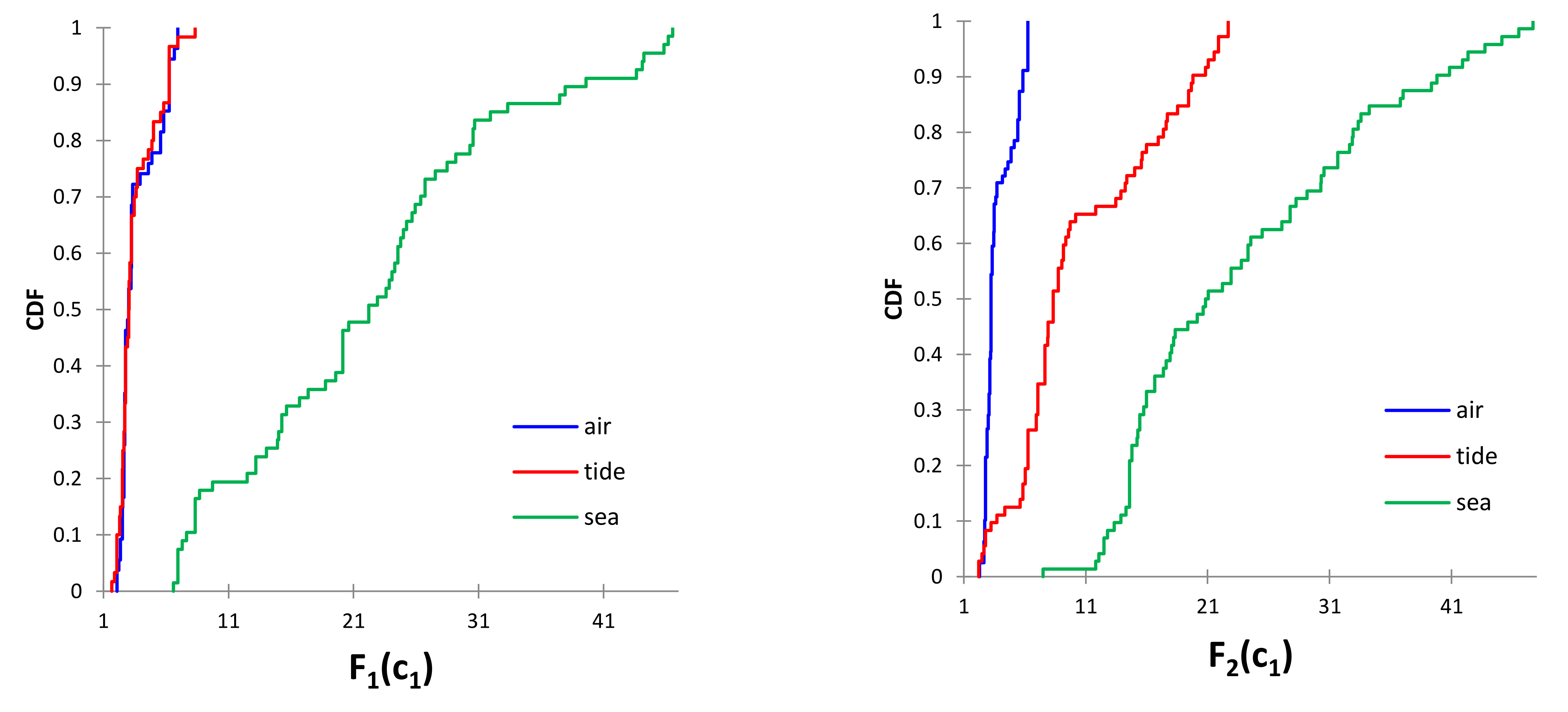
It is well known that a two-tailed KS test can be performed to compare two empirical distributions [63]. Thus, a comparative pairwise analysis of the behaviour of the alloy influenced by the specified seawater environment was performed using the KS test. Namely, the idea was to gain insight into the similarities or differences in the behaviour of different NiTi alloys in each observed seawater environment. Therefore, three KS tests were performed: The first KS test compared the empirical CDF of alloy NiTi-1 and empirical CDF of alloy NiTi-2 in the air environment; the second test compared the empirical CDF of alloy NiTi-1 and empirical CDF of alloy NiTi-2 in the tidal environment, and, finally, the empirical CDF of the NiTi-1 alloy and empirical CDF of the NiTi-2 alloy in the sea environment were compared in the third KS test.

If the empirical CDFs for the two observed samples are denoted by F1 and F2, then the hypothesis of the two-tailed Kolmogorov–Smirnov tests are defined by:

H₀. 

$F_1\left(x\right)=F_2\left(x\right)$.

Ha. 

$F_1\left(x\right)\ne F_2\left(x\right)$.

In these tests, test statistics denoted as D were calculated as the maximum absolute difference between the two empirical distributions. Appropriate p-values were determined, and they were compared with the chosen significance level $\alpha =0.05$. Test results for all three seawater environments are summarised in

Table 17. Two-tailed KS test results.

	Air Environment	Tide Environment	Sea Environment
D	0.251	0.725	0.180
p-value	0.029	<0.0001	0.189
$\alpha$	0.05	0.05	0.05

.

The computed p-values for air and tide environments were lower than the significance level $\alpha =0.05$, so the null hypothesis H0 cannot be accepted. This means that the empirical distributions of the two NiTi samples are statistically significantly different regarding the corrosion rate in both air and tide environments. The risk to reject the null hypothesis H0, while it is true, was lower than 2.9% when the air environment was observed, while it was lower than 0.01% when the tide environment was observed.

It can be noted that the computed p-value was greater than the significance level $\alpha =0.05$ when the sea environment was observed. Thus, null hypothesis H0 cannot be rejected in the case of sea influence on NiTi-1 and NiTi-2 alloys. This indicates that there is not enough evidence that, statistically, these two alloys were behaving differently in the sea environment. The risk to reject the null hypothesis H0, while it is true, is 18.9%.

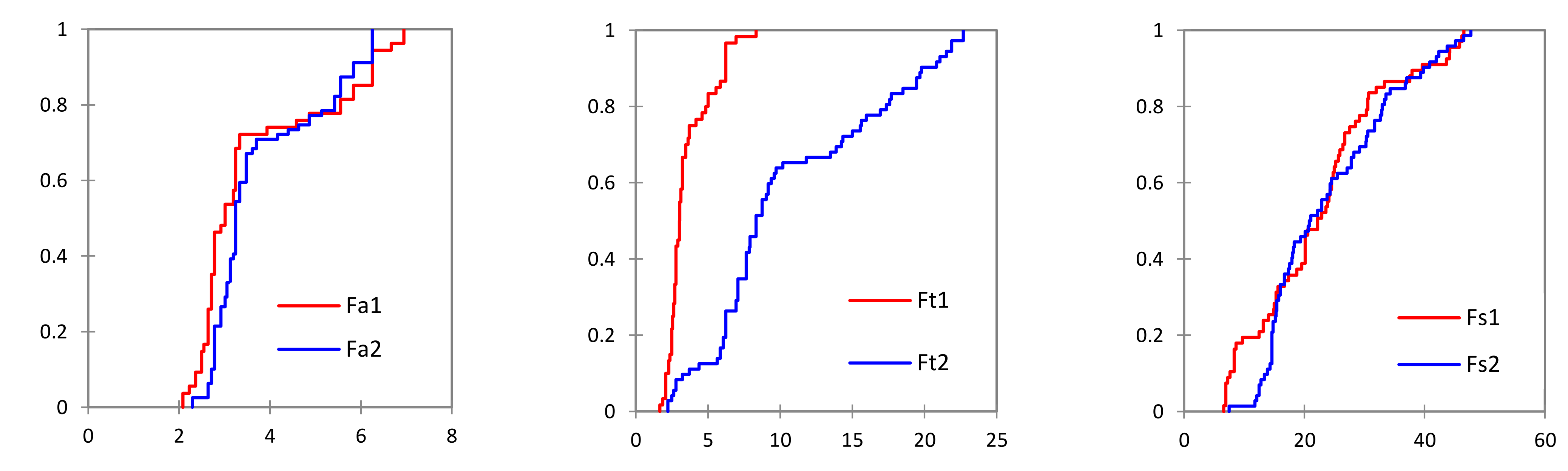
These specific characteristics of NiTi-1 and NiTi-2 alloys in terms of different performance in the air and tide environments and similar behaviour in the sea environment can be examined visually in Figure 18, where the empirical CDFs are compared for the corrosion rates in all three seawater surroundings.

Some additional analysis was conducted motivated by the results of the described KS two-tailed tests. To address the mutually different behaviour of the two NiTi alloys in air and tide environments, and slightly heterogeneous results obtained for the sea environment, sensitive statistical analysis was performed additionally. The goal of this procedure was to quantify the probability difference of the corrosion rate for the two NiTi alloys in each of the three seawater environments.

The corrosion rate difference probability estimate can be calculated under the same assumptions that the corrosion rate can be observed as a random variable, and that samples and empirical results for the NiTi-1 alloy and NiTi-2 alloy can be considered mutually independent. For these purposes, the difference in the corrosion rates were considered of NiTi-1 and NiTi-2 under the air, tide and sea influences. These differences are denoted as $c_a^{\left(1\right)}-c_a^{\left(2\right)}$, $c_t^{\left(1\right)}-c_t^{\left(2\right)}$, $c_s^{\left(1\right)}-c_s^{\left(2\right)}$, respectively.

If X and Y are independent random variables, in some special cases, it is easy to determine the distribution that lay behind the probability difference X-Y (for example, if X and Y are normally distributed random variables [54]). In the following statistical analysis, the corrosion rate of NiTi-1 and NiTi-2 in each of the three seawater environments was approximated with the best-fitting three-parameter distribution specified in Section 2. The theoretical distributions that describe the empirical data of the corrosion processes of NiTi-1 alloy and NiTi-2 alloy best have complex characteristics, making it extremely hard, or even impossible, to find analytical forms of PDF or CDF that will estimate the probability differences of corrosion rate easily. However, some sophisticated numerical methods may overcome these obstacles.

If X and Y are independent random variables given with PDF functions, then the difference Z = X − Y can be determined by the convolution method. The convolution method is a common statistical method used to calculate the sum of two random variables [64,65]. Some random variables X and Y have matching PDFs denoted by $f{}_X\left(x\right)$ and $f{}_Y\left(y\right)$. Then Equation (51) is valid:

$$f_Z\left(z\right)={{\displaystyle \int }}_{-\infty }^{\infty }{f}_Y\left(x-z\right)·f_X\left(x\right)dx={{\displaystyle \int }}_{-\infty }^{\infty }{f}_Y\left(y\right)·f_X\left(y+z\right)dy,$$

(51)

where $f{}_Z\left(z\right)$ represents the probability that the variable Z has a value of z. This probability is determined by all possible pairs of values of x and y whose difference is exactly z. Equation (51) is a representation of one convolution form [66].

Taking into account Equation (51), the independence of the variables X and Y, and the definition for CDF, the corresponding CDF for the random variable Z can be obtained as follows:

$$\begin{gathered} F_Z\left(z\right)=P\left(X-Y\le z\right)= \\ {{\displaystyle \int }}_{-\infty }^z{f}_Z\left(t\right)dt={{\displaystyle \int }}_{-\infty }^{z+y}{f}_X\left(x\right)dx{{\displaystyle \int }}_{-\infty }^{\infty }{f}_Y\left(y\right)dy={{\displaystyle \int }}_{-\infty }^{\infty }{F}_X\left(z+y\right)f_Y\left(y\right)dy, \end{gathered}$$

(52)

For each of the three considered seawater environments it is necessary to replace in Equation (52) the adequate expressions for CDF and PDF of the best-fitted distributions shown in Section 2. For example, if the corrosion rate difference for air is observed, the CDF from Equation (14) and a PDF from Equation (31) have to be incorporated in Equation (52).

In the case of the selected best three-parameter distributions, the combination of the corresponding CDF and PDF functions results in complex integrated functions that are very complicated to integrate, primarily because the exponents and coefficients are decimal values. For the evaluation of such convolutional integrals, it is convenient to apply numerical integration, i.e., numerical convolution. In the background of this algorithm is a very complex recursive procedure involving Cubic spline interpolation and the Five-point Lobotto quadrature formula. A concise description of the numerical convolution algorithm can be found in [67], while a detailed overview of this method is given in [68].

Figure 19 presents the PDF of the NiTi-1 and NiTi-2 alloys corrosion rate differences caused by distinct seawater environment influences. 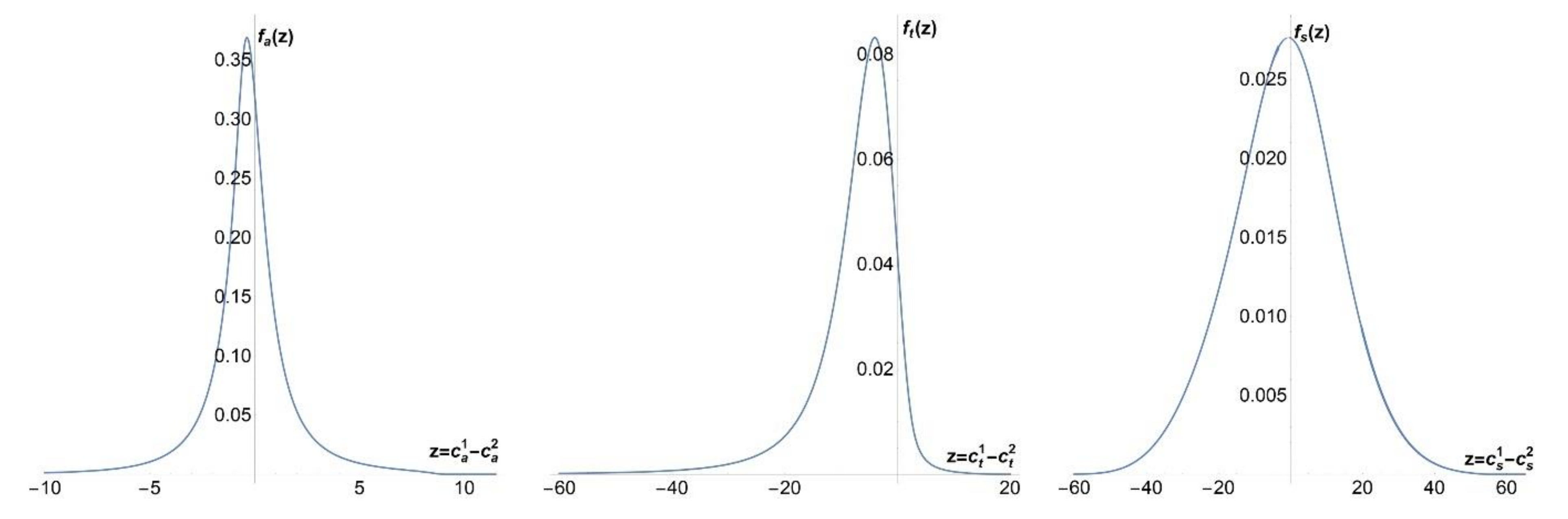The values of the presented probabilities of the differences between the corrosion rate alloys of NiTi-1 and NiTi-2 were obtained by numerical integration of the corresponding convolutions, formed based on the PDF functions of the best-fitted three-parameter distributions, presented in Section 2.

The PDF graph of the NiTi-1 and NiTi-2 alloys corrosion rate differences under air influence, shown at the far left in Figure 19 is very narrow, with a noticeable peak. Based on this, it was concluded that under the influence of air, the probability of a difference in the corrosion rate of these two NiTi alloys was very high in cases where the difference was manifested. The graph is shifted slightly in the negative direction of the x-axis. This fact indicates that, under the influence of air, NiTi-1 alloys generally develop a lower degree of corrosion. The values of the measured differences in the corrosion rate occurred mainly within the interval $\left[-5\mathrm{nm},5\mathrm{nm}\right]$. The PDF function reached its maximum for corrosion rate difference $z=c_a^{\left(1\right)}-c_a^{\left(2\right)}=-0.37\mathrm{nm}$ and the corresponding probability was 0.368778.

In the conditions of the influence of the tide on the corrosion processes, the observed NiTi alloys show the most significant differences, as shown in the PDF graph of the corrosion rate (middle graph in Figure 19). This graph was shifted significantly to the left and tilted slightly to the right. Almost all values of corrosion rate differences are located on the negative side of the x-axis, which means that the NiTi-1 alloy in tidal conditions shows favourable characteristics with respect to the NiTi-2 alloy. Namely, the values of the corrosion rate of the NiTi-1 alloy were almost always lower than the corrosion rate values for the NiTi-2 alloy. However, the associated probabilities were less than the probability of the corrosion rate differences caused by air. The highest probability value was 0.0831721, and it was obtained for the corrosion rate difference $z=c_t^{\left(1\right)}-c_t^{\left(2\right)}=-4.005\mathrm{nm}$.

The PDF for corrosion rate difference is shown in the far-right graph in Figure 19. This graph is almost symmetrical with the y-axis as the axis of symmetry, which is not surprising considering that statistical analysis showed that the NiTi-1 and NiTi-2 alloys behaved similarly from the point of view of the corrosion rate resulting from the influence of the sea. In addition, the values of corrosion rate differences varied more concerning the differences in corrosion rate caused by air, so that the interval from which corrosion rate differences take values was notably wider, and included values between −40 nm and 40 nm. Although the graph shows tendencies of symmetry and centring, more careful observation shows that it is still slightly shifted to the left. The graph reached the maximum value for $z=c_s^{\left(1\right)}-c_s^{\left(2\right)}=-0.6\mathrm{nm}$ with a probability of 0.0276391.

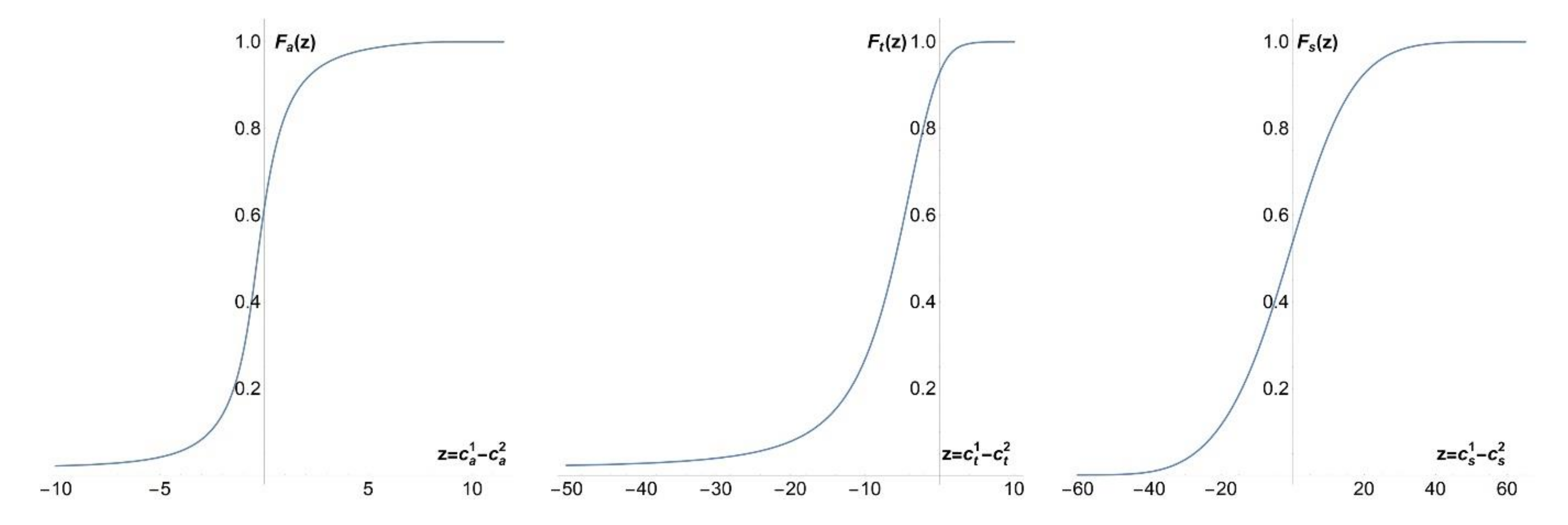
If $F_a\left(z\right)$ denotes the CDF of the corrosion rate differences for the NiTi-1 and NiTi-2 alloys under the air influence, then based on Equation (52) and the numerical convolution algorithm, the following is obtained:

$$P\left(c_a^{\left(1\right)}<c_a^{\left(2\right)}\right)=P\left(c_a^{\left(1\right)}-c_a^{\left(2\right)}<0\right)=F_a\left(0\right)=0.6154.$$

(53)

The same reasoning will yield probability estimates in the case of the observed corrosion rate differences in the case of tide and sea environment influences:

$$P\left(c_t^{\left(1\right)}<c_t^{\left(2\right)}\right)=P\left(c_t^{\left(1\right)}-c_t^{\left(2\right)}<0\right)=F_t\left(0\right)=0.9278,$$

(54)

$$P\left(c_s^{\left(1\right)}<c_s^{\left(2\right)}\right)=P\left(c_s^{\left(1\right)}-c_s^{\left(2\right)}<0\right)=F_s\left(0\right)=0.5368,$$

(55)

where $F_t\left(z\right)$ and $F_s\left(z\right)$ denotes the CDF of corrosion rate differences for NiTi-1 and NiTi-2 alloys under the tide and sea influences. Cumulative density functions related to the corrosion rate differences of alloys NiTi-1 and NiTi-2, $F_a\left(z\right)$, $F_t\left(z\right)$ and $F_s\left(z\right)$, calculated by numerical convolution algorithm, are presented in Figure 20.

In the previous sections it has been shown that NiTi-1 and NiTi-2 alloys behave differently from each other when corrosion processes are observed caused by air and tide. Based on the probability values obtained by numerical convolution and shown in Equations (53) and (54), an additional conclusion was drawn that the corrosion rate of the NiTi-1 alloy was mainly lower than that of the NiTi-2 alloy under air and tidal conditions.

Comparative statistical analysis showed that there was no significant difference in the behaviour of the NiTi-1 and NiTi-2 alloys from the point of view of corrosion processes caused by the sea. However, despite this, based on the numerical convolution and Equation (55), it can be concluded that, even in the sea environment, the corrosion rate values for the NiTi-1 alloy were generally lower than the corrosion rate values related to the NiTi-2 alloy.

4. Discussion

In this research the corrosion behaviour of two nickel–titanium alloys in three different seawater environments was analysed by statistical methods. Empirical data on the depth of corrosion were obtained by the FIB method of measurement after 6, 12 and 18 months of continuous exposure to the effects of air, tide and sea. A database for the corrosion rate of the two observed alloys was formed based on the empirical data.

In the preliminary modelling the corrosion rate was observed as a constant value during the exposure of each alloy to the effects of the seawater environment, but assuming that corrosion begins to develop immediately after the sample is exposed to the environment. Based on this, adequate linear corrosion models were formed for each NiTi alloy and each environment. Three important assumptions were made in this preliminary modelling:

• NiTi-1 alloy behaved similarly in conditions in which the dominant influence on the corrosion rate is air or tide, while corrosion processes were significantly more pronounced in conditions of exposure to the sea;
• NiTi-2 alloy did not show similarities from the point of view of corrosion processes in any of the three observed environments;
• NiTi-2 alloy behaved completely differently from the NiTi-1 alloy in all three environments.

These assumptions were verified further by appropriate statistical analyses, because their confirmation would prove that, in addition to the composition of the alloy and the properties of the corrosive environment, the production method had a great influence on the corrosion behaviour of each observed NiTi alloy.

It is generally known that corrosion processes are influenced by various factors that have uncertain characteristics. To capture this property of the corrosion rate, in the following statistical analysis, the corrosion rate was observed as a continuous real-valued probability variable. Normality tests have shown that empirical data do not follow a normal distribution, and that more complex distributions need to be considered. By detailed analysis of the data and preliminary testing, it was found that the two-parameter continuous distributions were not adequate for modelling such complex corrosion processes of the observed NiTi alloys. Therefore, 27 three-parameter continuous distributions were selected for further consideration. In the process of fitting three-parameter theoretical distributions into a probabilistic empirical corrosion model, statistical analysis revealed the continuous distributions that best reflect the shape, scale and location of the empirical data. The following theoretical distributions were detected as the most favourable for describing the corrosion processes of the two observed alloys:

• For air influence, three-parameter Log-Logistic and Burr distribution;
• For tide influence, Burr and three-parameter Log-Logistic distribution;
• For sea influence, Generalised Extreme Value and General Pareto distribution.

The positive tail of all the selected distributions extended out quite a long way, whereas the negative tail stopped near zero. As distributions with positive tails are detected to fit data in the best way, it can be concluded that the highest corrosion rate values are usually much higher than typical corrosion rate values, whereas the lowest corrosion rates are seldom much less than typical corrosion rate values. In the case of the dominant influence of the sea or tides, especially with the NiTi-1 alloy, high values of material wear due to corrosive processes were observed frequently.

The main findings of the comparative analysis of the two NiTi alloys were:

• The corrosion processes of the observed alloys were statistically significantly different if the samples came under the influence of air, and they also differed significantly if the corrosion processes developed under the influence of the tide;
• The largest differences in corrosion rate values occurred under the influence of the tide;
• In all three environments, the corrosion rate values of the NiTi-1 alloy were generally lower than the corrosion rate of the NiTi-2 alloy. This corrosion behaviour of the NiTi-1 alloy can be explained by its homogeneous microstructure (see Figure 2). However, more extensive studies and additional methodologies are needed to draw a definite conclusion about the corrosive behaviour quality of these two NiTi alloys. In this way, an insight into the deeper layers of the alloy would be obtained, as well as into their detailed chemical structure, which would increase both the empirical database and the statistical significance of the obtained results.

The corrosive processes of the two observed NiTi alloys under the influence of the tide developed as expected. It is well known that the tide is the most aggressive of all the analysed environments, because the alloy is exposed alternately to wet-dry conditions and the effect of waves. The smallest changes in the corrosion behaviour of the two alloys were registered in the sea. This can be interpreted by the fact that the seawater is a corrosive environment that, during the examined time interval, suffers the least changes, primarily in temperature (and humidity) concerning the other two tested environments.

5. Conclusions

Summarising all the previous findings, it becomes clear that the statistical analysis proved the expected fact that the technological process of production of NiTi alloys affects their favourable characteristics significantly from the point of view of reducing the susceptibility to the corrosion process.

Analysis of linear models of the corrosive behaviour of the two observed NiTinol alloys shows significant differences in the corrosive behaviour of these alloys. Namely, the linear models suggest the following facts:

• NiTi-1 alloy corrodes significantly faster in conditions of exposure to the sea;
• NiTi-1 alloy shows similar corrosive behaviour under the influence of air and tide;
• The corrosive characteristics of the NiTi-2 alloy differ significantly when samples come out affected by different marine environments;
• In all marine environments, the NiTi-2 alloy behaved completely differently from the NiTi-1 alloy.

The corrosive behaviours of both NiTinol alloys are very complex, and cannot be characterised with Normal distribution or with two-parameter continuous distributions. Consequently, in the process of fitting distributions, it is necessary to consider three-parameter continuous distributions, that can describe the empirical data adequately. The Kolmogorov–Smirnov goodness-of-fit test revealed the following continuous distributions as the best ranked three-parameter distributions for the three observed seawater environments:

• NiTi-1, air influence, three-parameter Log-Logistic distribution;
• NiTi-2, air influence, Burr distribution;
• NiTi-1, tide influence, Burr distribution;
• NiTi-2, tide influence, three-parameter Log-Logistic distribution;
• NiTi-1, sea influence, Generalised Extreme Value distribution;
• NiTi-2, sea influence, General Pareto distribution.

A comparative analysis of the behaviour of two NiTinol alloys shows the following characteristics of their corrosive processes:

• Statistically significant differences were observed when samples were exposed to air or tide;
• The largest differences in the depth of corrosive changes in NiTinol alloys occurred in samples exposed to the effects of the tides;
• The NiTi-1 alloy showed a tendency of reduced corrosive processes in relation to the values of corrosion depth in the NiTi-2 alloy in all three observed seawater environments.

However, although the three-parameter theoretical distributions proved to be adequate for modelling the corrosion process in the observed alloys in all three environments, nonlinearities were detected, especially in the tails of the fitted distributions. Therefore, it is necessary to focus future research on the analysis of nonlinear models that will take into account the stochastic side of the corrosion process. To conduct an analysis of this type, it is necessary to form bigger databases with even more extensive empirical samples, which would allow increasing the statistical significance of the findings. In this study, only FIB analyses were performed on a NiTi-1 alloy (disk surface) and NiTi-2 alloy (on a flat bar surface). Using additional complementary methods, such as X-ray fluorescence analysis, auger electron spectroscopy, X-ray mapping or X-ray photoelectron spectroscopy, further conclusions can be drawn with high reliability about the actual changes of the alloy under the influence of different seawater environments, as well as their comparison regarding quality.