1. Introduction
One of the most discussed recent research topics in wireless technology and smart home applications is human activity recognition (HAR), and there are numerous applications such as health care, ambient assisted living, and children and elderly people monitoring systems.
In 2017 in 22 Western European countries there were reported at least 8.4 million injury cases due to falls. Most people who sought medical help were people aged 70 and older. According to [
1] 54,504 of them had fatal falls. A total of 5667 per 100,000 people in the age range 70–74 years and 47,239 per 100,000 people in the age category of 95+ years required medical help due to injuries. However, these numbers are greatly underestimated, since not every elderly person reports every fall. As a result, delay of medical assistance can worsen the condition of hidden wounds and make a person more vulnerable to future falls. Once the person falls, the probability of a person falling again doubles [
2]. In some cases, immediate help is a matter of life and death because elderly people might lie helpless and unconscious at home for hours before they are admitted to the hospital, as they are not able to call for help. HAR for motion detection and human fall detection could benefit the medical staff in hospitals, elderly people care houses and people with paralysis, epilepsy, hypoglycemia diabetic diseases, and others. Detection of human activities and classification of these activities are challenging tasks. In recent years, devices like the Closed Circuit Television (CCTV) monitoring systems and wearable devices are mostly used to accomplish these tasks. Recent advancements in Wi-Fi-based machine learning solutions could become an alternative and simplified solution for usability and personal privacy concerns [
3].
Apart from this, HAR has excellent potential for smart home applications. Instead of using infrared or proximity sensors to control an individual electronic device, the Wi-Fi-based solution could be integrated to control all the devices in the smart home or nursing homes [
4]. Another potential application area could be crowd counting and better management of the public places crowd, shopping malls, or open markets in a situation like Coronavirus disease (COVID-19), or the situation where emergency response is required.
In wireless communication standard 802.11, the channel state information (CSI) contains useful information in a Wi-Fi packet’s preamble. It consists of information about the amplitude attenuation and phase shift of the transmitted signal alongside the transmitted path. Analysis of CSI data can give information about surroundings and variations over time while the Wi-Fi signal is being transmitted [
5]; for the reader’s convenience, we have included a brief introduction to the subject in
Section 5. The HAR system can act as a virtual eye for monitoring and triggering a responsive alarm for quick action emergencies. These days, many elderly people become victims of such instances where quick assistance is critical as falling from stairs, slipping in the bathroom, etc. Wireless HAR can be an alternative solution to video surveillance, as it will protect privacy.
There is some CSI-related work already performed in this area by Francesco Gringoli et al. and Matthias Schulz et al. using the Nexmon tool [
6,
7,
8]. The full control and access to wireless hardware’s CSI information are not always possible as most wireless chip manufacturers keep these features private and inaccessible to the outer world. Alternatively, the software solutions and hardware solutions provided to get access to this CSI information are expensive. There are some tools based on Linux, which can access the CSI of a channel up to 40 MHz [
9,
10]. Interestingly, the open-source Nexmon tool used in this work can analyze up to 80 MHz [
7].
Recent work [
11,
12] used Intel Wi-Fi Link (IWL) 5300 Network Interface Card (NIC), which supports 802.11n standard. In that work, the CSI information was used to classifying human activities by preprocessing the data with the use of discrete wavelet transform (DWT), principal component analysis (PCA), power spectral density (PSD), SVM, and LSTM recurrent neural networks implementation [
12].
In our work which is mainly based on the master theses of some of the authors, we explore CSI data acquisition possibilities using Nexmon with a Raspberry Pi 3 B+, Pi 4B [
13], and Asus RT-AC86U based platform [
14,
15] and human activities classification using machine learning algorithms with a focus on practical deployment. We conducted three different types of experiments not only on different hardware but also in different environmental contexts and using different algorithms.
The paper’s main contribution is to solve the HAR problem by using inexpensive hardware without the necessity of humans wearing any devices whilst achieving accuracy on par with or better to published methods. The approach is first acquiring CSI data from inexpensive networking hardware and then applying machine learning algorithms to distinguish between different activities. Even if there are differences in the used hardware, the environmental contexts, and the algorithms, all approaches solve the HAR problem with similar and good accuracy. This is encouraging for practical deployments.
2. Problem Statement
2.1. Objective
There exists a large amount of research on activity detection using different devices. For a comprehensive overview, see the survey [
10]. Some of them are designed to be worn on the body and others to be installed in the environment the person is staying in. For continuous observation of people, a contactless device is considered to be a better solution to avoid situations when a person forgets to use the device. Additionally, the contactless solution can be accepted better among the elderly. Depending on the illness, people can take the device off the body thereby making observation inaccurate. An example can be people having dementia who might remove clothes and as a result, removing any device attached to the body [
16]. For this purpose, the ideal solution is to use a Wi-Fi signal. Compared to the related work on HAR, where the human activities are recognized using wearable devices such as smartwatches, arm and chest bands [
17], and using vision-based devices for 3-D human body positioning with Xbox360 vision aids [
18]. HAR using Wi-Fi CSI information is a complicated task, affected by numerous surrounding parameters, such as multipath reflections of Wi-Fi signal in the nearby environment where the activities are performed, temperature and humidity of the air, influence the amplitude, and phase shift of the received signal. The clock of NIC and its power management mode with the automatic gain control (AGC) influence the signal strength based on the network traffic significantly [
19]. The various manufacturers and their different hardware architectures and firmware add up to make CSI information for HAR more difficult to generalize the wireless-based solutions. Considering the above challenges, the Wi-Fi-based human activity recognition techniques and the classification of activities is demanding.
Contemplating the above challenges in wireless-based HAR, this work aims to work with the open-source Nexmon CSI tool on Raspberry Pi hardware [
20] with NIC Broadcom
® BCM43455c0 and Asus RT-AC86U routers. The work focuses on extracting the CSI information for EMPTY, LYING, SIT, STAND, SIT-DOWN, STAND-UP, WALK, and FALL in the indoor Line of Sight (LOS) scenarios using Raspberry Pi 3B+, Pi 4B, and Asus RT-AC86U and then classifying the activities applying machine learning algorithms, support vector machine (SVM), and long short-term memory (LSTM). In particular, we performed the experiments depicted in
Table 1, the details are covered in the following section.
In the following section, we refer to the experiments as Experiment i (), where Experiment 1 has two variants, referred to as 1.1. and 1.2, respectively. In Experiment 1.1, outliers were removed from the CSI values using Hampel Identifier, then DWT was applied to denoise the signal and PCA to reduce the dimension of the dataset. Then features were extracted from the preprocessed data to use in SVM and LSTM to classify activities. In the case of Experiment 1.2, Hampel Identifier and Discrete Wavelet Transform were applied as in Experiment 1.1, however, PCA and feature extraction were omitted.
2.2. Scope
The paper’s primary work scope was to evaluate possibilities for using cost-effective and less complicated hardware (Raspberry Pi) for human activity recognition using CSI information of the Wi-Fi signal. Following is the primary outline of the work.
We patched the Wi-Fi driver of the Raspberry Pi 3 B+, Pi 4B, and Asus RT-AC86U with the stable version of open-source Nexmon firmware.
We extracted the indoor environment’s CSI information for the following activities on frequency bandwidth 20 MHz, 40 MHz, and 80 MHz (note, that not all activities were performed for all experiments, see
Section 9)
- –
EMPTY
- –
LYING
- –
SIT
- –
STAND
- –
SIT-DOWN
- –
STAND-UP
- –
WALK
- –
FALL
We made a quantitative features dataset by denoise the CSI data for possible outliers, performed principal component analysis (PCA), and extracted a feature matrix.
We used the feature matrix for machine learning algorithms such as SVM classifier.
We denoised raw data and preprocessed CSI data matrix for LSTM.
The data was divided into a random 80 to 20 ratio for training and testing. The final results were mapped into confusion matrices for comparison to evaluate the feasibility of Raspberry Pi and Asus RT-AC86U hardware for a cost-effective and less complicated alternative with acceptable accuracy.
We compared the obtained results by one-to-one comparison for the above-mentioned machine learning algorithms, and a relative comparison of the obtained results with related prior work performed using IWL 5300 NIC [
12].
CSI data were classified using machine learning algorithms and recurrent neural networks (RNN).
2.3. Contribution
The following hypotheses were tested:
For human activities classification, where data is collected in some controlled environment with Raspberry Pi and Asus RT-AC86U hardware, both hardware should produce relatively comparable similar results and also be consistent with or better than as published in related work [
12] on evaluation with machine learning algorithms.
SVM can perform as well as LSTM if the data is properly denoised and a careful feature design takes place.
For LSTM, it is not necessary to preprocess the raw data to achieve state-of-the- art performance.
Up to the best of our knowledge, the results obtained are the first comprehensive HAR results using the Nexmon tool. In particular:
The results achieved were consistent across the three experiments, including different setups and different algorithms. The achieved classification results were relatively similar with both hardware, i.e., Raspberry Pi and Asus RT-AC86U router, in different environmental conditions and for different sets of activities.
The obtained results outperformed previously published results, see the remarks in
Section 3 and the discussion of the results in
Section 9.
The SVM performance is similar to LSTM. However, it requires a careful data preprocessing.
3. Related Work
As HAR is getting widely used, there are many studies on this topic. In 2017 Wang et al. developed a system called Wi-Fall mainly for detecting falls using Wi-Fi CSI data [
22]. In addition to fall, the following activities were analyzed: walking, sitting down, and standing up. These activities were performed in three different locations as chamber, laboratory, and dormitory. Activities were collected using three transmitting and three receiving antennas, which means nine streams were analyzed. As a first step anomaly detection algorithm, more precisely local outlier factor (LOF) was performed. The main idea of the LOF algorithm is to first calculate the density of a point and its k-nearest neighbors and then compare the density of each point with its neighbor’s density. If the density of a point is much smaller than its neighbor’s, then the point is considered to be an outlier. In cases when the majority of streams had outliers, this activity was considered an anomaly. After anomaly detection, singular value decomposition (SVD) was performed. It was observed that the first three samples of the SVD matrix can describe most characteristics of the whole matrix, so the three best eigenvalues were extracted for use in classification. As a classification technique, two different classification algorithms were used. First, a one-class support vector machine (SVM) was utilized to detect falls. The following features were extracted for the SVM classifier:
Normalized standard deviation
Offset of signal strength
Period of motion
Median absolute deviation (MAD)
Interquartile range
Signal entropy
Velocity of signal change
As a result, the precision of fall detection was from 83% to 96% depending on the location of the performed fall and the false alarm rate was from 11% to 18%.
To detect other activities besides fall, random forest was used. With random forest classification, precision increased and became 89% to 98% with false alarm rate from 10% to 15%.
In 2019 Ding et al. [
23] suggested Wi-Fi CSI based HAR using Deep Recurrent Neural Network (HARNN). The idea of their approach is to extract features for Recurrent Neural Network (RNN) training and recognize the activity. This work consists of four main parts:
The first module is used to detect whether any activity was performed. This decision is made by a two-level decision tree that uses variance and correlation coefficient of raw data. If the decision tree detects any activity, the next module is executed. The second module is responsible for denoising data. The feature extraction module is later performed on denoised data where two features are extracted, namely channel power variation in the time domain and time-frequency analysis in the frequency domain. The last module consists of an LSTM that is trained with extracted features to recognize the activity. The following activities were analyzed: running, walking, standing, sitting, crouching, and lying. Activities were collected using Intel 5300 NIC together with CSI Tool [
21]. As a result, the average accuracy of all the above-mentioned activities is 96%.
Recently, convolutional neural networks (CNNs) have been applied together with bidirectional long short-term memory (Bi-LSTM) for classification of human activities including fall [
24], achieving an overall accuracy of 95% to 98%. In [
12] similar results have been obtained (with an accuracy of 100% for FALL which was obtained with a multi-staged approach using two different SVMs for removing false positives).
While the majority of the research is still using Intel 5300 NIC together with the CSI Tool, latest research was done in 2020 on activity recognition [
25] using Raspberry Pi and Nexmon firmware to extract the CSI data. The following activities were collected: nothing, stand-up, sit-down, get into bed, cook, washing dishes, brush teeth, drink, pet cat, sleeping, and walking. The only preprocessing step that was performed on these activities was a low-pass filter. As a classification model DeepConvLSTM model was implemented in Python using a deep learning API called keras. As a result, the activity recognition precision for the above-mentioned activities varies from 66% to 100%. For similar activities such as sit-down and stand-up, the precision was 66% and 68% respectively. For pet cat was 82%, however for all the other activities, the accuracy was higher than 92%. The overall accuracy of the model was 92%.
In this paper, for the best performing models, i.e., Experiment 1.2 and 2, we achieved an accuracy of consistently more than 97% (Experiment 1.2 excluding FALL) and more than 96% including FALL—with 100% for FALL itself, see Table 9 for a summary. For any single activity this is as at least as good as the results described above and altogether better. Furthermore, the particularly important FALL activity is perfectly recognized without using a multiplication-stage approach such as in [
12].
4. The Experimental Setup and CSI Data Collection
This section covers the preparation of the experimental setup including the hardware configuration for the Raspberry Pi 3B+, 4B, and Asus RT-AC86U. It also includes a detailed explanation of challenges and workarounds. This section discusses the system’s architecture and propagation model of the LOS scenario and the human activities’ CSI data collection.
For the experimental setup, the data collection was done with a dual-band router Fritzbox (2.4 GHz and 5 GHz), Pi 3B+ and Pi 4B, and Asus RT-AC86U.
4.1. Hardware Detail
CSI is the collection of data that explains how wireless signals propagate from a transmitter to a receiver, which means it is a mode of communicating amplitude and phase-specific data of individual subcarriers over a transmitting and receiving antenna pairing in the IEEE 802.11N standard [
26]. There are exclusively some manufacturers who make this CSI data available to practitioners. The design of standardized CSI implementation was to control the connection quality. As commercial CSI solutions have been becoming more convenient, numerous comprehensive nonstandard CSI applications have become relevant. For the experimentation, an NIC Broadcom BCM43455c0 and Asus RT-AC86U router were used. Both NICs support the IEEE802.11n/ac standard with MU-MIMO, making it suitable for the frequency band of 20 MHz, 40 MHz, and 80 MHz. On 40 MHz, there are 128 subcarriers; 108 for data, 6 for the pilot, and 14 as null subcarriers. For the duration of data collection, each packet contained the data of all the 128 subcarriers. However, in reality only 114 subcarriers are useful for HAR on Pi NIC. Raspberry Pi official operating system (OS) version Raspbian Buster Kernel v4.19.97 was used on Pi 3B+ and Pi 4B. The default kernel version loaded with the Wi-Fi BCM firmware version does not support the monitor mode to capture the CSI data. The default drivers of NIC by the manufacturer do not enable the monitoring mode functionalities for the end-users.
Another two experiments based on Asus RT-AC86U frequency band of 80 MHz are used in entirely different surroundings with 256 subcarriers. In these experiments, the frequency of 5 GHz was chosen since it has less interference than 2.4 GHz [
27,
28]. One of the Asus RT-AC86U routers is configured to be an access point (AP), and the second one a CSI extractor that has patched with Nexmon firmware which enables the extraction of the CSI data. Additionally, Intel NUC was used that acts as a sender to generate the traffic by sending ping packets to the AP, then AP replies with a pong packet back to the sender. The CSI extractor then captures and extracts CSI data for each pong (see
Figure 1).
4.2. Firmware Patch
4.2.1. Raspberry Pi
Raspberry Pi’s monitoring mode needs to be enabled using the Nexmon patch for BCM43455c0 NIC to capture CSI data. The stable patch can be cloned from the Github directory
https://github.com/seemoo-lab/nexmon [
7].
There were some instabilities with the latest released patch 7
_206 at Nexmon GitHub [
7] encountered, some of the major instability issues were as follow:
Pi 4 automatic loading driver after reboot #437
Unable to change to channels on 80 MHz bandwidth on Pi 4 #434
airodump-ng not working with Pi 4 and 7_45_206 #433
Removing firmware channel restrictions #443
Pi 4 cannot collect CSI packets #448
Corrupted captured data on RPi4 4B #444
0 packets captured #62
Problem with sending frames in 5 GHz channels (RBPi 4) #425
Due to the instability problem faced in patch 7_45_206, the older stable Nexmon patch BCM43455c0 with version 7_45_189 on Rasbian OS Buster Kernel v4.19.97 was used for the experimentation.
The patched firmware enabled the NIC to steer on the desired channel and bandwidth as supported by the geographically selected region. The Nexmon’s monitoring mode enabled the dump of the selected channel’s CSI information with the selected bandwidth.
4.2.2. Asus RT-AC86U Router
The hardware details covered in
Section 4.1 apply to the Asus RT-AC86U router as well. The Nexmon CSI tool allows extracting the CSI data on the Asus RT-AC86U router, which has Wi-Fi chip
BCM4366c0. The Nexmon patch for Wi-Fi chip
BCM4366c0 with
version 10_10_122_20 we used was cloned from the Github repository
https://github.com/seemoo-lab/nexmon_csi [
7].
4.3. Hardware Tuning and Firmware Patching Problem
As highlighted in the above section, there were some common problems encountered.
Inability to change the channels on 80 MHz bandwidth on Pi 4 #434: Many community members have reported this, and the reason for it was region-specific channel allocation in 802.11ac. To fix this problem we configured the channels and respective bandwidth for the European region as listed in and add the desired channel to the “regulations.c” file of the firmware patch.
The second most common issue was 0 packets captured #62: This happens either if the configured channel’s monitoring mode or the router channel configuration is different from the monitoring device.
The other common reason for it is that if the data traffic is overloaded to the configured channel bandwidth, the channel would switch to higher bandwidth on the router because of frequency hopping. Similarly, the Nexmon patched hardware also auto-tunes itself on an available frequency spectrum regardless of the configuration. In the 802.11 standards, the “listen-before-talk” protocol has always been used, where segmentation in the transmitting medium is an essential component of the synchronization mechanism. This enables the co-existence of the channels in the same space by many access points. The BSSID adapts dynamically bandwidth per frame, which is one of the elements of the 802.11ac protocol. It helps achieve the best signal bandwidth and power steering based on the throughput requirement [
29]. To sort out the frequency hopping challenge, constant monitoring of the traffic on the router is required, and maintaining the data traffic as per
Table 2 may help.
4.4. Activity Environment Depiction
For the CSI data collection, rooms of size of approximate 4 m × 4.5 m were used.
The experimental architecture for Experiment 1 is depicted in the
Figure 2a, the data was collected with LOS. There were four activities performed with LOS: EMPTY, STAND, SIT and WALK.
Experiment 2 was performed in a room of size 3.5 m × 4.5 m that is illustrated in
Figure 2b. The distance between transmitter and receiver is around 5 m. In this experiment data for the following activities were collected: WALK, SIT, STAND, SIT-DOWN, STAND-UP, and FALL as a significant additional activity. These activities were performed in different parts of the room to avoid dependence of the activity recognition from the location of the performed activity. The area in
Figure 2b with green color highlights the area where activity WALK was performed, with color blue depicts the area where activities SIT, STAND, SIT-DOWN, and STAND-UP were performed, and with yellow marked the area where the activity FALL was performed.
Figure 2c demonstrates the room layout of Experiment 3. The size of the room is 4.5 m × 5 m. In this experiment, the data were collected for five activities: EMPTY, LYING, SIT, STAND, and WALK in the LOS scenario. All five activities were performed in different parts of the room.
The experimental setup for HAR experiments involving fall detection, in particular, was evaluated by the security officer of the Frankfurt University of Applied Sciences, and a risk assessment was established with assistance from a medical doctor classifying our study as a HAR experiment in accordance with the ethical principles of the Declaration of Helsinki [
31].
5. Propagation Model of Radio Signal
As the CSI data is significantly altered based on human activities, let us consider the time-variant model of the Wi-Fi signal propagation in an indoor environment. For the reader’s convenience we briefly summarize the signal theoretic foundations of the propagation model used and refer to [
5,
28] for further details.
Human activities and their effect on Wi-Fi signals propagation is shown in
Figure 3. Assuming LOS scenario, as shown in
Figure 3 with the propagation path
and multipath scattering propagation along the path
to
. The receiver power
can be described using the Friis transmission Equation (
1) as follows:
where
is the wavelength and
is the transmitter gain,
receiver gain, and
transmitted power [
32]. As the distance
varies w.r.t. time (t) and the human positioning, the received signal’s PSD varies as represented in Equation (
2)
where
and
.
While analyzing HAR based on signal strength alone is possible in principle (see e.g., [
33]) , much more fine-granular data than signal strength is available, namely channel state information (CSI). In the sequel we closely follow the notation from [
34]. Assuming
M antennas and denoting the OFDM symbol of the sender as
,
, where
is the symbol duration,
is the subcarrier spacing, and
is the modulated information onto the
nth subcarrier [
5], then the
lth baseband received signal vector
, containing the signals received is
where
and
L is the number of snapshots taken, the vector
is modeling additive noise for every antenna and
is the complex attenuation along the signal path
q. The
mth entry
of the array response vector
is the response of the
mth antenna to the
qth path arriving from angle
and depends on the antenna geometry.
Substituting into (
3) and sampling the received signal at rate
N times the symbol rate
, i.e., at time instants
, the received signal vector becomes (
denoting the sampled
)
Collecting
N samples and applying
N-point discrete Fourier transformation, results in
The knowledge of
can now be obtained from the network chip set (Nexmon) because it can be calculated from the known training symbols and the received data as
where the channel measurement noise at subcarrier
n is expressed by
,
.
Fundamental to applying CSI to HAR is the fact, that
in (
6) contains geometric information such as the AoA and the arrival time (time of flight or ToF) that is heavily influenced by human activities. Henceforth, knowing
enables one to learn about the activities encoded implicitly into
and henceforth enables HAR. Furthermore, instead of just a single received power
, we have data for every subcarrier (30 to 256 depending on the number of subcarriers) available; thus, instead of a single real number, we have 30 to 256 complex numbers available for analysis. Therefore, the CSI data are much richer and finely granular and their variation supports the different activity classifications.
6. CSI Data Collection
For the CSI data collection, it is necessary to enable monitoring mode on the receiver using Nexmon patched firmware and using the nexutil utility tuning the NIC on the same channel and frequency band as the used router and transmitter. The detailed guide is available on the Nexmon GitHub repository
https://github.com/seemoo-lab/nexmon or
https://github.com/seemoo-lab/nexmon_csi [
7] for the CSI data collection.
In another experiment with Asus RT-AC86U, the experimental setup was similar, where Intel NUC was used as TX without patching and Asus RT-AC86U as RX in monitoring mode on 80 MHz with patched Nexmon firmware.
For each activity, the Raspberry Pi 3B+ without patching any firmware was used to create some network traffic with UDP packets. Another Raspberry Pi 3B+, Pi 4B was configured at 40 MHz at channel 36 (the European region selected for the geographical area) in monitoring mode with patched firmware. A Fritzbox dual-band router was used as a Wi-Fi network bridge at channel 36 with 40 MHz bandwidth with a spectrum of 5 GHz frequency band. There was no patching of the firmware done on the Fritzbox router. It acts as the Wi-Fi media between transmitter Pi and receiver Pi.
After enabling the monitor mode, whenever there was traffic on the network, the CSI data could be captured using the user datagram protocol (UDP) packets with the sender address as 10.10.10.10 and broadcasted packets to the destination address 255.255.255.255. Using the tcpdump tool or Wireshark, the CSI data packets were dumped into the .pcap files for later analysis.
6.1. Challenges Faced for the CSI Based HAR Techniques
There are several challenges to using the collected CSI information for the classification of activities. Firstly, CSI data provides the Wi-Fi signal variations caused by human activities, white noise, and variability in the surrounding events other than unplanned human activities. These factors were responsible for making CSI raw data inappropriate to use directly for classification using machine learning. Numerous precondition and denoising techniques were used to make the data fit for use. These techniques are discussed in detail in
Section 7. Secondly, the presence of pilot and null carriers in the channel, which gives the trend of constant slope and a common characteristic to all the collected data irrespective of the activities, make it difficult for machine learning and classification. These outliers in data are eliminated by identifying and removing such data points. Third, the transitioning of the activity states and sudden peaks due to abnormal change in human actions gives poor segmentation to the activities’ classification. This difficulty arose due to the close resemblance between CSI signatures for different human activities, such as walking vs. standing and sitting vs. standing action. The transition states lead to a high number of false positives. Fast Fourier Transform (FFT) was used to transform CSI data for power spectral density and extract its magnitude.
To denoise the data, Hample filtering and Wavelet signal methods were used. The principal component analysis was applied to extract the feature matrix using moments of order up to fourth. This data was then used for SVM with time-efficient training and classifying the activities. Besides, denoised raw data were used to train the LSTM algorithm with rigorous and deep learning to classify.
6.2. Challenges of Router Frequency Hopping and AGC While CSI Data Collection
As described in
Section 4.2 in the data collection process challenges occurred—two of which are explained below.
The first challenge is frequency hopping/automatic frequency band steering on 802.11ac standard. In fact, this is not a problem for the 802.11ac standard; instead, it is the feature for the better utilization of the frequency spectrum with better data traffic and power management. The method of signal bandwidth and power steering based on the throughput is enabled in most routers to achieve this, a clear-channel assessment approach is used.
- (a)
When Raspberry Pi is configured to 40 Mhz in monitoring mode to capture the CSI data with the Nexmon tool and when the traffic on the network is high enough for the bandwidth on 40 Mhz, then the router automatically hops to use 80 MHz bandwidth, and so the CSI data capturing gets stopped on the configured channel.
- (b)
Similarly, when the receiver is configured in monitoring mode at 80 MHz, if the network traffic exceeds the maximum throughput of 80 MHz, the next hopping for 160 MHz is performed.
The frequency hopping can be avoided by carefully controlling the network traffic and packet transmission on the selected band to avoid exceeding the throughput limit.
The second challenge is automatic gain control (AGC) compensating for the signal amplitude attenuation and adaptive loading applied by the radio modules automatically. Thus, the router modulates the PSD of each subcarrier. The variation in the amplitude occurs for individual subcarriers instantaneously irrespective of the change in the surroundings. It creates sharp spikes in CSI data and a false impression of activities in the experimental setup’s surroundings. In this research work, no counter techniques were implemented to handle this challenge. However, removing the sharp spike outliers and limiting the amplitude maximum range axis by taking the optimal average of the activity countermeasure helped to tame the undesired artificial variations. Alternatively, one could apply CSI calibration techniques described in [
35] or [
36] to compensate for undesired effects of the AGC.
7. CSI Data Preprocessing and Feature Extraction
The CSI data contains information on the subcarriers groups, but not all of them are carrying useful information and the data is very noisy. There are some practical concerns to implement machine learning algorithms on time-series data. The enormous collected data in a controlled environment differ significantly from the real-world scenarios. The collected data need to be refined before feeding into machine learning tools. It has some shortcomings, and it is not free from outliers, unuseful information, and unpredictive spikes in the data, making it unsuitable for direct use for ML and DL algorithms. Several preprocessing techniques are applied to deal with low-quality data, which involve frequency domain representation of data, outlier, and data smoothening techniques.
The data is then further processed for feature extractions and prepared to feed into machine learning algorithms. This section explains the method used to preprocess the CSI data and then use it as input for SVM and LSTM algorithms.
7.1. CSI Data Preprocessing Methodology
7.1.1. Experiment 1: Raspberry Pi 3B+, 4B Using SVM and LSTM
CSI data are affected significantly by noise and ambiguities caused by hardware and firmware. To make the CSI data useful for the machine learning and deep learning algorithms for the classification of human activities, it required some denoising of the data and preprocessing. This section explains the method used to preprocess the CSI data to input SVM and LSTM algorithms. In the first experiment, each packet of the collected CSI data at 40 MHz contained 128 subcarriers in total, where 108 were used for payload, 6 for the pilot, and 14 as null subcarriers. The CSI data was preprocessed, then using this processed data, activity classification using machine learning and deep learning was achieved. First, the collected activity files were segmented into multiple files, where each file contained 150 packets. Second, the data was the denoised and reliable payload of the CSI data extracted by removing the null and pilot subcarriers. In the third step, the fourteen features from each segmented file were extracted for the first two PCA components, and then the feature matrix was fed for the classification using SVM and LSTM.
The preconditioning of the CSI data aims to remove the undesired data packets and subcarriers from each type of human activity raw data file. Each collected raw CSI file was first segmented into an equal size of 150 packets. Each packet contained in total 128 subcarriers, i.e., a raw matrix of
, where
rows and
columns. As not all of them are useful, it is necessary to remove the pilot subcarriers
indexes ±11, ±25, ±53 [
37], eliminating the null subcarriers
indexes 0, ±1, ±59, ±60, ±61, ±62, ±63, ±64, and there are some unchanged subcarriers
indexes ±2, ±3. This removal of the subcarriers gives at the end a matrix of [150 × 104] for each segmented file, see Algorithm 1. This preconditioning is further depicted in
Figure 4 below.
In
Figure 4 the experimental data shows that the peaks at central frequency and waveform of pilot, null and unchanged subcarriers are removed on preprocessing the collected CSI data by eliminating the
= ±11, ±25, ±53 ,
0, ±1, ±59, ±60, ±61, ±62, ±63, ±64, and
±2, ±3 from the raw data.
| Algorithm 1CSI-Data Preprocessing |
- Input:
Raw data as CSIraw, pilot, null and unchanged subcarriers as CSIp, CSInull, and CSIun - Output:
CSI preconditioned as - 1:
← CSIraw - CSIp - CSInull - CSIun
|
7.1.2. Experiments 2 and 3: Asus RT-AC86U Using LSTMs
In the other experiments where Asus RT-AC86U routers with 80 MHz were used, there are 256 subcarriers. In this case pilot and null subcarriers were not removed. For a comparison purpose, two different approaches were applied to scale the CSI data. In the first, the data was normalized and directly used in the LSTM network (Experiment 2). In the second approach (Experiment 3), the data was standardized.
Figure 5 depicts both approaches schematically.
7.2. Hampel Identifier—Outlier Removal for Experiment 1
The CSI magnitude extracted contains noise and outliers caused by the various sources such as adaptive loading and AGC of the carrier frequency offset system nonlinearity. The noise causes spikes in the received magnitude, which can mislead as unexpected activities for the classification and result in inadequate machine learning and testing. The Hampel filter was applied to eliminate outliers and make the CSI data more reliable and smooth.
Using the Hampel identifier, the Hampel filter block detects and excludes the outliers of the input signal. A variance of the three-sigma rule of statistics was implemented in the Hampel identifier, which is effective against outliers. For each input sample, it calculates the median absolute deviation (MAD) of the current sample and neighboring samples of size
− 1)/2 where
is the window length in either direction of the current sample [
38]. The window length equal to 3 was chosen because this window length gave optimum removal of outliers.
Let
be the threshold value and
the standard deviation of current sample. For a current sample
(i), the algorithm worked as follows. It adjusts the window of odd length at the current sample
(i) to calculate the local median for the current sample window of CSI data as depicted in Algorithm 2.
| Algorithm 2Outlier Removal |
- Input:
← local median of current window of (i) - Output:
Outliers removed as - 1:
Compare the current sample (i) with - 2:
ifthen - 3:
- 4:
end if - 5:
|
Thus, when the if condition is true, it recognizes the current sample, , as an outlier and replaces it with the median value else it keeps it unchanged.
It can be seen in
Figure 6 that the outlier peaks and unsymmetrical magnitude variations are reduced compare to the preprocessed data.
7.3. Noise Attenuation Using Discrete Wavelet Transform (DWT) for Experiment 1
The obtained
was free from potential outliers. However, the received wavelet was not smoothed. There are many minor spikes with micro-steps. The plotted CSI looks as depicted in the
Figure 6. The noise comes from micro variations in system nonlinearities, the ambient temperature and humidity in the air [
39,
40].
Discrete wavelet transformation (DWT) is a well-known technique in signal processing [
41]. To reduce the signal distortions preprocessing of the CSI data with wavelets in the frequency domain was carried out. To this we applied the orthogonal wavelet method symlet sym6. There are numerous mother wavelet techniques available such as Haar, Symlet, Coiflet, Mexican Hat, Morlet.
Symlet wavelet sym6 provided the best result with the level of wavelet decomposition “5”. The inherent ability to process signals in different frequencies and levels can be crucial in measuring transmissions’ behavior in different frequency segments. Therefore, it is a relatively simple method to identify the distortion inside the transmission and reduce it. Finally, after applying the DWT denoising technique, the obtained data is cleaned from the anomalies, the reformed waveforms are smoother and free from noise, microspikes, and outliers, see Algorithm 3.
Figure 6 shows an example of the final waveforms for an activity.
| Algorithm 3Denoising |
= 1800 number of files for activities
- Input:
Noisy signal = with - Output:
- 1:
← DWT on () with wavelet decomposition (level = 5) & (wavelet scheme = sym6) - 2:
=
|
7.4. Principal Component Analysis (PCA) as Dimension Reduction for Experiment 1.1
The magnitude of CSI data is now preconditioned, free from the pilot, null, unchanged subcarriers, outliers, and noise. Further, we still have a matrix [150 × 104] for each file, where columns represent 104 dimensions. For each activity, the number of files is 1800, so the total data dimension would become 1800 × . This data is quite significant to use for activity classification. PCA’s main motive is to extract the essential data in a smaller dimension without losing vital information and characteristics. PCA contributes for transforming a large set of variables into a smaller one while the reduced dimension still contains most of the extensive dimension information.
In our case, the first two components represent 75% to 81% of the variance of the data. So the whole dimension of [150 × 104] was reduced to [150 × 2] while preserving vital features. The columns correspond to the subcarriers, and the rows correspond to the values of these subcarriers in each packet.
For each activity, the total dimension of the dataset transformed as [1800 × 150 × 2]. The PCA algorithm that is used for dimension reduction is depicted in Algorithm 4.
| Algorithm 4PCA |
= 1800 number of files for activities
- Input:
extensive dimension matrix = with ( [150 × 104]) - Output:
Principal components as - 1:
[150 × 2] ← PCA on with ( [150 × 104]) - 2:
←
|
7.5. Feature Extraction for Experiment 1.1
After applying PCA, the CSI matrix is used in two different ways for the machine learning algorithms. First, by extracting seven features, namely:
Standard Deviation
Mean Absolute Deviation (MAD)
Median
Mean
Second Central Moment (Variance)
Third Central Moment (Skewness)
Fourth Central Moment (Kurtosis)
Thus for two PCA components, it provides a total of fourteen features for every
data matrix as
which is used in Experiment 1.1 and further used for SVM, see Algorithm 5.
| Algorithm 5Feature Extraction |
= 1800 number of files for activities
- Input:
reduced dimension matrix with [150 × 2] ; - Output:
The features as - 1:
[150 × 14] ← Feature extraction on with ( [150 × 2]) - 2:
← [150 × 14]
|
In the second method, the extracted is used for the LSTM network without extracting any feature matrix for Experiment 1.2.
The block diagram representation of the whole preprocessing is shown in
Figure 7.
8. HAR Classification and Performance Analysis
Numerous classification algorithms are used in the related works for the HAR and classification of these activities; some of the well-known ones are SVM, KNN, and random forest [
3,
11,
12,
42,
43]. In previous sections, CSI data were preconditioned, denoised, and a feature matrix was prepared to classify the activities. This section covers the implemented machine learning and neural networks algorithms used for the human activities classification. There are several algorithm tuning parameters used for optimizing machine learning and neural networks. The achieved results of classifications are also discussed.
8.1. HAR Classification Using Support Vector Machine for Experiment 1.1
Support vector machines are well-known machine learning methods [
44] for classification or regression problems. As in our case, we have multiple classes to classify, a multi-class approach is required.
8.2. Multiclass Classification Using SVM for Experiment 1.1
The SVM is suitable for classification when the data has precisely two classes and is linearly separable. Yet, it becomes unsuitable for the multiclass when the data is not linearly separable because the hyperplane of SVM can divide only for binary classes. Nevertheless, the same principle of dividing the class with hyperplane can be used by clustering the data in multiple clouds and using soft-margin SVM to find the hyperplane of maximal margin within an acceptable tolerance of nonlinear data points on the decision boundaries.
Two different approaches can be used to achieve multiclass SVM classification: One-to-One and One-to-Rest. In the One-to-One approach, every two classes are divided with the hyperplane and by ignoring the rest of the classes. In the One-to-Rest approach, choosing the hyperplane separates one class from all other classes, as shown in
Figure 8.
8.3. Deep Neural Network
An LSTM network falls into the deep neural network class. It uses an input layer and multiple nonlinear processing layers working in parallel, known as the hidden layers. This is inspired by the biological neural network and an output layer; these hidden layers use the previous layer’s output as input. All the layers are connected with nodes, also called neurons. One of the deep learning algorithms is the recurrent neural networks (RNN).
8.3.1. Recurrent Neural Networks (RNN)
RNN is a deep learning network that uses past information and updates its neural network to improve present and future inputs. The unique feature of RNN is the use of hidden states and loops between different states, see e.g.,
Figure 9. RNN uses the weights for learning; it retains the current input state weight and hidden state weight. In simple words, for the sequential classification problems, RNN has a hidden state loopback that retains previous states’ weight and feeds them forward.
It is well-known that, with time, information retention becomes problematic as it suffers from the so-called vanishing gradient problems. RNN uses the loss function, which is the difference between the actual value and the predicted value. This loss function is backpropagated to calculate the gradient and adjust the weights for network learning. Because the gradient adjustment is recursively applied multiple times, the gradient might either explode or vanish [
45]. In both cases, the learning of the network gets worse. To mitigate this problem, LSTM [
46] invented a specialized variant of RNN.
8.3.2. Long Short-Term Memory (LSTM)
LSTM is a deep learning network that uses RNN methodology for learning. The RNN experiences gradient explosion or shrinking in long-term relationships while training, which resulted in low effectiveness and accuracy. LSTM uses additional gates to influence and better guide the next state’s learning to overcome this problem. Gates helps to decide whether the previous state’s output is helpful for the output of the next state or it is better to forget the previous state weights for better improvement of the learning and training.
8.3.3. CSI Data Selection for LSTM for Experiment 1.1 and for Experiment 1.2
For the implementation of LSTM, there were two types of data sets prepared. The first one is as described in the
Section 7.5. For each CSI data packet in Experiment 1.1, 14 features were extracted using the first two PCA components as shown in
Figure 10.
Algorithm 6 used for the LSTM Experiment 1.2 is depicted below:
| Algorithm 6dataset extraction for Experiment 1.2 |
= 1800 number of files for activities
- Input:
- Output:
Data set for Experiment 1.2 - 1:
[150 × 104] ← with @ [150 × 104]
|
In the second approach, the activity file is denoised without PCA, without selectively extracted features, as shown in
Figure 10. Preferably the whole data matrix [150 × 104] which is Experiment 1.2 is used as an input for the training/testing of LSTM. The second approach is used to avoid losing vital features from the data while selecting the 14 features based on PCA reduced dimensions.
8.3.4. LSTM Model Architecture of Experiment 1.1 and Experiment 1.2
For the implementation of LSTM for the CSI data classification, an eight layer network was designed. It involves the following:
One input layer.
Two hidden LSTM layers of 125 and 100 hidden units simultaneously to learn long-term dependencies.
Two dropout layers with 20% neurons dropout for every 10 epochs to avoid the gradient explosion problem and stable learning without any glitches.
Four fully connected network layers, each activity followed by a softmax layer for transforming the weights between 0 to 1.
A classification layer for the activity classifications.
The adaptive moment estimation (ADAM) optimizer uses the lower order moments and gradients of the first order for effective stochastic optimization in the training options [
47] because is computationally efficient, has little memory requirement, is invariant to diagonal rescaling of gradients, and is well suited for problems that are large in terms of data/parameters. As described in
Section 8.2, higher-order moments were not useful for better machine learning and improving the classification. The max epochs size between 40 to 45, a minibatch size of 32, and a validation factor for every 130 to 135 iterations are configured for the best outcome. A gradient threshold set as one and piecewise dropping rate methodology avoids the exploding gradient problem and overfitting. The LSTM network architecture is illustrated in
Figure 11.
8.3.5. Overfitting Problem of LSTM
With the deep learning algorithms, overfitting of the model is a common problem. Overfitting occurs when the model achieves very high accuracy while training but classifies the data inadequately or sometimes drastically fails when exposed to classify new test data. If the training losses decrease but the validation losses increases, that is a sign of overfitting.
Overfitting can be avoided by simplifying the network design. Adding more hidden layers does not always improve the efficiency of the model. Finding a fair tradeoff between the number of hidden layers used, the number of neurons in each hidden layer, and adding the drop-out layers with piecewise dropping of neurons and reducing the learning rate every 10 epochs facilitated better performance of the LSTM network. Another approach is early stopping. If the validation losses start rising and there is a drop in the learning accuracy, it is better to stop network training early. In the
Figure 12 training is early stopped on completion of 34 epochs yielding an accuracy of 98.89%.
8.3.6. LSTM Model Architecture of Experiment 2
The architecture of LSTM model for Experiment 2 can be observed in
Figure 13. This model consists of the following layers:
Sequence input layer, where the input dimension is equal to 256, since the number of subcarriers for Experiment 2 is 256.
LSTM layer with 100 hidden units.
A dropout layer with 40% probability of dropping out the input elements.
Six fully connected layers.
Softmax layer.
A classification layer for the activity classifications.
As an optimizer, the ADAM optimizer with default parameter values was used. A max epoch size of 60 was set, since a higher max epoch size was not giving better results; however, the learning time was increasing. As a mini-batch size, the value of 32 was chosen.
8.3.7. LSTM Model Architecture of Experiment 3
Figure 14 demonstrates the summary of the LSTM model for Experiment 3 (
Table 1). The LSTM layer has 64 units with an input shape of (500, 256), where 500 is the number of packets, and 256 is the number of subcarriers. The next layer is the dropout layer with a 0.5 value to control the overfitting; after that, there is a dense layer with 32 units with an activation ReLU. The last layer of the model is the output layer, which is also a dense layer with activation softmax. The model is compiled with the categorical_crossentropy loss. Additionally, the Accuracy metric is computed during training. The ADAM optimizer is used with a learning_rate of 1
.
Figure 15 demonstrates the exponential decay scheduling for the LSTM model for experiment 3. The learning rate between 1
and 1
has the minimum loss value.
9. Classification Results
9.1. Experiment 1.1: Summary of Multiclass SVM Classification Based on Pi 3B+ and Pi 4B Hardware
Multiclass SVM with the One-to-One approach and with polynomial kernel and error-correcting output codes (ECOC) model is applied to classify the four activities, SIT, STAND, WALK, and EMPTY by using the features mentioned in
Section 7.5 for training the network.
The ECOC method allows a multiclass classification problem to present as a multiple binary classification problem. A box constrains parameter referred to as C = 8.48 is the model’s optimization’s tradeoff parameter. It supports making the class boundaries stricter. The multiclass SVM model is executed with cross-validation of 10 fold to estimate the loss function and validate the training accuracy.
The achieved classification results are presented in
Table 3. The confusion matrix illustrates the recall (diagonal values) and precision after the classification of activities. The multi SVM model accomplished approximately 96% of the training accuracy and the precision achieved between 95% to 98.9% for different classes.
9.2. Experiment 1: Summary of LSTM Classification Based on Pi 3B+ and Pi 4B Hardware
The prepared data sets, first Experiment 1.1 and the second data set of Experiment 1.2, as described in the previous
Section 8.3.4, are fed to the LSTM network. The obtained results are promising. The achieved classification results are presented in
Table 4 and
Table 5. The confusion matrix illustrates the recall (diagonal values) and precision after classification of activities. The precision achieved in Experiment 1.1 with 14 features varied between 88.8% to 96.9%. On the other hand, the precision achieved without extracting the feature data, e.g., Experiment 1.2 was approximately 97% to 99.7%. These achieved results are very satisfactory because in another experiment based on Asus RT-AC86U the produced results were relatively similar when the CSI raw data was processed in a different environment for similar activities.
9.3. Experiments 2 and 3: Summary of LSTM Classification Based on Asus RT-AC86U
9.3.1. Experiment 2: Results after Data Normalization
In Experiment 2 raw CSI data were normalized before training the LSTM model. With normalized data, an accuracy of 96.2% to 100% was achieved. More detailed results for Experiment 2 can be observed in
Table 6.
9.3.2. Experiment 3: Results with Data Rescaling
In this experiment, the CSI was collected based on Asus RT-AC86U. With the data scaling approach for preprocessing, accuracy of 94.1% to 100% was achieved, which is comparable to the accuracy achieved based on Pi hardware.
Table 7 demonstrates the confusion matrix. It can be observed that WALK, LYING, and EMPTY have the highest accuracy. SIT and STAND classes have almost the same accuracy. The possible reason for some misclassification in SIT and STAND can be that both are passive activities and many waveform characteristics were similar in these activities.
9.3.3. Experiment 3: LSTM Model Performance for Different Combinations of Hyper-Parameter
The LSTM model was trained for 100 epochs with the callback early stopping when validation accuracy reached greater than 98%.
Table 8 illustrates the performance summary of the LSTM model with different combinations of hyper-parameters of Experiment 3. Test 1 and Test 5 have similar test accuracy with 98%. Test 5, with learning rate of 1
, reached threshold validation accuracy in 18 epochs, while in Test 1, it took 87 epochs to reach the threshold validation accuracy with a learning rate of 1
.
9.4. Overall Results
Table 9 illustrates the overall performance and achieved results. It can be observed that all the experiments produced relatively similar results with Nexmon CSI data irrespective of the hardware and environment. Note, that the important fall classification is perfect.
10. Conclusions
Many of us have easy access to Wi-Fi-enabled hardware. There are enough radio waves in an indoor environment, which could be useful for HAR applications. Unlike wearable devices or supervised CCTVs, Wi-Fi-based HAR methods do not violate privacy concerns.
This research work was focused on finding the cost-effective, viable hardware option to collect the CSI data and different available hardware options for CSI data collection. The reason is that there are not many options available where the internet provider-owned home Wi-Fi router could be patched with special firmware. The use of hardware such as Raspberry Pi 3B+, 4B, and Asus RT-AC86U was demonstrated as an excellent choice for the CSI data collection using open-source tools such as Nexmon.
The utilization of some of the denoising techniques makes the data useful for machine learning, as explained in this work. CSI information yielded numerous waveform characteristics and acted as an invisible mirror to present the variation that happened in the surroundings unnoticed.
There were two ML algorithms applied for the classification of human activities. SVM with features matrix and the use of LSTM to learn the features automatically performed remarkably excellent.
It can be observed that the HAR classification based on CSI data delivers reliable results irrespective of the hardware used for CSI data collection. The overall performance in accuracy achieved was between 97% and 99.7% (Raspberry Pi) and 96.2% and 100% (Asus RT-AC86U), for the best models.
11. Future Work
For future work, it would be interesting to examine the classification results between automated feature selection and preprocessing techniques that we have used in this paper in more detail. For instance, automated feature selection using deep learning algorithms such as convolution neural network (CNN) would be interesting to explore.
Additionally, for the data preprocessing, the AGC effects removal (using techniques from e.g., [
35] or [
36]) could produce improved results. In the above-performed experiments, the payload was keenly monitored to minimize the effect of AGC. However, it could not be ruled out completely. Firmware may be modified to completely nullify the effect of AGC.
Author Contributions
Conceptualization J.L. and J.S.; methodology J.L. and J.S.; validation B.R.B., M.K. and H.A.; formal analysis J.L. and J.S.; resources B.R.B., M.K. and H.A.; data curation B.R.B., M.K. and H.A.; writing—original draft preparation B.R.B., M.K. and H.A.; writing—review and editing J.L. and J.S.; visualization B.R.B., M.K. and H.A.; supervision J.L. and J.S. All authors have read and agreed to the published version of the manuscript.
Funding
This research was funded by the research support program of Fb2, Frankfurt University of Applied Sciences.
Institutional Review Board Statement
The design of the study was approved by the security officer of the Frankfurt University of Applied Sciences based on a risk assessment with assistance from a medical doctor classifying this type of studies of the university’s research groups as an experiment in accordance with the ethical principles of the Declaration of Helsinki (27 July 2018).
Informed Consent Statement
Informed consent was obtained from all subjects involved in the study.
Data Availability Statement
Acknowledgments
We thank the volunteers who participated in the human activity detection experiments for their time and effort. Their valuable input has lead to beneficial results which were critical to this study.
Conflicts of Interest
The authors declare no conflict of interest.
Abbreviations
The following abbreviations are used in this manuscript:
| AoA | Angle of Arrival |
| AGC | Automatic Gain Control |
| AP | Access Point |
| CCTV | Closed Circuit Television |
| CNN | Convolutional Neural Network |
| CSI | Channel State Information |
| DWT | Discrete Wavelet Transform |
| ECOC | Error-Correcting Output Codes |
| FFT | Fast Fourier Transform |
| HAR | Human Activity Recognition |
| LSTM | Long Short-Term Memory |
| LOF | Local Outlier Factor |
| LOS | Line of Sight |
| MAD | Median Absolute Deviation |
| NIC | Network Interface Card |
| OFDM | Orthogonal Frequency-Division Multiplexing |
| PCA | Principal Component Analysis |
| PSD | Power Spectral Density |
| RNN | Recurrent Neural Network |
| SVD | Singular Value Decomposition |
| SVM | Support Vector Machine |
| ToF | Time of Flight |
| TX | Transmitter |
| UDP | User Datagram Protocol |
References
- Haagsma, J.A.; Olij, B.F.; Majdan, M.; Van Beeck, E.F.; Vos, T.; Castle, C.D.; Dingels, Z.V.; Fox, J.T.; Hamilton, E.B.; Liu, Z.; et al. Falls in older aged adults in 22 European countries: Incidence, mortality and burden of disease from 1990 to 2017. Inj. Prev. 2020, 26, i67–i74. [Google Scholar] [CrossRef] [PubMed]
- O’Loughlin, J.L.; Robitaille, Y.; Boivin, J.F.; Suissa, S. Incidence of and risk factors for falls and injurious falls among the community-dwelling elderly. Am. J. Epidemiol. 1993, 137, 342–354. [Google Scholar] [CrossRef] [PubMed]
- Tan, B.; Chen, Q.; Chetty, K.; Woodbridge, K.; Li, W.; Piechocki, R. Exploiting WiFi Channel State Information for Residential Healthcare Informatics. IEEE Commun. Mag. 2018, 56, 130–137. [Google Scholar] [CrossRef] [Green Version]
- Zou, H.; Zhou, Y.; Yang, J.; Jiang, H.; Xie, L.; Spanos, C.J. WiFi-enabled Device-free Gesture Recognition for Smart Home Automation. In Proceedings of the IEEE International Conference on Control and Automation, ICCA, IEEE Computer Society, Anchorage, AK, USA, 12–15 June 2018; pp. 476–481. [Google Scholar]
- Nee, R.V.; Prasad, R. OFDM for Wireless Multimedia Communications, 1st ed.; Artech House Inc.: Boston, MA, USA, 2000. [Google Scholar]
- Schulz, M.; Wegemer, D.; Hollick, M. Nexmon: The C-based Firmware Patching Framework. 2017. Available online: https://nexmon.org (accessed on 5 August 2021).
- Gringoli, F.; Schulz, M.; Link, J.; Hollick, M. Free Your CSI: A Channel State Information Extraction Platform For Modern Wi-Fi Chipsets. In Proceedings of the 13th International Workshop on Wireless Network Testbeds, Experimental Evaluation & Characterization, WiNTECH’19, New York, NY, USA, 25 October 2019; pp. 21–28. [Google Scholar]
- Schulz, M.; Wegemer, D.; Hollick, M. NexMon: A Cookbook for Firmware Modifications on Smartphones to Enable Monitor Mode. arXiv 2015, arXiv:1601.07077. [Google Scholar]
- Halperin, D. Linux 802.11n CSI Tool. Available online: http://dhalperi.github.io/linux-80211n-csitool/ (accessed on 5 August 2021).
- Ma, Y.; Zhou, G.; Wang, S. WiFi sensing with channel state information: A survey. ACM Comput. Surv. 2019, 52, 1–36. [Google Scholar] [CrossRef] [Green Version]
- Damodaran, N.; Schäfer, J. Device Free Human Activity Recognition using WiFi Channel State Information. In Proceedings of the 2019 IEEE SmartWorld, Ubiquitous Intelligence Computing, Advanced Trusted Computing, Scalable Computing Communications, Cloud Big Data Computing, Internet of People and Smart City Innovation (SmartWorld/SCALCOM/UIC/ATC/CBDCom/IOP/SCI), Leicester, UK, 19–23 August 2019; pp. 1069–1074. [Google Scholar]
- Damodaran, N.; Haruni, E.; Kokhkharova, M.; Schäfer, J. Device free human activity and fall recognition using WiFi channel state information (CSI). CCF Trans. Pervas. Comput. Interact. 2020, 2, 1–17. [Google Scholar] [CrossRef] [Green Version]
- Barrsiwal, B.R. Human Activity Recognition Using CSI Information with Raspberry Pi 3B+. Master’s Thesis, Frankfurt University of Applied Sciences, Frankfurt, Germany, 2021. [Google Scholar]
- Kokhkharova, M. Device-Free Human Activity Recognition Using Channel State Information. Master’s Thesis, Frankfurt University of Applied Sciences, Frankfurt, Germany, 2021. [Google Scholar]
- Adil, H. Human Activity Recognition Using WiFi Channel State Information (CSI). Master’s Thesis, Frankfurt University of Applied Sciences, Frankfurt, Germany, 2021. [Google Scholar]
- Iltanen-Tähkävuori, S.; Wikberg, M.; Topo, P. Design and dementia: A case of garments designed to prevent undressing. Dementia 2012, 11, 49–59. [Google Scholar] [CrossRef]
- Bergelin, V. Human Activity Recognition and Behavioral Prediction using Wearable Sensors and Deep Learning; Technical Report; Linköping University: Linköping, Sweden, 2017; Available online: http://urn.kb.se/resolve?urn=urn:nbn:se:liu:diva-138064 (accessed on 5 August 2021).
- Shotton, J.; Fitzgibbon, A.; Cook, M.; Sharp, T.; Finocchio, M.; Moore, R.; Kipman, A.; Blake, A. Real-time human pose recognition in parts from single depth images. In Proceedings of the IEEE Computer Society Conference on Computer Vision and Pattern Recognition, Colorado Springs, CO, USA, 20–25 June 2011; pp. 1297–1304. [Google Scholar]
- Bloessl, B.; Sommer, C.; Dressler, F. Power matters: Automatic Gain Control for a Software Defined Radio IEEE 802.11a/g/p receiver. In Proceedings of the 2015 IEEE Conference on Computer Communications Workshops (INFOCOM WKSHPS), Hong Kong, China, 26 April–1 May 2015; pp. 25–26. [Google Scholar]
- Raspberry Pi Foundation. 2021. Available online: https://www.raspberrypi.org (accessed on 5 August 2021).
- Halperin, D.; Hu, W.; Sheth, A.; Wetherall, D. Tool release: Gathering 802.11n traces with channel state information. ACM SIGCOMM Comput. Commun. Rev. 2011, 41, 53. [Google Scholar] [CrossRef]
- Wang, Y.; Wu, K.; Ni, L.M. WiFall: Device-Free Fall Detection by Wireless Networks. IEEE Trans. Mob. Comput. 2017, 16, 581–594. [Google Scholar] [CrossRef]
- Ding, J.; Wang, Y. WiFi CSI-Based Human Activity Recognition Using Deep Recurrent Neural Network. IEEE Access 2019, 7, 174257–174269. [Google Scholar] [CrossRef]
- Sheng, B.; Xiao, F.; Sha, L.; Sun, L. Deep Spatial–Temporal Model Based Cross-Scene Action Recognition Using Commodity WiFi. IEEE Internet Things J. 2020, 7, 3592–3601. [Google Scholar] [CrossRef]
- Forbes, G.; Massie, S.; Craw, S. WiFi-based Human Activity Recognition using Raspberry Pi. In Proceedings of the 2020 IEEE 32nd International Conference on Tools with Artificial Intelligence (ICTAI), Baltimore, MD, USA, 9–11 November 2020; pp. 722–730. [Google Scholar]
- Xiao, Y. IEEE 802.11n: Enhancements for higher throughput in wireless LANs. IEEE Wirel. Commun. 2005, 12, 82–91. [Google Scholar] [CrossRef]
- Samantha Albano. WiFi Frequency Bands: 2.4 GHz and 5 GHz. 2019. Available online: https://www.minim.com/blog/wifi-frequency-bands-2.4-ghz-and-5-ghz (accessed on 5 August 2021).
- Goldsmith, A. Wireless Communications; Cambridge University Press: Cambridge, UK, 2005. [Google Scholar]
- IEEE Standard for Information Technology—Telecommunications and Information Exchange between Systems Local and Metropolitan Area Networks—Specific Requirements—Part 11: Wireless LAN Medium Access Control (MAC) and Physical Layer (PHY) Specifications. IEEE Std 802.11-2016 (Revision of IEEE Std 802.11-2012). 2016, pp. 1–3543. Available online: https://ieeexplore.ieee.org/document/5514475 (accessed on 5 August 2021).
- Intel Corporation. Different Wi-Fi Protocols and Data Rates. 2020. Available online: https://www.intel.com/content/www/us/en/support/articles/000005725/network-and-i-o/wireless.html (accessed on 5 August 2021).
- World Medical Association. World Medical Association Declaration of Helsinki: Ethical principles for medical research involving human subjects. JAMA 2013, 310, 2191–2194. [Google Scholar] [CrossRef] [PubMed] [Green Version]
- Dobkin, D.M. Friis Equation—An Overview|ScienceDirect Topics; Elsevier: Amsterdam, The Netherlands, 2013; p. 540. [Google Scholar]
- Schäfer, J. Practical concerns of implementing machine learning algorithms for W-LAN location fingerprinting. In Proceedings of the 2014 6th International Congress on Ultra Modern Telecommunications and Control Systems and Workshops (ICUMT), St. Petersburg, Russia, 6–8 October 2014; pp. 310–317. [Google Scholar]
- Tsakalaki, E.; Schäfer, J. On Application of the Correlation Vectors Subspace Method for 2-Dimensional Angle-Delay Estimation in Multipath OFDM Channels. In Proceedings of the 2018 14th International Conference on Wireless and Mobile Computing, Networking and Communications (WiMob), Limassol, Cyprus, 15–18 October 2018; pp. 1–8. [Google Scholar]
- Tadayon, N.; Rahman, M.T.; Han, S.; Valaee, S.; Yu, W. Decimeter Ranging with Channel State Information. 2019. Available online: https://arxiv.org/abs/1902.09652v1 (accessed on 5 August 2021).
- Zhu, H.; Zhuo, Y.; Liu, Q.; Chang, S. π-Splicer: Perceiving Accurate CSI Phases with Commodity WiFi Devices. IEEE Trans. Mob. Comput. 2018, 17, 2155–2165. [Google Scholar] [CrossRef]
- Gast, M. 2. The PHY—802.11ac: A Survival Guide. In 802.11ac: A Survival Guide; O’Reilly Media: Newton, MA, USA, 2013; pp. 11–36. Available online: https://www.oreilly.com/library/view/80211ac-a-survival/9781449357702/ch02.html (accessed on 5 August 2021).
- The MathWorks, Inc. PDF Documentation for MATLAB. 2020. Available online: https://de.mathworks.com/help/pdf_doc/matlab/index.html (accessed on 5 August 2021).
- Luomala, J.; Hakala, I. Effects of temperature and humidity on radio signal strength in outdoor wireless sensor networks. In Proceedings of the 2015 Federated Conference on Computer Science and Information Systems, FedCSIS 2015, Lodz, Poland, 13–16 September 2015; Volume 5, pp. 1247–1255. [Google Scholar]
- Boano, C.A.; Wennerström, H.; Zuniga, M.; Brown, J.; Keppitiyagama, C.; Oppermann, F.; Roedig, U.; Norden, L.Å.; Voigt, T.; Öömer, K. Hot Packets: A Systematic Evaluation of the Effect of Temperature on Low Power Wireless Transceivers; IEEE: Piscataway, NJ, USA, 2013; Volume 15. [Google Scholar]
- Dautov, C.P.; Ozerdem, M.S. Wavelet transform and signal denoising using Wavelet method. In Proceedings of the 26th IEEE Signal Processing and Communications Applications Conference, SIU 2018, Izmir, Turkey, 2–5 May 2018; pp. 1–4. [Google Scholar]
- Nandy, A.; Saha, J.; Chowdhury, C.; Singh, K.P. Detailed human activity recognition using wearable sensor and smartphones. In Proceedings of the 2019 International Conference on Opto-Electronics and Applied Optics, Kolkata, India, 18–20 March 2019. [Google Scholar]
- Wang, Y.; Liu, J.; Chen, Y.; Gruteser, M.; Yang, J.; Liu, H. E-eyes: Device-free location-oriented activity identification using fine-grained WiFi signatures. In Proceedings of the Annual International Conference on Mobile Computing and Networking, MOBICOM, Maui, HI, USA, 7–11 September 2014; Association for Computing Machinery: New York, NY, USA, 2014; pp. 617–628. [Google Scholar]
- Vapnik, V.N. The Nature of Statistical Learning Theory; Springer: New York, NY, USA, 1995. [Google Scholar]
- Phi, M. Illustrated Guide to Recurrent Neural Networks|By Michael Phi|Towards Data Science. Available online: https://towardsdatascience.com/illustrated-guide-to-recurrent-neural-networks-79e5eb8049c9 (accessed on 5 August 2021).
- Hochreiter, S.; Schmidhuber, J. Long Short-Term Memory. Neural Comput. 1997, 9, 1735–1780. [Google Scholar] [CrossRef] [PubMed]
- Kingma, D.P.; Ba, J.L. Adam: A method for stochastic optimization. In Proceedings of the 3rd International Conference on Learning Representations, ICLR 2015, Diego, CA, USA, 7–9 May 2015. [Google Scholar]
Figure 1.
Wi-Fi frame captured at each device.
Figure 1.
Wi-Fi frame captured at each device.
Figure 2.
Experimental setups.
Figure 2.
Experimental setups.
Figure 3.
Human activities and effect on Wi-Fi signals propagation.
Figure 3.
Human activities and effect on Wi-Fi signals propagation.
Figure 4.
and data.
Figure 4.
and data.
Figure 6.
CSI denoising process.
Figure 6.
CSI denoising process.
Figure 7.
CSI-denoised using Hampel, DW00, and then PCA.
Figure 7.
CSI-denoised using Hampel, DW00, and then PCA.
Figure 8.
Multi-SVM approaches.
Figure 8.
Multi-SVM approaches.
Figure 9.
Single-cell of RNN with hidden units.
Figure 9.
Single-cell of RNN with hidden units.
Figure 10.
LSTM data matrix selection for Experiment 1.1 and Experiment 1.2.
Figure 10.
LSTM data matrix selection for Experiment 1.1 and Experiment 1.2.
Figure 11.
LSTM network architecture.
Figure 11.
LSTM network architecture.
Figure 12.
LSTM network training and validation plot.
Figure 12.
LSTM network training and validation plot.
Figure 13.
LSTM network architecture of Experiment 2.
Figure 13.
LSTM network architecture of Experiment 2.
Figure 14.
LSTM network architecture of Experiment 3.
Figure 14.
LSTM network architecture of Experiment 3.
Figure 15.
Exponential decay schedule for Experiment 3.
Figure 15.
Exponential decay schedule for Experiment 3.
Table 1.
Experiments performed.
Table 1.
Experiments performed.
| Exp. | Hardware | Algorithm(s) | Preprocessing | Activities |
|---|
| 1 | Raspberry Pi 3B+, 4B | SVM, LSTM | noise, outlier removal | {EMPTY} ∪ := {SIT, STAND, WALK} |
| 2 | Asus RT-AC86U | LSTM | normalizing raw data | ∪ {SIT-DOWN, STAND-UP, FALL} |
| 3 | Asus RT-AC86U | LSTM | scaling raw data | ∪ {EMPTY, LYING} |
Table 2.
Data rate on 802.11ac wave2 [
30].
Table 2.
Data rate on 802.11ac wave2 [
30].
| Mode | Maximum Rate | Antennas TX/RX |
|---|
| 1 × 1 40 MHz | 200 Mbps | 1 TX/1 RX |
| 2 × 2 40 MHz | 400 Mbps | 2 TX/2 RX |
| 1 × 1 80 MHz | 433 Mbps | 1 TX/1 RX |
| 2 × 2 80 MHz | 866 Mbps | 2 TX/2 RX |
| 1 × 1 160 MHz | 866 Mbps | 1 TX/1 RX |
| 2 × 2 160 MHz | 1.73 Gbps | 2 TX/2 RX |
Table 3.
Confusion matrix multiclass-SVM with Experiment 1.1.
Table 3.
Confusion matrix multiclass-SVM with Experiment 1.1.
| | Predicted | |
|---|
| | | EMPTY | SIT | STAND | WALK | Precision |
|---|
| Actual | EMPTY | 97.8 | 0.0 | 0.0 | 2.2 | 98.9 |
| SIT | 0.5 | 95.6 | 2.8 | 1.1 | 95.0 |
| STAND | 0.0 | 4.4 | 95.3 | 0.3 | 95.5 |
| WALK | 0.5 | 0.5 | 1.8 | 97.2 | 96.4 |
Table 4.
LSTM HAR classification with feature matrix for Experiment 1.1.
Table 4.
LSTM HAR classification with feature matrix for Experiment 1.1.
| | Predicted | |
|---|
| | | EMPTY | SIT | STAND | WALK | Precision |
|---|
| Actual | EMPTY | 98.6 | 0.0 | 0.3 | 1.1 | 91.5 |
| SIT | 0.0 | 92.5 | 7.5 | 0.0 | 91.0 |
| STAND | 1.4 | 6.4 | 90.6 | 1.6 | 88.8 |
| WALK | 7.8 | 2.8 | 3.6 | 85.8 | 96.9 |
Table 5.
LSTM HAR classification with denoised for Experiment 1.2.
Table 5.
LSTM HAR classification with denoised for Experiment 1.2.
| | Predicted | |
|---|
| | | EMPTY | SIT | STAND | WALK | Precision |
|---|
| Actual | EMPTY | 99.4 | 0.0 | 0.0 | 0.6 | 99.7 |
| SIT | 0.0 | 98.3 | 1.7 | 0.0 | 99.7 |
| STAND | 0.0 | 0.3 | 99.7 | 0.0 | 97.0 |
| WALK | 0.3 | 0.0 | 1.4 | 98.3 | 99.4 |
Table 6.
Confusion matrix for scaled data for Experiment 2.
Table 6.
Confusion matrix for scaled data for Experiment 2.
| | Predicted | |
|---|
| | | SIT | SIT-DOWN | STAND | STAND-UP | WALK | FALL | Precision |
|---|
| Actual | SIT | 96.0 | 0.0 | 4.0 | 0.0 | 0.0 | 0.0 | 100.0 |
| SIT-DOWN | 0.0 | 100.0 | 0.0 | 0.0 | 0.0 | 0.0 | 100.0 |
| STAND | 0.0 | 0.0 | 100.0 | 0.0 | 0.0 | 0.0 | 96.2 |
| STAND-UP | 0.0 | 0.0 | 0.0 | 100.0 | 0.0 | 0.0 | 96.2 |
| WALK | 0.0 | 0.0 | 0.0 | 4.0 | 96.0 | 0.0 | 100.0 |
| FALL | 0.0 | 0.0 | 0.0 | 0.0 | 0.0 | 100.0 | 100.0 |
Table 7.
Confusion matrix for LSTM HAR classification for Experiment 3.
Table 7.
Confusion matrix for LSTM HAR classification for Experiment 3.
| | Predicted | |
|---|
| | | EMPTY | LYING | SIT | STAND | WALK | Precision |
|---|
| Actual | EMPTY | 98.0 | 2.0 | 0.0 | 0.0 | 0.0 | 98.1 |
| LYING | 0.0 | 100.0 | 0.0 | 0.0 | 0.0 | 98.0 |
| SIT | 0.0 | 0.0 | 94.1 | 5.9 | 0.0 | 96.2 |
| STAND | 1.9 | 0.0 | 3.7 | 94.4 | 0.0 | 94.1 |
| WALK | 0.0 | 0.0 | 0.0 | 0.0 | 100.0 | 100.0 |
Table 8.
Model performance on different combinations of hyper-parameters for Experiment 3.
Table 8.
Model performance on different combinations of hyper-parameters for Experiment 3.
| Tests | Dropout Rate | Learning Rate | Batch Size | Training Accuracy | Validation Accuracy | Test Accuracy |
|---|
| 1 | 0.5 | 1 | 16 | 1 | 0.975 | 0.98 |
| 2 | 0.5 | 1 | 16 | 0.78 | 0.65 | 0.62 |
| 3 | 0.5 | 1 | 8 | 0.98 | 0.964 | 0.95 |
| 4 | 0.5 | 1 | 32 | 0.98 | 0.974 | 0.96 |
| 5 | 0.5 | 1 | 16 | 0.99 | 0.984 | 0.98 |
Table 9.
Comparison of predicted precision matrix for all experiments.
Table 9.
Comparison of predicted precision matrix for all experiments.
| | SVM | LSTM | LSTM | LSTM | LSTM |
|---|
| | Experiment 1.1 | Experiment 1.1 | Experiment 1.2 | Experiment 2 | Experiment 3 |
|---|
| EMPTY | 98.9 | 91.5 | 99.7 | — | 98.1 |
| LYING | — | — | — | — | 98.0 |
| SIT | 95.0 | 91.0 | 99.7 | 100.0 | 96.2 |
| SIT-DOWN | — | — | — | 100.0 | — |
| STAND | 95.5 | 88.8 | 97.0 | 96.2 | 94.1 |
| STAND-UP | — | — | — | 96.2 | — |
| WALK | 96.4 | 96.9 | 99.4 | 100.0 | 100.0 |
| FALL | — | — | — | 100.0 | — |
| Publisher’s Note: MDPI stays neutral with regard to jurisdictional claims in published maps and institutional affiliations. |
© 2021 by the authors. Licensee MDPI, Basel, Switzerland. This article is an open access article distributed under the terms and conditions of the Creative Commons Attribution (CC BY) license (https://creativecommons.org/licenses/by/4.0/).


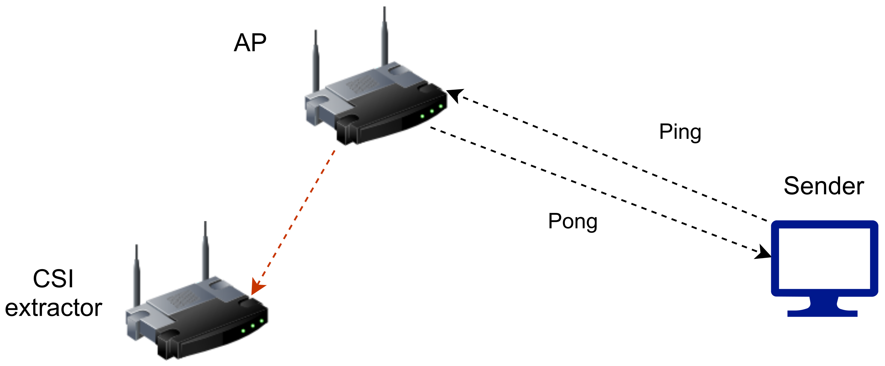
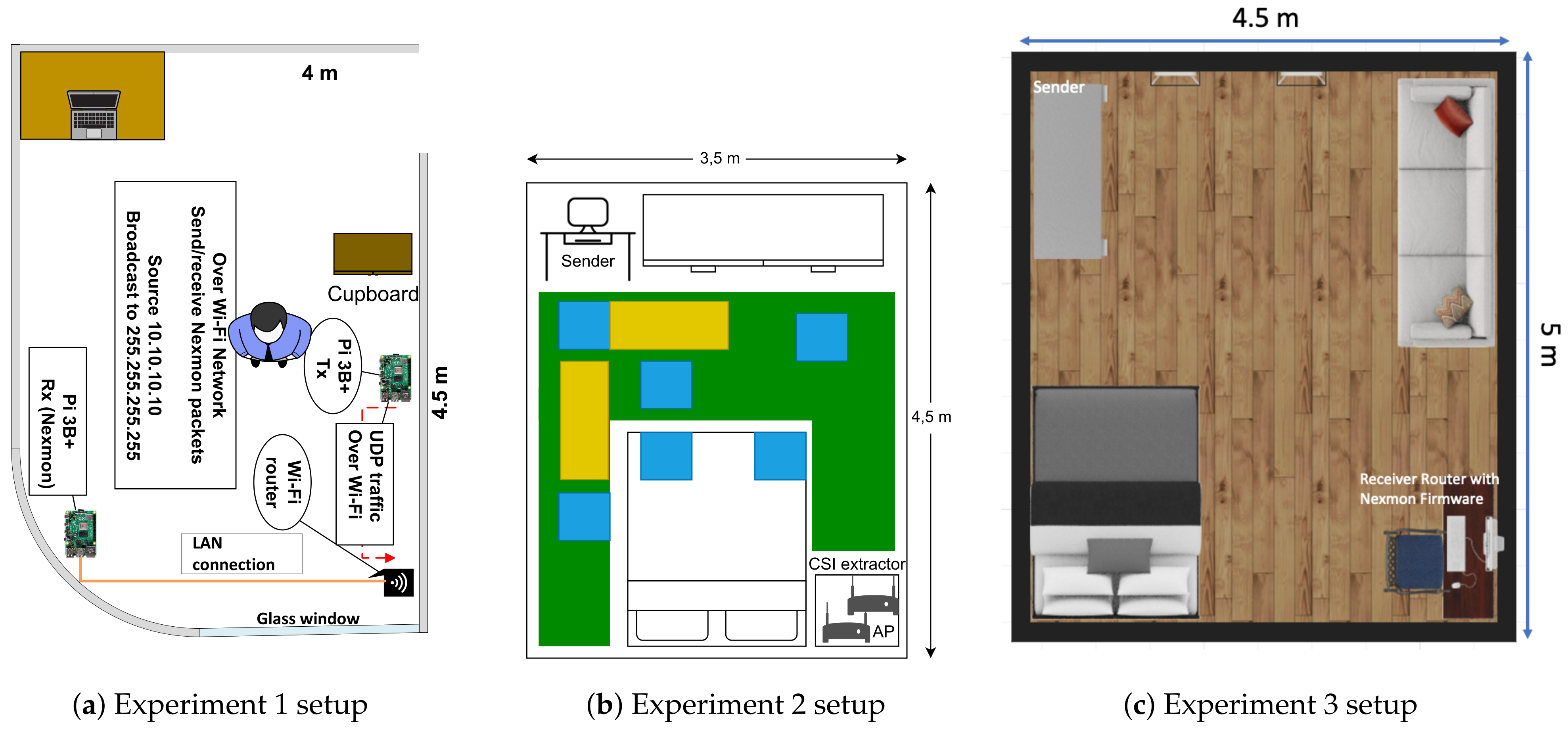
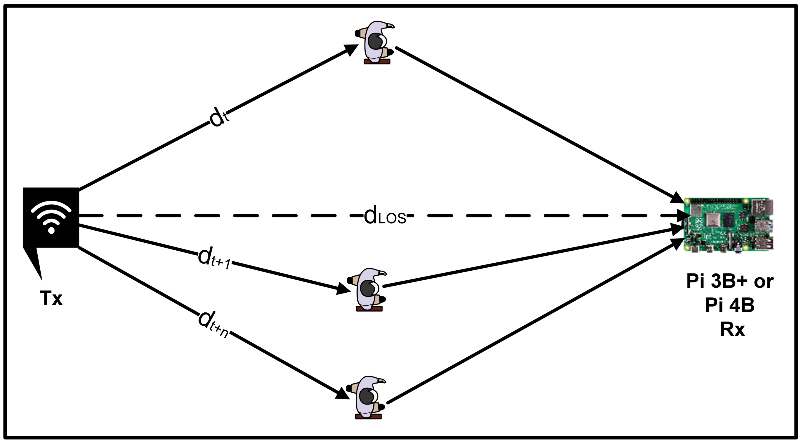


