Online Efficiency Optimization and Speed Sensorless Control of Single-Phase Induction Motors

Abstract

Single phase induction motors (SPIM) are widely used in residential and commercial applications. Enhancement of efficiency of SPIMs can lead to huge energy savings. This paper presents a novel mechanical sensorless control method for SPIM drives. In this method, a machine learning algorithm is used to estimate the slip based on the ratio of main and auxiliary winding currents. To enhance the efficiency, the terminal voltage is reduced under light load conditions. The optimal operating voltage is implicitly obtained by equating the ratio of main and auxiliary winding currents to its optimum value. This optimal operating point is first calculated based on the frequency from a lookup table and then updated by using gradient descent algorithm. This way, the optimal operating point is realized despite motor parameter variations. The proposed scheme is suitable for low-power applications where working at different speeds and load torques is demanded, such as ventilation systems and various household appliances. Simulation results are presented to verify the efficacy of the proposed method.

1. Introduction

The increasing of electricity prices and the public awareness of environmental problems associated with conventional power plants motivate major attention in enhancing the efficiency of electrical devices. Numerous domestic, commercial and some light-duty industrial applications, near which there is no easy access to three-phase networks, utilize single-phase induction motors (SPIMs). SPIMs have the advantages of low cost and high reliability. However, they have a relatively low efficiency compared with alternative solutions such as permanent magnet synchronous motors. As such, the amount of power loss caused by SPIMs is significant. Therefore, enhancing the efficiency of SPIMs can have a major impact on the overall power losses of electrical systems.

An SPIM is comprised of two stator windings (i.e., main and auxiliary winding) and a squirrel cage rotor. The two windings, which are in space quadrature, usually have different impedances. A phase shifting capacitor is placed in series with the auxiliary winding to produce an appropriate phase shift in the auxiliary winding current. The combination of auxiliary winding and the capacitor is paralleled with the main winding, which is connected to the motor terminals. The SPIM can be directly connected to the electrical grid. To control the speed and optimize its efficiency, a variable speed electric motor drive can be employed, in which a power electronic converter is connected between the SPIM and the grid. Figure 1 depicts the schematic of the SPIM drive, in which a Single-Phase Bridge Inverter is used to control a capacitor-run SPIM. The AC line voltage is rectified and filtered via a diode-bridge and a capacitor, and is fed to the Inverter. The amplitude and frequency of the sinusoidal reference is governed by the controller.

A number of methods are proposed for speed control of induction motors, including rotor-flux-oriented control [1,2], vector control [3], direct torque control [4,5], sliding mode control [6], neural network based control methods [7,8] and a model predictive control method [9]. Furthermore, various speed sensorless control methods have been proposed, among them are a method based on DC-link measurements [10], speed measurement based on rotor-slot-related harmonic detection in machine line current [11], field-orientation control with a speed estimation scheme [11] and speed estimation using adaptive nonlinear observers [12] and sliding mode observer [13]. The mentioned control schemes, which are focused on the speed control dynamics, do not take action for optimization of the efficiency.

The efficiency of induction motors can be enhanced by adjusting the applied voltage and hence the flux at the optimum operating point [14]. In order to obtain the optimum operating point corresponding with each speed and load, one can use the loss model of the motor [15,16]. In [17] the dynamic model of induction machine has been used to derive an algorithm for calculating the optimum flux. However, the aforementioned approaches require the exact value of the motor parameters through a parameter identification scheme [18]. A real time efficiency optimization method has been presented in [19]. In this method, the optimal flux is first calculated analytically based on the estimated motor parameters and then updated in real time using annealing method. The methods of [15,16,17,18,19] are focused on three-phase induction motors. Reference [20] proposes a control scheme for enabling symmetrical and balanced operation of SPIM during both starting and steady-state operating conditions. Although such symmetrical operation enhances the efficiency, the requirement of two full bridge converters for main and auxiliary windings increases the cost of the system. In a method presented in [21] the ratio of main to auxiliary stator winding currents (Stator Current Ratio) is used as the optimization parameter. It is shown that controlling this parameter can lead us to the optimum operating condition, regardless of the motor speed and torque. Hence, an efficiency optimization method with no mechanical sensor requirements was attained. This method has been further developed with varying frequency in [22], which utilizes the phase difference of main and auxiliary stator winding currents. Although this method might be appealing to SPIM drives due to the rather cheap and simple implementations, major deficiencies lie within it. Firstly, it lacks any sort of speed regulation due to its open loop speed control scheme. In addition, it is sensitive to motor parameters variations. In some of the proposed methods the optimum operating point of the motor is determined via utilizing machine learning approach [23]. The aforementioned method requires mechanical sensors for the aim of measurements, which make them rather impractical and uneconomical for the case of SPIMS.

The motor parameters are prone to change due to environmental conditions, temperature variations, saturation and discrepancy of the same model motor parameters. These changes lead to deflection in the optimal efficiency point [24]. Therefore, in case of applying the methods which are offline, the controller would naturally be unable to track the deflected optimal efficiency point and henceforth the motor efficiency would never be the ultimate maximum. Furthermore, parameter variations can degrade the accuracy of speed estimation algorithms [12]. To deal with this issue, this paper proposes a novel speed sensorless and optimal efficiency control method for SPIMs. In the proposed method, the motor speed is estimated based on Stator Current Ratio using a neural network. Furthermore, the optimum efficiency conditions are derived using an online loss minimization method. This way, in addition to tracking the optimum operating point in online mode, accurate speed regulation is realized. The proposed method is verified by running a simulation using MATLAB software.

The rest of the paper is organized as follows. The mathematical model of SPIM is addressed in Section 2. Speed estimation and efficiency optimization methods are explained in Section 3 and Section 4, respectively. The proposed control scheme is addressed in Section 5. Simulation results are addressed in Section 6. Section 7 concludes the paper.

2. Mathematical Model of SPIM

2.1. Stator Current Ratio

According to [21] the ratio of main to auxiliary stator windings currents (STCR) is expressed as:

$$Z_t=\frac{I_m}{I_a}=\frac{2Z_{1a}+a^2\left(Z_f+Z_b\right)+ja\left(Z_f-Z_b\right)}{2Z_{1m}+Z_f+Z_b-ja\left(Z_f-Z_b\right)}$$

(1)

where a is the turns ratio of auxiliary to main winding, Z_1a, Z_1m, Z_f, and Z_b are defined in terms of slip (s), synchronous frequency (ω_e), auxiliary winding capacitance C, and machine inductances, as follows [21]:

$$Z_f=\frac{-s{L}_{ms}{L}_{lr}^{\prime }{\omega }_e^2+j{R}_r^{\prime }{L}_{ms}{\omega }_e}{R_r^{\prime }+js{\omega }_e\left(L_{ms}+L_{lr}^{\prime }\right)}$$

(2)

$$Z_b=\frac{-(2-s)L_{ms}{L}_{lr}^{\prime }{\omega }_e^2+j{R}_r^{\prime }{L}_{ms}{\omega }_e}{R_r^{\prime }+j(2-s){\omega }_e\left(L_{ms}+L_{lr}^{\prime }\right)}$$

(3)

$$Z_{1m}=R_{sm}+j{L}_{lsm}{\omega }_e$$

(4)

$$Z_{1a}=R_{sa}+j\left(L_{lsa}{\omega }_e-\frac{1}{C{\omega }_e}\right)$$

(5)

2.2. Electrical Torque

Single-phase induction motor torque is expressed as [21]:

$$T_e=\frac{2}{{\omega }_e}\left(I_{mf}^2{R}_f-I_{mb}^2{R}_b\right)$$

(6)

where $R_f=\mathrm{Re}\{Z_f\}$ and $R_b=\mathrm{Re}\{Z_b\}$. Equation (6) can be expressed in terms of I_m as follows:

$$T_e=\frac{1}{2{\omega }_e}{I}_m^2\left(R_f{\left|1-j\frac{a}{Z_t}\right|}^2-R_b{\left|1+j\frac{a}{Z_t}\right|}^2\right)=I_m^2{A}_1$$

(7)

Since Z_t is a function of motor parameters, namely supply frequency (ω_e) and motor slip (s) therefore we have:

$$A_1=f\left({\omega }_e,s\right)$$

(8)

2.3. Power Losses in SPIM

The electrical losses of SPIM are as follow:

• Stator copper losses. Copper losses in the main and auxiliary stator windings are given by [21]:

  $$P_{cus}=I_m^2{R}_{sm}+I_a^2{R}_{{}_{sa}}$$

  (9)

  Substituting the auxiliary winding current in the right-hand side of (9) with the expression $I_m/Z_t$ (as per (1)), the stator copper losses can be expressed as:

  $$P_{cu}=I_m^2\left(R_{sm}+\frac{R_{sa}}{{\left|Z_t\right|}^{{}^2}}\right)$$

  (10)
• Rotor copper losses. Copper losses in the rotor winding can be written as:

  $$P_{cur}=I_r^{\prime }{}^2{R}_r^{\prime }=I_m^2{R}_r^{\prime }{\left|\frac{1-j\frac{a}{Z_t}}{\frac{R_r^{\prime }}{s}+j{L}_{lr}^{\prime }{\omega }_e}+\frac{1-j\frac{a}{Z_t}}{\frac{R_r^{\prime }}{2-s}+j{L}_{lr}^{\prime }{\omega }_e}\right|}^{{}^2}$$

  (11)
• Core losses. Core losses which include hysteresis and eddy current losses are given by [21]:

  $$P_{fe}=c_{fe}\left(E_{mf}^2+E_{mb}^2\right)$$

  (12)

Then, the aforementioned equation can be expressed in terms of I_m as follows:

$$P_{fe}=\frac{c_{fe}}{4}\left({\left|Z_f\right|}^2{\left|1-j\frac{a}{Z_t}\right|}^2+{\left|Z_b\right|}^2{\left|1+j\frac{a}{Z_t}\right|}^2\right)I_m^2$$

(13)

4.

Stray load losses: Stray load losses are due to changes made in the flux distribution and eddy currents given by the following empirical expression:

$$P_{str}=c_{str}{I}_r^{\prime }{}^2{\omega }_e^2$$

(14)

It can further be expressed in terms of I_m:

$$P_{str}=c_{str}{I}_m^2{\omega }_e^2{\left|\frac{1-j\frac{a}{Z_t}}{\frac{R_r^{\prime }}{s}+j{L}_{lr}^{\prime }{\omega }_e}+\frac{1-j\frac{a}{Z_t}}{\frac{R_r^{\prime }}{2-s}+j{L}_{lr}^{\prime }{\omega }_e}\right|}^{{}^2}$$

(15)

By summing all the losses expressions in terms of I_m and factoring, it yields:

$$P_{el}=I_m^2{A}_2$$

(16)

In this equation, A₂ is a variable being function of motor parameters, the applied frequency and slip, written as:

$$A_2=g\left({\omega }_e,s\right)$$

(17)

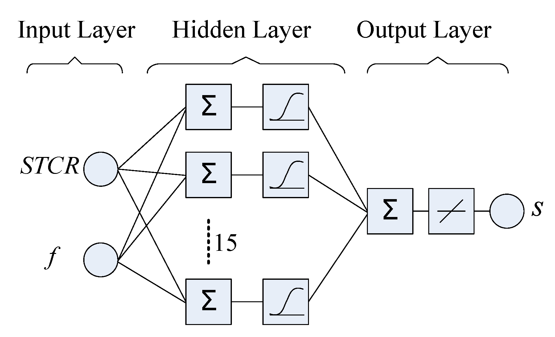
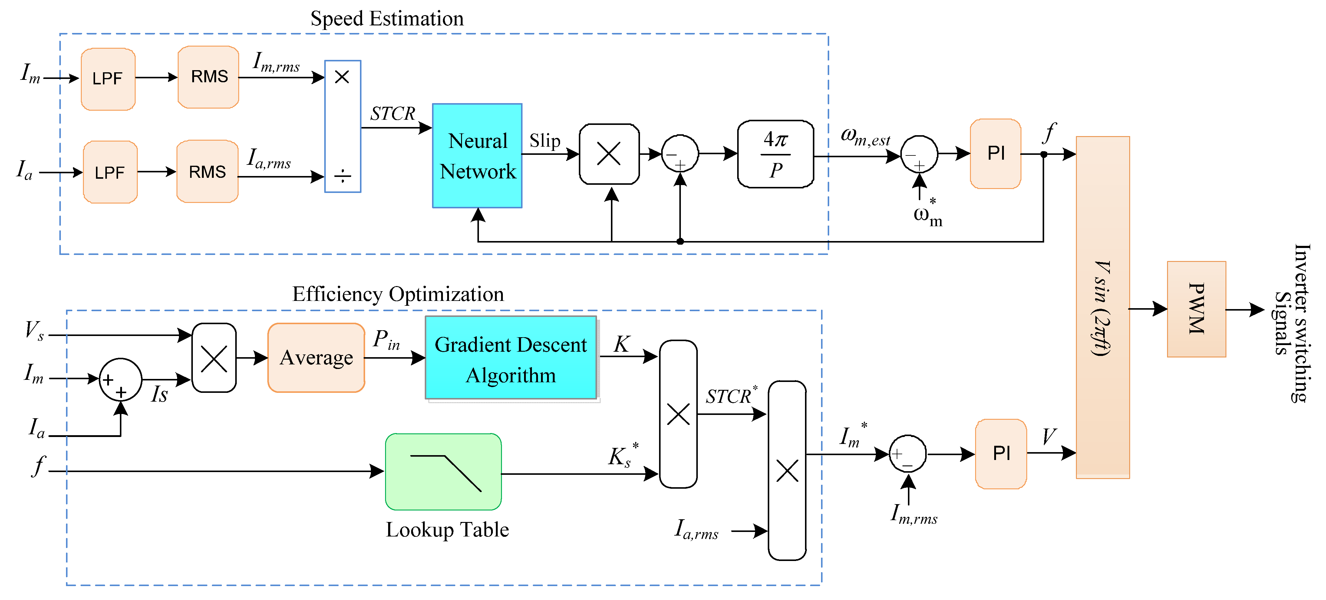
3. Sensorless Speed Estimation

By substituting (2)–(5) into (1), STCR can be expressed as a function of supply frequency (ω_e), slip (s) and the motor parameters. Assuming the motor parameters are fixed, SCTR can be expressed in the following fractional form:

$$Z_t=\frac{I_m}{I_a}=\frac{N({\omega }_e,s)}{D({\omega }_e,s)}$$

(18)

where N, D are complex polynomials, which are all functions of s and ω_e. By taking the absolute value of both sides of (18) and rearranging, the following equation can be driven:

$$\left|D({\omega }_e,s)\right|\left|Z_t\right|-\left|N({\omega }_e,s)\right|=0$$

(19)

At every operating point, $\left|Z_t\right|=\left|I_m\right|/\left|I_a\right|$ can be calculated from measured rms values of the main and auxiliary winding currents. Since the applied frequency (ω_e) is known, slip can be calculated by solving (19). For an expeditious and accurate response, a Neural Network (NN) has been employed.

The NN utilized, which is shown schematically in Figure 2, is a feedforward network with one hidden layer. It consists of two inputs (STCR and frequency f) in the input layer, 15 neurons in the hidden layer and only one output (estimated slip) at the output layer. To train the NN more accurately, numerous sample data are required. To do so, the STCR will be calculated for 100 values of slip at 16 different frequencies using (1) as shown in Figure 3. Then, entering f and the calculated STCR as inputs of NN and assigning the corresponding slips as the expected output (targets), the NN will be ready for training.

The back-propagation Levenberg-Marquardt training method in batch mode is used, which appears to be the fastest method for training moderate-sized feedforward neural networks with the great ability of avoiding the local minima. The learning rate (l_r) is set to as low as 0.005, since the number of sample training data is relatively large, and an unwisely large learning rate would lead to divergence of the training algorithm. The number of iterations (epochs) is set to 1000. The train goal, which is the trained network total accumulative error to be met by the algorithm, is set to 10⁻⁸.

Having attained the slip from the output of the trained neural network, the motor speed can be calculated via following equation:

$${\omega }_m=(1-s)\times \frac{2}{P}\times {\omega }_e$$

(20)

The obtained motor speed will further be used as the motor speed feedback and will be applied to the speed control loop. Hence, we are able to have speed regularization without any speed sensors being used. The speed estimation error (${\omega }_{m,error}$) is defined as follows:

$${\omega }_{m,error}=\frac{{\omega }_{m,est}-{\omega }_m}{{\omega }_m}$$

(21)

The speed estimation error serves as a performance index of the speed estimator module and will be monitored throughout the simulation.

4. Energy Efficiency Optimization

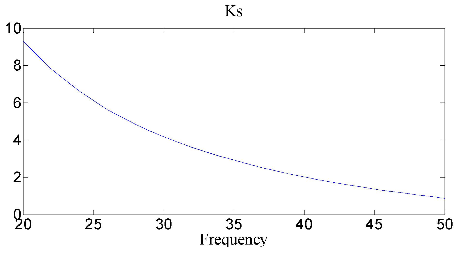
4.1. Optimal Energy Efficiency Condition

When the mechanical load is decreased away from its nominal value, the motor efficiency will drop. This stems from the fact that since the reactive part of the current does not decline with the load decrease, the load decrease hence is not proportional to the current and copper loss decrease. Further, the core loss which is proportional to the applied voltage will not change at all. Therefore, the motor loss in light loads would not change considerably. Given the output decrease and the rather constant loss, the efficiency will drop. On the other hand, by decreasing the input voltage the core loss will drop substantially with square of the voltage, while the copper loss by an increase in the active part of the current begins to increase slightly. This voltage decrease should be in a controlled manner to a voltage point where the total loss is minimum. It is apparent that decreasing the voltage only down to a certain value causes the total loss to decrease and efficiency to increase, after which the motor loss will start to increase [21].

The motor-developed torque is equal to the load torque plus windage and mechanical losses, which are all constant at state conditions. As such, the developed torque is also constant and its derivate is zero [21]:

$$\frac{\partial T_e}{\partial s}=0$$

(22)

According to (7), the following equation will be obtained:

$$2A_1{I}_m\frac{\partial I_m}{\partial s}+I_m^2\frac{\partial A_1}{\partial s}=0$$

(23)

The optimum slip (s_opt) is the slip of the operating point at which the loss is at minimum. Assuming that the machine torque and supply frequency are constant (motor is operating at steady-state condition), the optimum slip can be calculated by setting the derivative of electrical losses with respect to slip to zero:

$${\frac{\partial P_{el}}{\partial s}|}_{T_e,{\omega }_e}=0$$

(24)

Using (16), condition (24) is satisfied when

$$2A_2{I}_m\frac{\partial I_m}{\partial s}+I_m^2\frac{\partial A_2}{\partial s}=0$$

(25)

From (23), (25), by eliminating I_m yields:

$$\frac{1}{A_1}\frac{\partial A_1}{\partial s}-\frac{1}{A_2}\frac{\partial A_2}{\partial s}=0$$

(26)

Since at every operating point, the supply frequency is constant, A₁ and A₂ are only dependent upon slip variations. Hence, from the above equation the optimum slip is attainable.

Substituting s_opt into (1) the optimum STCR can be introduced as follows:

$${\left(\frac{I_m}{I_a}\right)}_{opt}={\left|Z_t\right|}_{s=sopt}=K_s$$

(27)

where, according to (1), K_s is only a function of frequency and motor parameters.

In case of neglecting motor parameters slight variations, the optimum STCR (K_s) would only be dependent upon the supply frequency.

$$K_s=h\left({\omega }_e\right)$$

(28)

To obtain K_s, the motor is supplied with a variable frequency and amplitude AC source. Keeping the frequency and mechanical load constant, the voltage amplitude is varied between 20% to 100% of the nominal value and then the input power, stator main and auxiliary winding currents are measured. Further, STCR will be determined by dividing the two windings’ currents. After drawing a diagram of input power (P_in) versus STCR, the minimum value of input power and its corresponding STCR value will be determined. As such, the optimum STCR (K_s) is determined. Repeating the same procedure for different frequencies, the K_s for each frequency will be obtained. Further the frequency and its corresponding K_s pairs will be saved in a table as a lookup table in the controller’s memory and will be used as the reference value of K_s.

Hence, the optimum condition will be achieved for constant pre-known motor parameters. Nevertheless, factors such as saturation and temperature variations will cause changes in some of the motor parameters such as resistances and inductances. In addition, it cannot be expected that all of a factory’s same-model motors will have the exact same parameter values. Therefore, calculating a unique optimum point seems to be unattainable.

4.2. Gradient Descent Algorithm

In order to minimize the SPIM loss, taking into account motor parameters variations, the corrective parameter K is defined to update K_s. K is calculated online using an optimization algorithm called Gradient Descent [25]. The algorithm is described as follows:

• The initial value of K is set to 1, which is the case where no correction is yet made to K_s. The input power (P_in) is measured for this case. Then, the initial value of K variation ($\Delta \mathit{K}$) is set to an arbitrary value, the iteration index (i) is set to 1, the convergence criterion is ε and the convergence factor is $\lambda$.
• The values of K are updated via following equation:

  $$K^{(i+1)}=K^{(i)}+\mathsf{\Delta }K$$

  (29)
• After a specified time, which takes into account the time required before the changes made in K_s appear in the motor operation and motor reaches to a new stable state, the new input power (P_in) is measured.
• Inasmuch as after passing through the transient state, the motor speed will be regulated and reaches its set value; the load power, therefore will be equal to its previous value. As a result, changes in input power will be equal to changes in loss. Therefore, the algorithm is expected to work equally by using the input power instead.
  In other words:

  $$P_{in}^{(i+1)}-P_{in}^{(i)}=[P_{out}^{(i+1)}+P_{loss}^{(i+1)}]-[P_{out}^{(i)}+P_{loss}^{(i)}]=P_{loss}^{(i+1)}-P_{loss}^{(i)}$$

  (30)

It is important to note that for a reliable performance of the optimization module, the time delay between consecutive iterations shall be long enough to let the speed transients diminish adequately.

5.

The approximated power loss gradient is calculated as follows:

$$\nabla P_{loss}=\frac{d{p}_{loss}}{dk}\cong \frac{\mathsf{\Delta }{P}_{loss}}{\mathsf{\Delta }K}=\frac{P_{in}^{(i+1)}-P_{in}^{(in)}}{K^{(i+1)}-K^{(i)}}$$

(31)

6.

In order to approach the minimum point of power loss, K must change in the opposite direction of power loss gradient i.e.,

$$\mathsf{\Delta }K=-\lambda \nabla P_{loss}$$

(32)

7.

If ΔK is smaller than ε, the algorithm will be stopped. Otherwise, the iteration index (i) is increased by one and the algorithm will return to step 2.

It is noteworthy that this algorithm has a deficiency of getting trapped in local minima. In our case, however, as there is only one minimum to be found [21], such deficiency is dismissed.

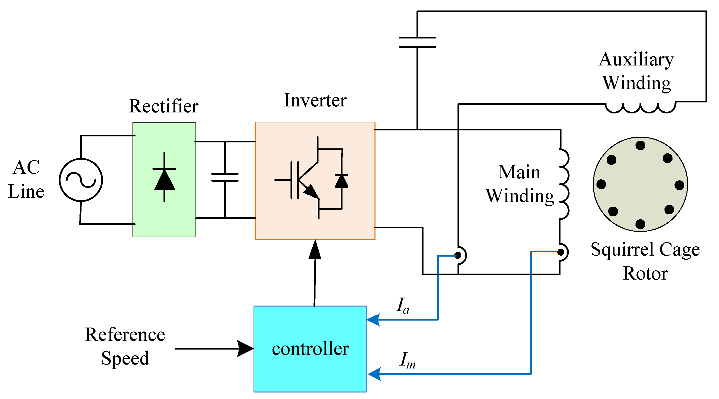
5. Control Scheme Implementation

The controller consists of two main parts of frequency and voltage control. Figure 4 illustrates the block diagram of the controller. This system, which is void of any mechanical sensors, utilizes STCR for motor speed estimation. For this purpose, the main and auxiliary winding currents are measured via current sensors. After removing noise and high frequency components using a Low Pass Filter (LPF), the rms values are calculated and later, by dividing the rms values of main and auxiliary winding currents, the STCR will be obtained.

As previously stated in Section 3, the NN estimates the motor slip utilizing STCR and frequency. The evaluated slip is further used to calculate the speed (ω_m,est), which acts like a mechanical speed sensor and is used as the speed feedback to the motor speed controller. The speed controller consists of a PI controller commanding the reference frequency of inverter.

In addition to speed control, the presented system is capable of optimizing the motor efficiency. To carry out this, the motor voltage should be adopted according to the value commanded by the voltage controller. The voltage controller maximizes the efficiency by adapting the input voltage amplitude. To do so, K_s^* is initially extracted from the lookup table according to the set frequency and further multiplied by the corrective factor (K), which is determined by the optimization module, to give the final optimal value of STCR. The voltage controller later attempts to drive the STCR to its optimal designated value through reducing the voltage amplitude. In this process, firstly the optimum value of stator main winding current (I_m^*) is calculated via multiplying the optimal SCTR by the measured auxiliary winding current. A closed-loop PI controller regulates the main winding current to its reference value (I_m^*). The time constant of this controller is larger compared to that of speed controller in such a way that the voltage amplitude variations have almost no bearing on the frequency transients. The optimization algorithm requires the power loss measurement. However, as it is not practical to measure the power loss directly, the input power is used instead, as previously described in Section 4.

In spite of providing the two objectives of speed regulation and efficiency optimization, the drive utilizes merely two current sensors as feedbacks. The control algorithm is rather simple and does not demand a fast-processing technology for implementation. Therefore, the controller and SPWM signal generator can both be implemented in an inexpensive microcontroller. The controller’s simplicity, on the one hand, and speed sensor-free feature, on the other hand, makes the proposed drive quite suitable for low-power and less expensive applications.

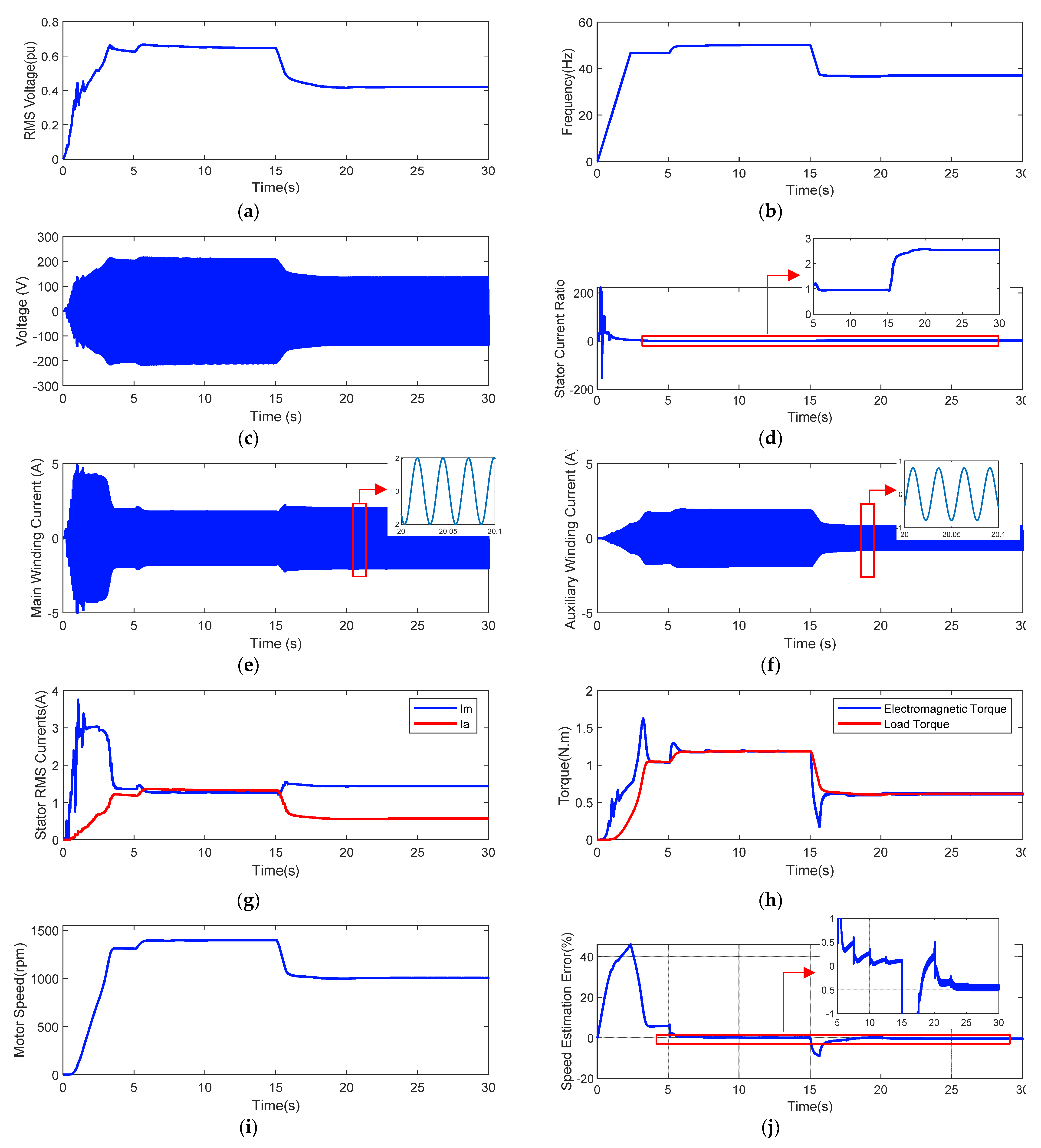
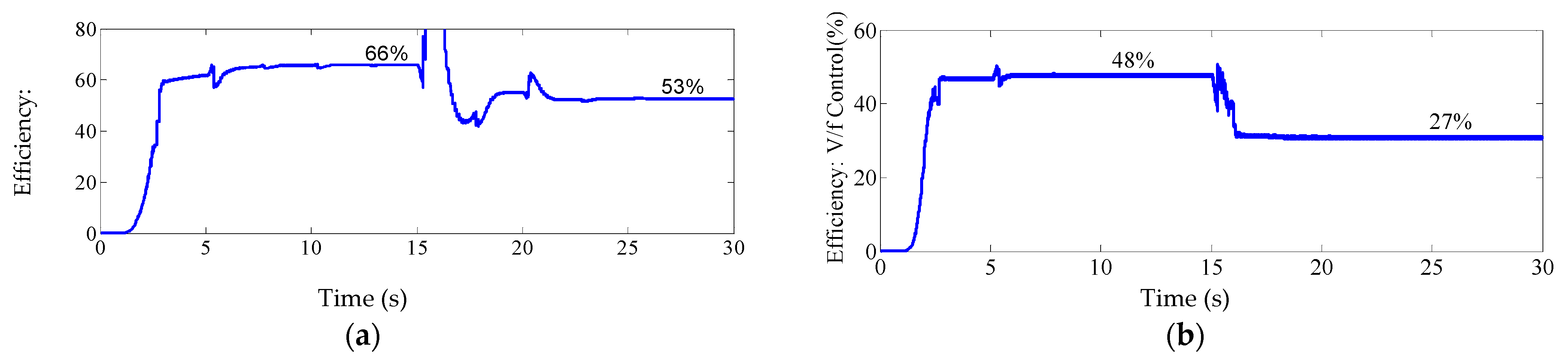
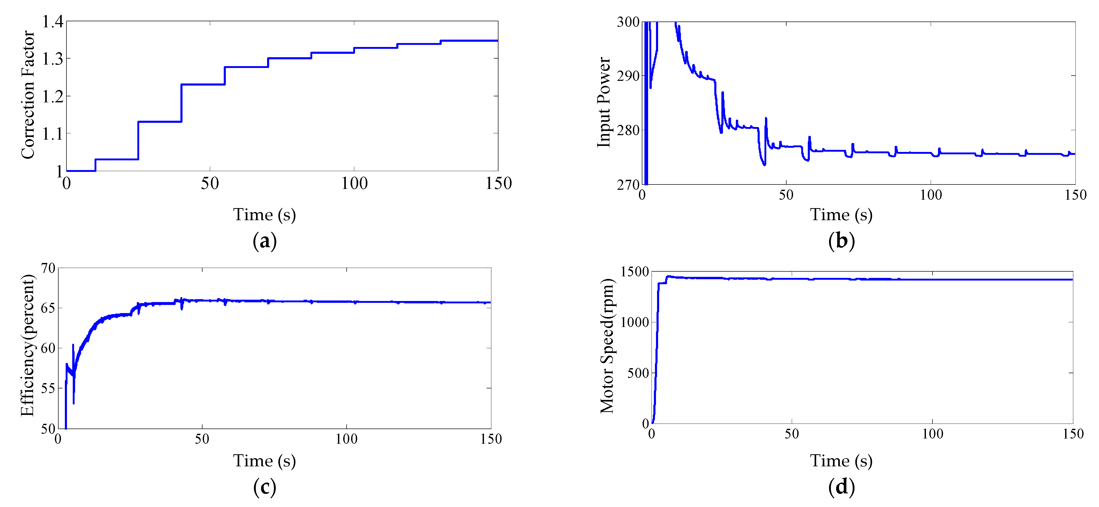
6. Simulation Results

The presented control scheme is simulated in MATLAB software to verify its performance. A four-pole 0.5 horsepower capacitor-run SPIM is employed, the characteristics of which are listed in

Table 1. Motor parameters.

Parameter		Value	Unit
Nominal Values	Voltage	220	V
	Frequency	50	Hz
	Power	0.5 × 746	W
	Speed	1440	rpm
	Load Torque	2.4	N·m
Main Winding Stator	Resistance	15	Ω
	Leakage Inductance	40	mH
Main Winding Rotor	Resistance	12.1	Ω
	Leakage Inductance	48.4	mH
Auxiliary Winding Stator	Resistance	16.5	Ω
	Leakage Inductance	48.4	mH
	Series capacitance	18	μF
Main Mutual Inductance		350	mH
Turns ratio of auxiliary to main winding		1.1	-
Inertia		0.01	Kg·m2
Iron Loss Equivalent Resistance		1000	Ω

. Other simulation parameters such as PI controller coefficients and motor reference speed are listed in

Table 2. Controller parameters.

Parameter		Value
PI frequency controller	Proportional Coefficient, Kp	9 × 10−4
	Integrator Coefficient, Ki	5
PI voltage controller	Proportional Coefficient, Kp	0.108
	Integrator Coefficient, Ki	0.862
Gradient descent algorithm	Time Delay	5 s
	convergence criteria (ε)	0.1
	convergence coefficient (λ)	0.01
	Initial value of corrective factor variation (ΔK)	0.05
Neural network	Sample Time	0.01 s

.

Using a variable-amplitude voltage source, K_s is calculated for different frequencies varying between 20 to 50 Hz, as described in chapter IV. Figure 5 depicts the diagram of K_s versus frequency. This diagram is saved as a lookup table and is used as a reference for the controller.

The performance of the proposed drive is verified through three simulation scenarios. In the first scenario, the motor is initially at standstill. The reference speed is set to 1440 rpm and the load, which is of fan type, is set to 50% nominal. The motor starts at t = 0. Then, at t = 15 s, the reference speed is changed from nominal to 1000 rpm. As shown in Figure 6a–c, the controller’s output voltage and frequency increase with a limited rate to realize a soft start. After the starting period, the speed control loop adjusts the frequency at 51.5 Hz to regulate the motor speed at its set point (1440 rpm) and controls the voltage magnitude at 0.65 pu to ensure the stator current ratio settles at the optimal value of 0.96 (see Figure 6d,i). The waveforms of the instantaneous and rms stator currents are shown in Figure 6e–g. It is seen that during the starting phase, the main winding current is higher than the auxiliary winding current. This behavior is mainly caused by the fact that the voltage to frequency ratio at the starting phase is set to unity. Afterwards, the main winding current drops to below the auxiliary winding current due to the reduction in v/f ratio. It is noteworthy to highlight that the reduction in v/f ratio and hence the flux is the key to enhancing the efficiency at light loading conditions. As shown in Figure 6h, the electromagnetic torque is higher than the load torque during the starting phase, when the motor accelerates. Since the mechanical and windage losses are omitted, both motor and load torque settle at 1.2 Nm (50% of nominal) at steady-state. The speed estimation error is initially large but reduces to as low as 0.5% in the steady state, providing decent speed regulation.

At t = 15 s, the reference speed is reduced to 1000 rpm. In order to track the new speed set point, the frequency is decreased to 37 Hz (see Figure 6b). Furthermore, as shown in Figure 6a,d, the STCR is changed to the new optimum value (2.5) by reducing the voltage magnitude to 0.41 pu. As shown in Figure 6e–g, as the STCR increases at t = 15 s, the main winding current slightly increases whereas the auxiliary winding current experiences a significant drop. Since the mechanical load is a fan, its torque is proportional to the square of speed. As such, when the speed drops from 1440 rpm to 1000 rpm, the load torque halves, as shown in Figure 6h. Furthermore, the electromagnetic torque dips below the load torque during transients to provide deceleration but then settles at the same value.

The efficiency of the proposed drive is compared with a constant-v/f based drive in Figure 7. It can be seen that the proposed drive makes an improvement of 18% in the motor efficiency at a 50% load. Comparing the efficiency of the proposed drive with constant-v/f based drive, a 26% improvement is witnessed, which is a better improvement than the previous case, and is majorly due to the reduction in load torque.

In the second scenario, the drive’s performance to a load disturbance of 50% while speed set point is fixed at 1440 rpm is evaluated. Figure 8 show the simulation results of the second scenario. The load torque is initially at 50% of nominal, namely 1.2 N·m. The load torque is increased from 1.2 N·m to 2.4 N·m at t = 20 s and then changed back to 1.2 N·m at t = 35 s (see Figure 8h). Following this, the controller output voltage (shown in Figure 8a) is increased to provide the nominal torque while maintaining STCR fixed at the optimal value of 0.96. Moreover, the frequency is slightly increased to retain the motor speed at its reference value (see Figure 8b). As shown in Figure 8e–g, the main winding current increases above the auxiliary winding current during the transient acceleration period but then drops such that STCR becomes equal to 0.96. As depicted in Figure 8i, the motor speed experiences slight undershoot during the load rise but settles at it set point after a few seconds. The speed estimation error steps up to 12% at first, though diminishes to 1% after 2 s. The efficiency of constant-v/f based drive changes from 43% to 63%, while the efficiency of the proposed drive is constant and equal to 66% in both half and full load conditions, as shown in Figure 9.

In the third scenario, in order to demonstrate the efficacy of the control scheme in tracking the optimum condition, notwithstanding the motor parameters variations, the motor parameters are to be changed. Given a specific frequency, for each set of motor parameters there exists a unique K_s. Therefore, when parameters change, K_s must be updated. As it is both impractical and unnecessary to model all factors accurately, the motor parameters are subjected to a random change up to 10% taking into account all the parameter variation factors. Then, it is observed that, as expected, the K_s outputted by the look-up table is gradually updated to the optimum STCR, which can be known as the K_s for the new motor parameters.

Figure 10 depicts the correction factor (K), the input power, efficiency and motor speed variations during the simulation. From Figure 10a, it can be seen that during the iterations of optimization, each of which lasts for 15 s, K is making step changes towards the optimum point and after some time finally reaches a fixed value (1.33). After changing the value of K in each iteration, the input power passes through transient fluctuations and reaches a stable point (see Figure 10b). By observing these stable points, a decreasing trend is seen, which finally decays to a fixed stable operating point. As shown in Figure 10c, the efficiency moves in an increasing trend towards a fixed optimal efficiency, which equals 66%, while the efficiency of the motor without optimization control for the same load (50% nominal), is seen to be as low as 48% (see Figure 9b). Therefore, the efficiency improvement for this case is 18%, which declines as the load increases toward the nominal value. The motor speed is regulated to the reference value of 1440 rpm throughout the optimization process, which means that changes enforced by the optimization module are not creating any disturbances that may possibly lead to maloperation of the motor.

7. Conclusions

In this paper, a novel single-phase inverter-based drive has been proposed to provide us with speed control and optimum efficiency for SPIMs. Since SPIMs are a low rating and rather inexpensive kind of motor, being affordable and mechanical sensor-free were introduced as the major issues to be addressed. To realize closed loop speed control without using mechanical sensors, a new speed estimation technique has been addressed. This method is developed based on the fact that STCR is dependent on the slip and operating frequency. Accordingly, the slip is estimated based on the known operating frequency and measured value of STCR using a NN. The estimated slip is then used to obtain the rotor speed, which is fed to the speed controller which determines the reference frequency. To minimize the motor losses, the voltage magnitude is adjusted based on an online efficiency optimization method. In this method, the optimum operating voltage is indirectly calculated by using a PI controller which attempts to realize the optimum SCTR. The advantage of this strategy is that unlike optimal voltage, the optimum SCTR is independent of the load but only depends on the frequency and motor parameters. The optimum SCTR is first calculated based on the operating frequency from a lookup table (offline) and then updated using gradient decent algorithm (online). The foremost advantage of the proposed online optimization method comparing to the preceding methods is its independency upon motor parameters. The proposed control strategy has been verified by simulation results. The simulation results show that the proposed control scheme provides a considerable enhancement in term of energy efficiency while realizing speed regulation. Although the closed loop system does not provide fast dynamics, this limitation is not considered to be a major issue for the intended applications (ventilation systems and house appliances).

The future work following this paper would include implementation of the drive and then commercializing it. The simplicity of the controller, being mechanical sensor-free and its independency on a specific motor make the proposed drive potentially marketable.

References

1. De Correa, M.B.R.; Jacobina, C.B.; Lima, A.M.N.; de Silva, E.R.C. Rotor-flux-oriented control of a single-phase induction motor drive. IEEE Trans. Ind. Electron. 2000, 47, 832–841. [Google Scholar] [CrossRef]
2. Arpit, G.; Singh, H.P.; Pandey, K. Advance speed control of three phase induction motor using field oriented control method. Mater. Today Proc. 2021. [Google Scholar] [CrossRef]
3. Akhtar, M.J.; Behera, R.K. Space Vector Modulation for Distributed Inverter-Fed Induction Motor Drive for Electric Vehicle Application. IEEE J. Emerg. Sel. Top. Power Electron. 2021, 9, 379–389. [Google Scholar] [CrossRef]
4. Aktas, M.; Awaili, K.; Ehsani, M.; Arisoy, A. Direct torque control versus indirect field-oriented control of induction motors for electric vehicle applications. Eng. Sci. Technol. Int. J. 2020, 23, 1134–1143. [Google Scholar] [CrossRef]
5. El Ouanjli, N.; Derouich, A.; El Ghzizal, A.; Motahhir, S.; Chebabhi, A.; El Mourabit, Y.; Taoussi, M. Modern improvement techniques of direct torque control for induction motor drives—A review. Prot. Control. Mod. Power Syst. 2019, 4, 11. [Google Scholar] [CrossRef] [Green Version]
6. Dòria-Cerezo, A.; Olm, J.M.; Repecho, V.; Biel, D. Complex-valued sliding mode control of an induction motor. IFAC-Pap. 2020, 53, 5473–5478. [Google Scholar] [CrossRef]
7. Fu, X.; Li, S. A Novel Neural Network Vector Control Technique for Induction Motor Drive. IEEE Trans. Energy Convers. 2015, 30, 1428–1437. [Google Scholar] [CrossRef]
8. Quintero-Manríquez, E.; Sanchez, E.N.; Antonio-Toledo, M.E.; Muñoz, F. Neural control of an induction motor with regenerative braking as electric vehicle architecture. Eng. Appl. Artif. Intell. 2021, 104, 104275. [Google Scholar] [CrossRef]
9. Sahu, A.; Mohanty, K.B.; Mishra, R.N. Development and experimental realization of an adaptive neural-based discrete model predictive direct torque and flux controller for induction motor drive. Appl. Soft Comput. 2021, 108, 107418. [Google Scholar] [CrossRef]
10. Sonnaillon, M.O.; Bisheimer, G.; de Angelo, C.; Solsona, J.; Garcia, G. Mechanical-sensorless induction motor drive based only on DC-link measurements. IEE Proc.-Electr. Power Appl. 2006, 153, 815–822. [Google Scholar] [CrossRef]
11. Nandi, S.; Ahmed, S.; Toliyat, H.A.; Bharadwaj, R.M. Selection criteria of induction machines for speed-sensorless drive applications. IEEE Trans. Ind. Appl. 2003, 39, 704–712. [Google Scholar] [CrossRef]
12. Kadrine, A.; Tir, Z.; Malik, O.P.; Hamida, M.A.; Reatti, A.; Houari, A. Adaptive non-linear high gain observer based sensorless speed estimation of an induction motor. J. Frankl. Inst. 2020, 357, 8995–9024. [Google Scholar] [CrossRef]
13. Yang, Z.; Ding, Q.; Sun, X.; Lu, C.; Zhu, H. Speed sensorless control of a bearingless induction motor based on sliding mode observer and phase-locked loop. ISA Trans. 2021. [Google Scholar] [CrossRef] [PubMed]
14. Sruthi, M.P.; Nagamani, C.; Ilango, G.S. An improved algorithm for direct computation of optimal voltage and frequency for induction motors. Eng. Sci. Technol. Int. J. 2017, 20, 1439–1449. [Google Scholar] [CrossRef]
15. Uddin, M.N.; Nam, S.W. New online loss-minimization-based control of an induction motor drive. IEEE Trans. Power Electron. 2008, 23, 926–933. [Google Scholar] [CrossRef]
16. Rolle, B.; Sawodny, O. In-Vehicle System Identification of an Induction Motor Loss Model. IFAC-Pap. 2020, 53, 14073–14078. [Google Scholar] [CrossRef]
17. Bruno, A.; Caruso, M.; Tommaso, A.O.D.; Miceli, R.; Nevoloso, C.; Viola, F. Simple and Flexible Power Loss Minimizer With Low-Cost MCU Implementation for High-Efficiency Three-Phase Induction Motor Drives. IEEE Trans. Ind. Appl. 2021, 57, 1472–1481. [Google Scholar] [CrossRef]
18. Tang, J.; Yang, Y.; Blaabjerg, F.; Chen, J.; Diao, L.; Liu, Z. Parameter Identification of Inverter-Fed Induction Motors: A Review. Energies 2018, 11, 2194. [Google Scholar] [CrossRef] [Green Version]
19. Farhani, F.; Zaafouri, A.; Chaari, A. Real time induction motor efficiency optimization. J. Frankl. Inst. 2017, 354, 3289–3304. [Google Scholar] [CrossRef]
20. Almani, M.N.; Hussain, G.A.; Zaher, A.A. An Improved Technique for Energy-Efficient Starting and Operating Control of Single Phase Induction Motors. IEEE Access 2021, 9, 12446–12462. [Google Scholar] [CrossRef]
21. Mademlis, C.; Kioskeridis, I.; Theodoulidis, T. Optimization of single-phase induction Motors-part I: Maximum energy efficiency control. IEEE Trans. Energy Convers. 2005, 20, 187–195. [Google Scholar] [CrossRef]
22. Zahedi, B.; Vaez-Zadeh, S. Efficiency Optimization Control of Single-Phase Induction Motor Drives. IEEE Trans. Power Electron. 2009, 24, 1062–1070. [Google Scholar] [CrossRef]
23. Ebrahim, O.S.; Badr, M.A.; Elgendy, A.S.; Jain, P.K. ANN-Based Optimal Energy Control of Induction Motor Drive in Pumping Applications. IEEE Trans. Energy Convers. 2010, 25, 652–660. [Google Scholar] [CrossRef]
24. Qi, X. Rotor resistance and excitation inductance estimation of an induction motor using deep-Q-learning algorithm. Eng. Appl. Artif. Intell. 2018, 72, 67–79. [Google Scholar] [CrossRef]
25. Snyman, J.A.; Wilke, D.N. Practical Mathematical Optimization: Basic Optimization Theory and Gradient-Based Algorithms; Springer: Berlin/Heidelberg, Germany, 2018. [Google Scholar]
Figure 1. Schematic of SPIM drive.
Applsci 11 08863 g001
Figure 2. Schematic diagram of the feed-forward neural network.
Applsci 11 08863 g002
Figure 3. Slip versus STCR with frequency as a parameter.
Applsci 11 08863 g003
Figure 4. Block diagram of the proposed control scheme.
Applsci 11 08863 g004
Figure 5. Variations of Ks versus frequency.
Applsci 11 08863 g005
Figure 6. Simulation results with step change in speed set point. (a) rms voltage, (b) frequency, (c) voltage waveform, (d) stator current ratio, (eg) stator main and auxiliary winding currents, (h) motor and load torque, (i) motor speed and (j) speed estimation error.
Applsci 11 08863 g006
Figure 7. Comparison of the efficiency of proposed drive with a regular v/f control drive in first scenario. (a) proposed method, (b) v/f control method.
Applsci 11 08863 g007
Figure 8. Simulation results with step change in load torque. (a) rms voltage, (b) frequency, (c) voltage waveform, (d) stator current ratio, (eg) stator main and auxiliary winding currents, (h) motor and load torque, (i) motor speed and (j) speed estimation error.
Applsci 11 08863 g008
Figure 9. Comparison of the efficiency of proposed drive (a) with a regular v/f control drive (b) in the second scenario.
Applsci 11 08863 g009
Figure 10. Tracking the optimum point (a) correction factor, (b) input power, (c) efficiency, (d) motor speed.
Applsci 11 08863 g010