Laser Transverse Modes with Ray-Wave Duality: A Review

Abstract

We present a systematic overview on laser transverse modes with ray-wave duality. We start from the spectrum of eigenfrequencies in ideal spherical cavities to display the critical role of degeneracy for unifying the Hermite–Gaussian eigenmodes and planar geometric modes. We subsequently review the wave representation for the elliptical modes that generally carry the orbital angular momentum. Next, we manifest the fine structures of eigenfrequencies in a spherical cavity with astigmatism to derive the wave-packet representation for Lissajous geometric modes. Finally, the damping effect on the formation of transverse modes is generally reviewed. The present overview is believed to provide important insights into the ray-wave correspondence in mesoscopic optics and laser physics.

1. Introduction

In paraxial approximation, the wave equation for spherical resonators was verified to be analogous to the Schrödinger equation for two-dimensional (2D) harmonic oscillators [1]. This analogy has been fruitfully employed to visualize the quantum wave functions from generating various laser transverse modes in spherical cavities [2]. The eigenmodes of the spherical cavities are analytically found to be Hermite–Gaussian (HG) modes in rectangular coordinates and Laguerre–Gaussian (LG) modes in polar coordinates [3]. The development of diode-pumped solid-state lasers enables us to experimentally generate both high-order HG and LG modes with the selectively focused excitation [4,5,6,7,8,9,10,11]. Besides the HG and LG eigenmodes, the so-called geometric modes with ray-wave duality can be systematically generated in the degenerate cavities [12,13,14,15,16]. The observations of eigenmodes or geometric modes are confirmed to be dependent on the transverse order N and the frequency ratio $\Delta f_T/\Delta f_L$, where $\Delta f_L$ is the longitudinal mode spacing and $\Delta f_T$ is the transverse mode spacing. The laser resonator that satisfies the condition of $\Delta f_T/\Delta f_L=P/Q$ is called the degenerate cavity, where P and Q are coprime positive integers. The optical ray tracing in a degenerate cavity with $\Delta f_T/\Delta f_L=P/Q$ can be found to be back to the initial point after the Q round tracings. To be brief, a periodic orbit comprises the ray tracing with the Q round trips in a degenerate cavity with $\Delta f_T/\Delta f_L=P/Q$.

Experimental observations displayed that if the transverse order N was less than the number Q, the observed modes were often dominated by the HG or LG eigenmodes [4,5]. However, the lasing modes were found to be governed by the geometric modes under the circumstance of N >> Q [13,14,15,16]. One representation for the geometric modes was theoretically derived from the inhomogeneous wave equation [14]. The other representation proposed for expressing the geometric modes was the Fox–Li method by using an initial field matching the gain distribution [17]. Nevertheless, both methods cannot simultaneously represent the eigenmodes and geometrical modes. Recently, we have successfully exploited the formulism of quantum harmonic oscillators to develop an analytical theory to unify the representation for the eigenmodes and geometric modes [18].

The marriage between the resonant modes and the eigenfrequency distributions is of interest for exploring novel mesoscopic optics [19,20,21,22]. Due to the analogy between quantum mechanics and optics, large-area vertical-cavity surface emitting lasers have been developed to explore the subtle relationship between level degeneracies and periodic orbits in mesoscopic quantum billiards [23,24,25,26,27]. Furthermore, two dimensional (2D) photonic systems analogous to quantum Hall [28] and quantum spin Hall [29] systems have been proposed and experimentally demonstrated in optical regime. Quantum level degeneracies have been found to link the conductance fluctuation to the prevalence of classical periodic orbits [30]. Analogous to mesoscopic quantum phenomena, the emergence of geometric modes has been evidenced to be related to the degeneracies of eigenfrequencies in spherical cavities [31,32,33,34]. Laser geometric modes have been paid much attention because of various applications including ray-wave connection, light–matter interaction, optical communication, optical microscopy, and material processing [13,14,17,35,36,37,38].

One of the most striking geometric modes is the transverse intensities exhibiting the Lissajous figures [31,32,33,34,39,40,41]. In 1964, Herriot et al. [42] proved that under foldback conditions, an incident laser beam can be reflected forth and back between two spherical mirrors to exhibit an elliptical pattern. Herriott and Schulte further [43] proved that the use of a pair of astigmatism lenses can lead to elliptical precession, forming a Lissajous dot pattern under reentrant conditions. Herriott-type multiple-pass cells have been used in various experiments, such as optical delay lines [44], absorption spectroscopy [45], Raman conversion [46,47,48], and high-power laser systems [49]. Moreover, an analysis was developed by McManus et al. [50] to illustrate the Lissajous dot pattern on a mirror [51].

We previously used the SU(2) quantum theory to derive the Lissajous geometric mode to be a superposition of different order HG modes combined with different longitudinal-order modes subject to the degeneracy [39,41]. Recently, we have exploited the generalized wave-packet state representation to construct the ray-wave connection for the multiple-pass Lissajous dotted patterns [52]. Another important aspect of the wave-packet representation is to explore the damping effect that causes the asymmetric structure of the laser mode [53]. Asymmetric laser modes [54] have been employed in manipulating biological cells [55] and generating entangled states of quantum communication [56].

In this article, we systematically summarize the laser transverse modes with ray-wave duality in spherical resonators with and without astigmatism. We start from the eigenfrequency spectrum in an ideal spherical cavity to comprehend the important role of degeneracy in the formation of geometric modes. We then review the Gaussian wave-packet representation for unifying the HG eigenmodes and the planar geometric modes. We further extend the wave-packet representations to the case related to elliptical modes carrying orbital angular momentum. Next, we present an overview the fine structure of the characteristic frequency in a spherical cavity subject to astigmatism to obtain the parametric ray equations for Lissajous geometric modes. Based on the parametric ray equations, we clearly review the modification of the wave packet representation for considering the astigmatism effect. Finally, we review the damping effect on the generation of asymmetric geometric mode from the Gaussian wave-packet representation. This review is believed to provide important insights into the ray-wave duality in mesoscopic optics and laser physics. For example, the astigmatism of the laser cavity can lead the eigenfrequency spectrum to be topologically identical to the 2D commensurate harmonic oscillators. Consequently, the astigmatic degenerate cavities can be exploited to generate the geometric modes with transverse patterns to manifest the quantum wave functions.

2. Ideal Spherical Cavity

2.1. Eigenfrequency Spectrum

The round-trip propagation matrix for a stable spherical resonator is generalized as

$$M=\left[\begin{array}{cc}A& B\\ C& D\end{array}\right]$$

(1)

with $\det (M)=1$. Two eigenvalues of the matrix M can be found to be

$${\lambda }_{\pm }=(A+D)/2\pm \sqrt{{[(A+D)/2]}^2-1}$$

(2)

Conveniently, two eigenvalues are expressed as ${\lambda }_{\pm }=e^{\pm \hspace{0.17em}i\hspace{0.17em}\theta }$, where

$$\cos \theta =(A+D)/2$$

(3)

From Sylvester’s theorem, $M^Q$ with a positive integer Q can be shown as [57]

$$M^Q=\left[\begin{array}{cc}\frac{\sin [(Q+1)\theta ]-D\sin (Q\theta )}{\sin \theta }& \frac{B\sin (Q\theta )}{\sin \theta }\\ \frac{C\sin (Q\theta )}{\sin \theta }& \frac{D\sin (Q\theta )-\sin [(Q-1)\theta ]}{\sin \theta }\end{array}\right]$$

(4)

If the parameter $\theta /2\pi$ is equal to a rational number $P/Q$ with P and Q to be coprime positive integers, Equation (4) can be used to confirm that $M^Q={\rm I}$, where I is the unit matrix. The feature of $M^Q={\rm I}$ means that an optical ray inside the cavity is back to the initial position after the Q round trips. The fraction $\theta /2\pi$ represents the ratio of the phase variations between the transverse and longitudinal parts. Therefore, the fraction $P/Q$ is just the mode-spacing ratio $\Delta f_T/\Delta f_L$, where $\Delta f_T$ and $\Delta f_L$ are the frequency spacings for the transverse and longitudinal modes, respectively. Note that the value of Q is infinite for the ratio $\Delta f_T/\Delta f_L$ to be an irrational number. From Equation (3), the mode-spacing ratio can be explicitly given by

$$\frac{\Delta f_T}{\Delta f_L}=\frac{1}{2\pi }{\cos }^{-1}\left(\frac{A+D}{2}\right)$$

(5)

Considering a concave–flat cavity with a mirror with radius of curvature R_c at $z=-L_c$ and a flat output coupler at $z=0$, the round-trip propagation matrix starting from $z=0$ is

$$\left[\begin{array}{cc}A& B\\ C& D\end{array}\right]=\left[\begin{array}{cc}1-\frac{2L_c}{R_c}& 2\left(1-\frac{L_c}{R_c}\right)\\ -\frac{2}{R_c}& 1-\frac{2L_c}{R_c}\end{array}\right]$$

(6)

Using Equations (5) and (6), the frequency ratio $\Delta f_T/\Delta f_L$ can be obtained as

$$\frac{\Delta f_T}{\Delta f_L}=\frac{1}{\pi }{\sin }^{-1}\left(\sqrt{\frac{L_c}{R_c}}\right)$$

(7)

Consequently, the eigenfrequencies of the cavity can be expressed as

$$f(n;L_c)=(n_1+n_2+1) \hspace{0.17em}\Delta f_T+n_3 \hspace{0.17em}\Delta f_L$$

(8)

where $n=(n_1,n_2,n_3)$, the integers n₁ and n₂ are the transverse mode indices, and the integer n₃ is the longitudinal mode index. Let $n_c$ be the index for the central mode, the relative eigenfrequency distribution can be expressed as

$$\begin{array}{ll}F(\delta n;L_c)& =\frac{f(n_c+\delta n;L_c)-f(n_c;L_c)}{\Delta f_L}\\ & =(\delta n_1+\delta n_2)\left(\Delta f_T/\Delta f_L\right)+\delta n_{3}S\end{array}$$

(9)

where $\delta n=n-n_c=(\delta n_1,\delta n_2,\delta n_3)$. The connection between geometric modes and eigenfrequency degeneracies can be manifested from the relative spectrum $F(\delta n;L_c)$. Figure 1 shows the spectrum $F(\delta n;L_c)$ as a function of $L_c/R_c$ for $\left|\delta n_i\right|\le 10$ with $i=1,2,3$. Numerous degeneracies and gaps with $\Delta f_T/\Delta f_L=P/Q$ can be seen to appear at the effective cavity lengths of $L_c=L_{P/Q}=R_c{\sin }^2(\pi P/Q)$.

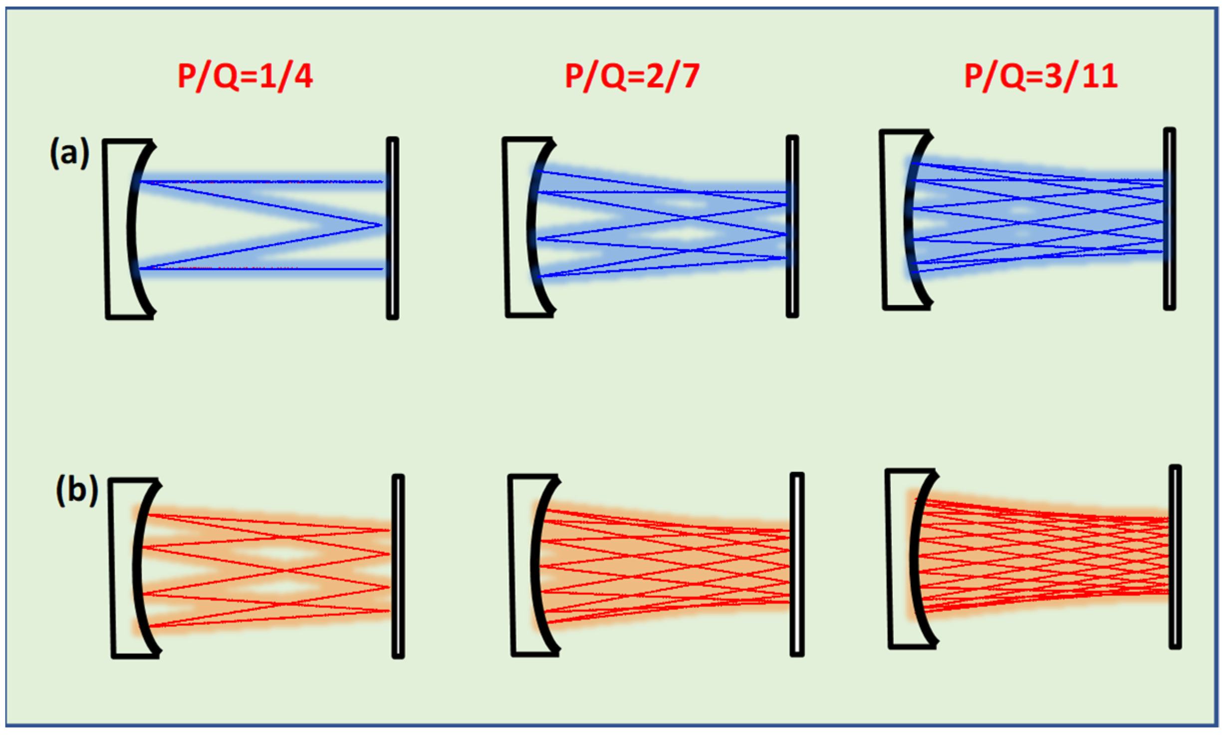
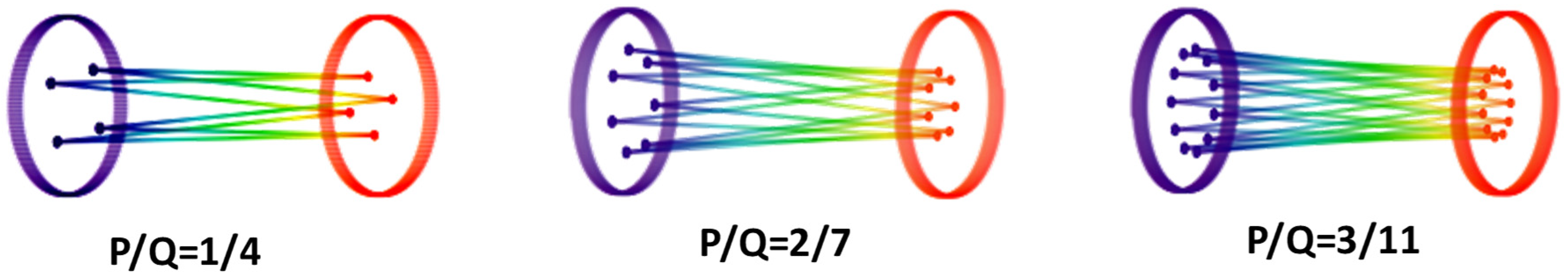
2.2. Parametric Equations for Geometric Rays

By using the propagation matrix for a degenerate cavity with $\Delta f_T/\Delta f_L=P/Q$, the characteristic equations for periodic ray trajectories can be verified as [18]

$$x_s(z)=W\left[\cos ({\theta }_s+{\varphi }_x)\mp \left(z/z_R\right)\sin ({\theta }_s+{\varphi }_x)\right]$$

(10)

where ${\theta }_s=(P/Q)2\pi s$, $s=0,1,2\cdots Q-1$ is the running index for the different rays, $z_R=(R_c/2)\sin \left[2\pi (\Delta f_T/\Delta f_L)\right]$ is the Rayleigh range, W is the amplitude of the transverse waist, ${\varphi }_x$ is associated with the initial condition, and − and + in the symbol of ∓ represent the leftward and rightward tracings, respectively. Let the amplitude $W=\sqrt{N_x}{w}_o$, Equation (10) can be expressed as

$$x_s(z)=\sqrt{N_x}\hspace{0.17em}w(z)\cos \left[{\theta }_s+{\varphi }_x\pm {\theta }_G\left(z\right)\right]$$

(11)

where $w(z)=w_0\sqrt{1+{(z/z_R)}^2}$ is the Gaussian beam parameter with the waist $w_o$, ${\theta }_G(z)={\tan }^{-1}(z/z_R)$ is the Gouy phase, and $N_x$ is the transverse order. Defining the dimensionless variable $\tilde{x}=\sqrt{2}x/w(z)$, the ray equation in Equation (11) can be given by ${\tilde{x}}_s(z)=\mathrm{Re}[\sqrt{2}\hspace{0.17em}{u}_s^{\pm }(z)]$ with

$$u_s^{\pm }(z)=\sqrt{N_x}\hspace{0.17em}\exp \left\{-i\hspace{0.17em}[{\theta }_s+{\varphi }_x\pm {\theta }_{\mathrm{G}}(z)]\right\}$$

(12)

In the spherical cavity, the properties for the x- and y-direction are the same. Therefore, the trajectory equation for the y-direction can be expressed as ${\tilde{y}}_s(z)=\mathrm{Re}[\sqrt{2}\hspace{0.17em}{v}_s^{\pm }(z)]$ with

$$v_s^{\pm }(z)=\sqrt{N_y}\hspace{0.17em}\exp \left\{-i\hspace{0.17em}[{\theta }_s+{\varphi }_y\pm {\theta }_{\mathrm{G}}(z)]\right\}$$

(13)

where $\tilde{y}=\sqrt{2}y/w(z)$, ${\varphi }_y$ is associated with the initial position, and $N_y$ is the transverse order. If one of the $N_x$ and $N_y$ is zero, the ray traces form a planar periodic orbit. For convenience, we set $N_x=0$ to discuss the feature of planar periodic orbits. Figure 2a shows the planar periodic orbits in the yz plane for $P/Q$ = 1/4, 2/7, and 3/11 with ${\varphi }_y=0$. The planar periodic orbits can be seen to be the reciprocating paths. It can be confirmed that if the phase factor ${\varphi }_y$ is the integer multiple of π/Q, the planar periodic tracing is a reciprocating type. On the other hand, when ${\varphi }_y$ is not the integer multiple of π/Q, the planar tracing is a generic type, as an example seen in Figure 2b for ${\varphi }_y=\pi /(2Q)$. The total numbers of rays for the reciprocating and generic periodic orbits can be easily found to be Q and 2Q, respectively. In addition to planar orbits, when both of $N_x$ and $N_y$ are not zero and ${\varphi }_x\ne {\varphi }_y$, the ray orbits are generally nonplanar, as shown in Figure 3 for $P/Q$ = 1/4, 2/7, and 3/11 with $N_x=N_y$ and ${\varphi }_x-{\varphi }_y=\pi /2$. The total number of rays in the nonplanar orbits can be seen to be Q.

2.3. Wave Representation for Unifying the Eigenmodes and Geometric Modes

In this section, we review that the Gaussian wave-packet state can be developed from the coherent state of quantum harmonic oscillator to unify the representation for the HG eigenmodes and geometric modes. From quantum theory, the coherent state for the one-dimensional (1D) harmonic oscillator is given by [58]

$$\begin{array}{ll}g(x;u)& ={\displaystyle \sum _{n=0}^{\infty }\frac{u^n}{\sqrt{n!}}{e}^{-|u{|}^2/2}\hspace{0.17em}{\psi }_n(x)}\\ & =\hspace{0.17em}{\pi }^{-1/4}\hspace{0.17em}{e}^{-(x^2-2\sqrt{2}xu+u^2+|u{|}^2)/2}\\ & =\hspace{0.17em}{\pi }^{-1/4}\hspace{0.17em}{e}^{i\hspace{0.17em}\mathrm{Im}(u)\hspace{0.17em}[\sqrt{2}x-\mathrm{Re}(u)]}\hspace{0.17em}{e}^{-{[x-\mathrm{Re}(\sqrt{2}u)]}^2/2}\end{array}$$

(14)

where ${\psi }_n(x)$ is the HG eigenstates given by

$${\psi }_n(x)={(2^{n}n!)}^{-1/2}{\pi }^{-1/4}{H}_n(x)\hspace{0.17em}{e}^{-x^2/2}$$

(15)

$H_n(·)$ are the Hermite polynomials of order n, and u is a complex parameter related to the moving path. The maximal point of the Gaussian coherent state $g(x;u)$ in Equation (14) is just at $x=\mathrm{Re}(\sqrt{2}u)$. The 2D HG eigenmodes in a spherical cavity with the transverse orders of n_x and n_y are given by [1]

$${\mathsf{\Phi }}_{n_x,n_y}^{\pm }(r)=\hspace{0.17em}{e}^{-i\hspace{0.17em}\hspace{0.17em}{\mathsf{\Theta }}^{\pm }(r)}\hspace{0.17em}{\psi }_{n_x}(\tilde{x})\hspace{0.17em}{e}^{\mp i\hspace{0.17em}{n}_x\hspace{0.17em}{\theta }_G(z)}\hspace{0.17em}{\psi }_{n_y}(\tilde{y})\hspace{0.17em}{e}^{\mp i\hspace{0.17em}{n}_y\hspace{0.17em}{\theta }_G(z)}$$

(16)

$${\mathsf{\Theta }}^{\pm }(r)=\hspace{0.17em}\frac{z}{z_R}\frac{{\tilde{x}}^2+{\tilde{y}}^2}{2}\pm {\theta }_G(z)$$

(17)

where ${\mathsf{\Theta }}^{\pm }(r)$ comprises the quadratic phase and Gouy phase, $r=(\tilde{x},\tilde{y},z)$, and the symbol of ± represents the propagating directions. From Equation (16), the transverse part of the HG mode can be given by $\hspace{0.17em}{\psi }_{n_x,n_y}^{(HG)}(\tilde{x},\tilde{y})={\psi }_{n_x}(\tilde{x})\hspace{0.17em}{\psi }_{n_y}(\tilde{y})$. Using Equations (12)–(17), the 2D Gaussian wave-packet state with the maximal point at ${\tilde{x}}_s(z)=\mathrm{Re}[\sqrt{2}\hspace{0.17em}{u}_s^{\pm }(z)]$ and ${\tilde{y}}_s(z)=\mathrm{Re}[\sqrt{2}\hspace{0.17em}{v}_s^{\pm }(z)]$ in Equations (12) and (13) can be generalized as

$$G(r;u_s^{\pm },v_s^{\pm })=\hspace{0.17em}{e}^{-i\hspace{0.17em}{\mathsf{\Theta }}^{\pm }(r)}g(\tilde{x};u_s^{\pm })\hspace{0.17em}g(\tilde{y};v_s^{\pm })$$

(18)

The Gaussian wave-packet state $G(r;u_s^{\pm },v_s^{\pm })$ can be seen to be the product of two 1D quantum coherent states except for the phase term $\exp [-i {\mathsf{\Theta }}^{\pm }(r)]$. In terms of $G(r;u_s^{\pm },v_s^{\pm })$, the wave representation for the geometric mode with the leftward and rightward parts of a complete tracing can be expressed as [18]

$${\mathsf{\Psi }}_{N_x,N_y}^{\pm }(r)=\frac{1}{Q}{\displaystyle \sum _{s=0}^{Q-1}\hspace{0.17em}G(r;u_s^{\pm },v_s^{\pm })\hspace{0.17em}{e}^{i(N_x\hspace{0.17em}+N_y)\hspace{0.17em}{\theta }_s\hspace{0.17em}}}$$

(19)

where the phase term $\exp [i(N_x\hspace{0.17em}+N_y)\hspace{0.17em}{\theta }_s]$ indicates the phase arising from the transverse component. From Equation (19), the intensity of the geometric mode within $-L_c\le z\le 0$ can be calculated by $I(r)={\left|{\mathsf{\Psi }}_{N_x,N_y}^{+}(r)\right|}^2+{\left|{\mathsf{\Psi }}_{N_x,N_y}^{-}(r)\right|}^2$, where the intensity emitted from the output coupler only considers the forward part ${\left|{\mathsf{\Psi }}_{N_x,N_y}^{+}(r)\right|}^2$.

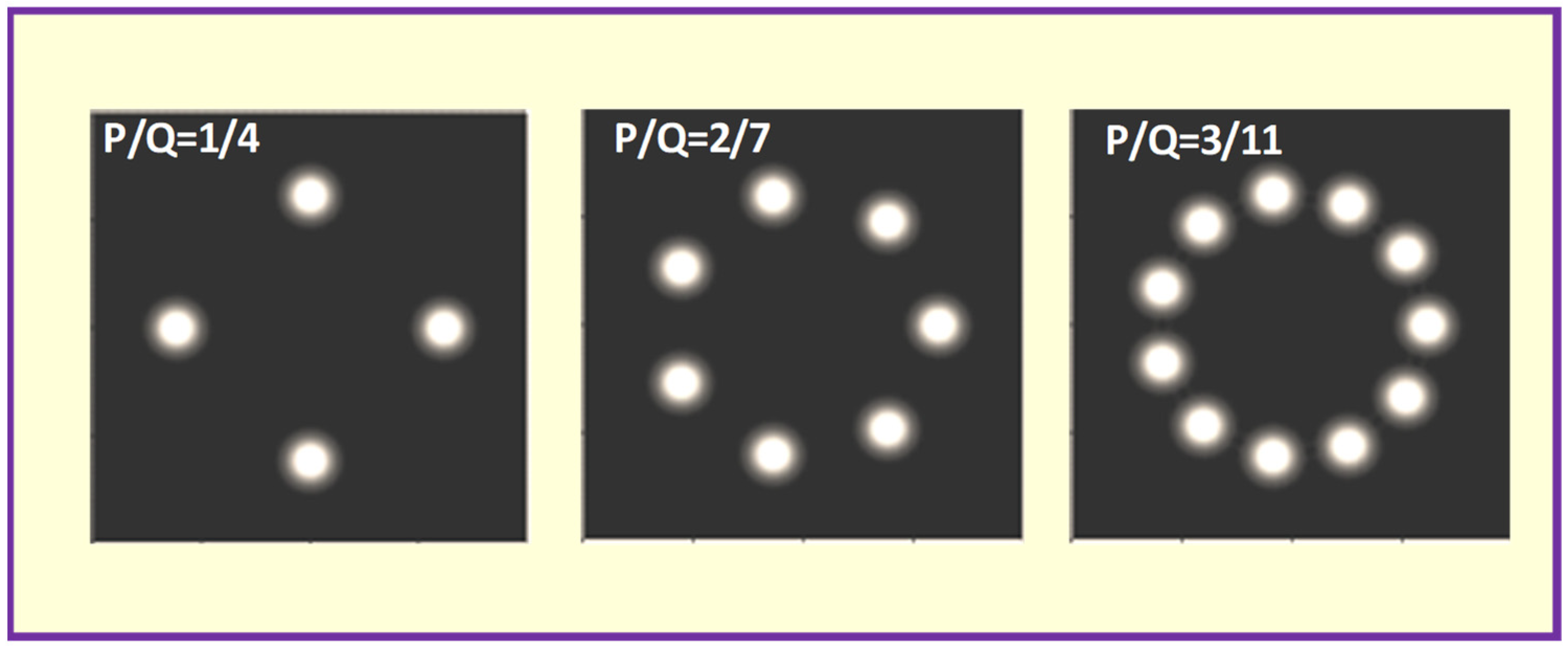
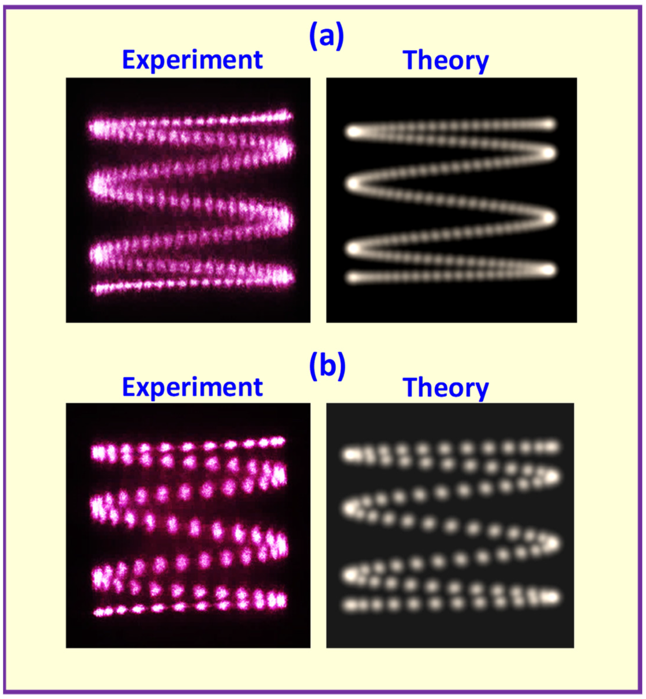
2.4. Experimental Results and Theoretical Confirmations

The experimental setup was a diode-end-pumped Nd:YVO₄ laser with a concave–flat cavity. The gain medium was an a-cut 2.0 at.% Nd:YVO₄ crystal with a length of 2 mm and an aperture of 10 × 10 mm². The aperture size of the used Nd:YVO₄ crystal was much larger than the conventional one for generating the transverse modes as high as possible. Both end surfaces of the Nd:YVO₄ crystal were coated as antireflective at 1064 nm (R < 0.2%). The laser crystal was wrapped with indium foil and mounted into a copper holder with water cooling. A concave mirror with a radius-of-curvature of 20 mm was employed as the input mirror whose entrance face was coated as antireflective at the pump wavelength of 808 nm and the second surface was coated as highly reflective at 1064 nm (R > 99.8%) and highly transmissive at 808 nm (T > 95%). A flat mirror with a partial reflection of 97% at 1064 nm was used as the output coupler. The pump source was a 3.0 W 808 nm fiber-coupled laser diode. The core diameter and the numerical aperture of the coupled fiber were 100 μm and 0.16, respectively. The laser crystal was placed behind the input mirror 1–2 mm. The pump beam from the fiber output was focused into the laser crystal with an average pump radius of approximately w_p = 100 μm.

The wave-packet state ${\mathsf{\Psi }}_{N_x,N_y}^{\pm }(r)$ in Equation (19) can reveal the spatial structure with ray-wave duality. Moreover, the state ${\mathsf{\Psi }}_{N_x,N_y}^{\pm }(r)$ can unify the representation for HG eigenmodes and geometric modes. Let us set $N_x=0$ and $N_y=N$ to demonstrate the geometric modes associated with the planar rays. From Equation (12), $N_x=0$ indicates $u_s^{\pm }=0$ and $g(x;0)={\psi }_0(x)$. As a result, Equation (19) becomes

$${\mathsf{\Psi }}_{0,N}^{\pm }(r)=\frac{1}{Q}{e}^{-i\hspace{0.17em}{\mathsf{\Theta }}^{\pm }(r)}{\psi }_0(\tilde{x})\hspace{0.17em}{\displaystyle \sum _{s=0}^{Q-1} g(\tilde{y},v_s^{\pm })\hspace{0.17em}{e}^{i\hspace{0.17em}N\hspace{0.17em}{\theta }_s}}$$

(20)

Figure 4 depicts the calculated patterns $I(r)={\left|{\mathsf{\Psi }}_{0,N}^{+}(r)\right|}^2+{\left|{\mathsf{\Psi }}_{0,N}^{-}(r)\right|}^2$ by using Equation (20) with $N=100$ to correspond to the trajectories shown in Figure 2. The calculated distributions agree very well with the geometric rays for all cases. On the other hand, if the transverse order N is not high enough, the distribution cannot exhibit the ray feature. When $N<Q/2$, the mathematical form of ${\mathsf{\Psi }}_{0,N}^{\pm }(r)$ can be verified to approach to the HG mode ${\psi }_{0,N}^{(HG)}(\tilde{x},\tilde{y})$, as discussed later.

By using Equation (20), the calculated far-field patterns $I(\tilde{x},\tilde{y})={\left|{\mathsf{\Psi }}_{0,N}^{+}(\tilde{x},\tilde{y},\tilde{z}=20)\right|}^2$ with $P/Q=2/7$, ${\varphi }_y=0$, and $\tilde{z}=z/z_R$ are shown in Figure 5a. The values of N in Figure 5a cover from 0 to 370 to display the variation from the HG modes to the geometric modes. The experimental results are shown in Figure 5b for comparison. The experimental results were obtained by using a diode-pumped solid-state laser with the off-axis pumping [4,14,15,16]. The experimental results agree very well with the calculated patterns for the variation from the HG modes to the geometric modes. Note that the transverse order N can be determined from ∆y by finding the integer closest to ${(\Delta y/{\omega }_c)}^2$, where ω_c is the fundamental mode size in the gain medium.

For a nondegenerate cavity, corresponding to $Q\to \infty$, we can confirm that the state ${\mathsf{\Psi }}_{0,N}^{\pm }(r)$ is directly related to the HG mode ${\psi }_{0,N}^{(HG)}(\tilde{x},\tilde{y})$. For $Q\to \infty$, the summation in Equation (20) can be rewritten as the integration:

$${\mathsf{\Psi }}_{0,N}^{\pm }(r)=\frac{1}{2\pi }{e}^{-i\hspace{0.17em}{\mathsf{\Theta }}^{\pm }(r)}{\psi }_0(\tilde{x})\hspace{0.17em}{\displaystyle {\int }_0^{2\pi }g(\tilde{y},v^{\pm })\hspace{0.17em}{e}^{i\hspace{0.17em}N\theta }d\theta }$$

(21)

with

$$v_{}^{\pm }(\theta )=\sqrt{N}\hspace{0.17em}\exp \left\{-i\hspace{0.17em}[\theta +{\varphi }_y\pm {\theta }_{\mathrm{G}}(z)]\right\}$$

(22)

Applying the orthogonal property

$$\frac{1}{2\pi }{\displaystyle {\int }_{\hspace{0.17em}0}^{2\pi }{e}^{i(n-m)\theta }d\theta }=\hspace{0.17em}{\delta }_{n,m}$$

(23)

to Equation (14), we can obtain

$$\frac{1}{2\pi }{\displaystyle {\int }_0^{\hspace{0.17em}2\pi }g(\tilde{y},v^{\pm })\hspace{0.17em}{e}^{iN\hspace{0.17em}\theta }\hspace{0.17em}d\theta }=\hspace{0.17em}{a}_N\hspace{0.17em}{e}^{-iN{\varphi }_y}\hspace{0.17em}{e}^{\mp i\hspace{0.17em}N\hspace{0.17em}{\theta }_G(\tilde{z})}\hspace{0.17em}{\psi }_N(\tilde{y})$$

(24)

Equation (24) implies that the Gaussian wave packet $g(\tilde{y},v^{\pm })$ can be used to express the eigenmodes ${\psi }_N(\tilde{y})$ with an integral transformation. Substituting Equation (24) into Equation (21), we can obtain

$$\underset{Q\to \infty }{\lim }{\mathsf{\Psi }}_{0,N}^{\pm }(r)=a_N\hspace{0.17em}{e}^{-i\hspace{0.17em}{\mathsf{\Theta }}^{\pm }(r)}\hspace{0.17em}\hspace{0.17em}{e}^{-iN{\varphi }_y}\hspace{0.17em}{e}^{\mp i\hspace{0.17em}N\hspace{0.17em}{\theta }_G(\tilde{z})}\hspace{0.17em}{\psi }_{0,N}^{(HG)}(\tilde{x},\tilde{y})$$

(25)

where $a_N=N^{N/2}{e}^{-N/2}/\sqrt{N!}$. Equation (25) means that the origin of HG eigenmodes is related to a nondegenerate cavity under the off-axis local pumping. Figure 6 shows the calculated patterns for $|{\mathsf{\Psi }}_{0,N}^{\pm }(r){|}^2$ and $|{\psi }_{0,N}^{(HG)}(\tilde{x},\tilde{y}){|}^2$ with different values of Q and P = 1 for N = 6 to manifest the asymptotic property in Equation (24).

Besides the planar rays, the representation in Equation (19) can be extended to the nonplanar tracings. The calculated results by using Equation (19) with $N_x=N_y=50$ for the transverse patterns on the flat mirror are shown in Figure 7, all the cases one-to-one corresponding to the nonplanar geometric modes shown in Figure 3. The calculated results are in good agreement with the geometric spots for all cases. Similar to the planar modes, if the transverse orders $N_x$ and $N_y$ are less than Q, the wave intensity cannot be localized on the geometric rays. For $N<Q/2$, the state ${\mathsf{\Psi }}_{N,N}^{\pm }(r)$ with ${\varphi }_x-{\varphi }_y=\pi /2$ can be found to exhibit the spatial pattern very close to the LG mode. Figure 8 shows the calculated transverse patterns of ${\mathsf{\Psi }}_{N,N}^{\pm }(r)$ on the flat mirror with $P/Q=2/7$ and ${\varphi }_x-{\varphi }_y=\pi /2$ for N = 1, 3, 14 to reveal the variation from the LG modes to the geometric modes. The present demonstration can be extended to the elliptical mode by considering ${\varphi }_x-{\varphi }_y\ne \pi /2$.

3. Spherical Cavity with Astigmatism

3.1. Eigenfrequency Spectrum and Lissajous Geometric Modes

Next, we review the eigenfrequency spectrum subject to the influence of a gain medium with birefringence. In the vicinity of $L_{P/Q}$, let the cavity length be given by $L_c=L_{P/Q}+\delta L_c$. The variation of the ratio $\Delta f_T/\Delta f_L$ due to an infinitesimal change $\delta L_c$ can be verified as

$$\delta \left(\frac{\Delta f_T}{\Delta f_L}\right)=\frac{\delta L_c}{\pi R_c\sin (2\pi P/Q)}$$

(26)

In terms of the Rayleigh range $z_R=(R_c/2)\sin (2\pi P/Q)$, the frequency ratio $\Delta f_T/\Delta f_L$ for the cavity length near $L_{P/Q}$ can be approximated as

$$\frac{\Delta f_T}{\Delta f_L}=\frac{P}{Q}+\frac{\delta L_c}{2\pi z_R}$$

(27)

Nd-doped vanadate crystals are frequently utilized as gain materials for implementing diode-pumped solid-state lasers. Due to the large birefringence, the Nd-doped vanadate crystal unavoidably leads to significant astigmatism inside the resonator without compensation. Consequently, there is a considerable difference between the effective cavity lengths $L_{c,x}$ and $L_{c,y}$, where $L_{c,x}$ and $L_{c,y}$ are the effective cavity lengths for the transverse parts in the directions of x//b and y//c, respectively. By using the new variables of $d=L_{c,y}-L_{c,x}$ and $L_c=(L_{c,y}+L_{c,x})/2$, the frequency ratios for x and y directions can be individually given by

$$\frac{\Delta f_{T,x}}{\Delta f_L}=\frac{1}{\pi }{\sin }^{-1}\left[\sqrt{\frac{1}{R_c}\left(L_c-\frac{d}{2}\right)}\right]$$

(28)

$$\frac{\Delta f_{T,y}}{\Delta f_L}=\frac{1}{\pi }{\sin }^{-1}\left[\sqrt{\frac{1}{R_c}\left(L_c+\frac{d}{2}\right)}\right]$$

(29)

The difference between $\Delta f_{T,x}$ and $\Delta f_{T,y}$ leads the relative eigenfrequency spectrum to be

$$F(\delta n;\hspace{0.17em}{L}_c,d)=\delta n_1\frac{\Delta f_{T,x}}{\Delta f_L}+\delta n_2\frac{\Delta f_{T,y}}{\Delta f_L}+\delta n_3$$

(30)

The calculated results for the relative spectrum $F(\delta n;\hspace{0.17em}{L}_c,d)$ as a function of $L_c/R_c$ for $\left|\delta n_i\right|\le 10$ with $i=1,2,3$ are shown in Figure 9. The values of $d/R_c$ used in Figure 9a,b are 3.3 × 10⁻³ and 6.6 × 10⁻³, respectively. It can be found that the astigmatism causes the degeneracies at $L_c=L_{P/Q}$ to split. Furthermore, the width of the frequency splitting can be seen to increase with increasing the value of d that measures the degree of astigmatism. Even though the astigmatism destroys the original degeneracies at $L_c=L_{P/Q}$, a variety of new fine degeneracies can be generated in the vicinity, as shown in Figure 9c for the cavity length near $P/Q=1/4$.

Equations (27)–(29) can be exploited to obtain the cavity lengths for the new fine degeneracies. From Equations (27)–(29), the frequency spacings $\Delta f_{T,x}$ and $\Delta f_{T,y}$ for the cavity length near $L_{P/Q}$ can be explicitly approximated as

$$\frac{\Delta f_{T,x}}{\Delta f_L}=\frac{P}{Q}+\frac{1}{2\pi z_R}\left(\delta L_c-\frac{d}{2}\right)$$

(31)

$$\frac{\Delta f_{T,y}}{\Delta f_L}=\frac{P}{Q}+\frac{1}{2\pi z_R}\left(\delta L_c+\frac{d}{2}\right)$$

(32)

Substituting Equations (31) and (32) into Equation (30), the cavity lengths for the new fine degeneracies can be derived from the condition of $F(\delta n;\hspace{0.17em}{L}_c,d)=0$. Accordingly, the requirements for the new degeneracies are

$$\frac{\delta n_1}{\delta n_2}=-\frac{\left(\delta L_c+d/2\right)}{\left(\delta L_c-d/2\right)}=\frac{p}{q}$$

(33)

$$(\delta n_1+\delta n_2)\left(P/Q\right)+\delta n_3=0$$

(34)

where p and q are integers. Equations (33) and (34) demand the integer pair $(p,q)$ to satisfy $p+q=QK$ with K to be an integer. Furthermore, the cavity length $\delta L_c$ with respect to $L_{P/Q}$ for the new degeneracy of $(p,q)$ can be obtained from Equation (33) as

$$\delta L_c=\frac{d}{2}\left(\frac{p-q}{p+q}\right)$$

(35)

Figure 10a–c shows the relative spectrum $F(\delta n;\hspace{0.17em}{L}_c,d)$ as a function of $\delta L_c/d$ for $\left|\delta n_i\right|\le 10$ with $i=1,2,3$ for three cases of $P/Q=$ 1/3, 2/5, and 3/8, respectively.

3.2. Parametric Equations for Lissajous Geometric Rays

From Equations (31), (32), and (35), the frequency spacings $\Delta f_{T,x}$ and $\Delta f_{T,y}$ for the new degeneracy $(p,q)$ can be rewritten as

$$\Delta f_{T,x}/\Delta f_L=\left(1-\beta q\right)(P/Q)$$

(36)

$$\Delta f_{T,y}/\Delta f_L=\left(1+\beta p\right)(P/Q)$$

(37)

where $\beta =d/(2\pi z_{R}KP)$. The transverse patterns of the high-order modes at the degeneracy $(p,q)$ have been observed to be localized on the Lissajous figures. Consequently, these observed modes are called the Lissajous geometric modes. The Rayleigh ranges for x and y directions can be given by

$$z_{R,x}=\frac{R_c}{2}\sin \left[2\pi (\Delta f_{T,x}/\Delta f_L)\right]$$

(38)

$$z_{R,y}=\frac{R_c}{2}\sin \left[2\pi (\Delta f_{T,y}/\Delta f_L)\right]$$

(39)

with $z_{R,x}$ and $z_{R,y}$, the beam waists are $w_{o,x}=\sqrt{\lambda z_{R,x}/\pi }$ and $w_{o,y}=\sqrt{\lambda z_{R,y}/\pi }$, where λ is the laser wavelength. In terms of $\Delta f_{T,x}$, $\Delta f_{T,y}$, $z_{R,x}$ and $z_{R,y}$, the parametric equations for an astigmatic cavity can be derived as [18,41]

$$x_s(z)=\sqrt{N_x}\hspace{0.17em}{w}_x(z)\cos \left[\left(2\pi s\right)\left(\Delta f_{T,x}/\Delta f_L\right)+{\varphi }_x\pm {\theta }_{G,x}\left(z\right)\right]$$

(40)

$$y_s(z)=\sqrt{N_y}\hspace{0.17em}{w}_y(z)\cos \left[\left(2\pi s\right)\left(\Delta f_{T,y}/\Delta f_L\right)+{\varphi }_y\pm {\theta }_{G,y}\left(z\right)\right]$$

(41)

where $\mathrm{s}=0, 1, 2, \cdots$ is the running index for different paths, $w_x\left(z\right)=w_{o,x}\sqrt{1+{(z/z_{R,x})}^2}$, $w_y\left(z\right)=w_{o,y}\sqrt{1+{(z/z_{R,y})}^2}$, ${\theta }_{G,x}\left(z\right){=\tan }^{-1}\left(z/z_{R,x}\right)$, and ${\theta }_{G,y}\left(z\right){=\tan }^{-1}\left(z/z_{R,y}\right)$, ${\varphi }_x$ and ${\varphi }_y$ are associated with the initial condition, $N_x$ and $N_y$ are the transverse orders in the x- and y-directions, and − and + in the symbol of ± correspond to the backward and forward rays, respectively.

The parameter β for the geometric mode needs to be a rational number $m/M$ for forming a complete orbit with finite rays, where m and M are coprime positive integers. By using $\beta =m/M$, the mode spacings $\Delta f_{T,x}$ and $\Delta f_{T,y}$ for the degeneracy $(p,q)$ are given by

$$\Delta f_{T,x}/\Delta f_L=(P{M}_x)/(QM)$$

(42)

$$\Delta f_{T,y}/\Delta f_L=(P{M}_y)/(QM)$$

(43)

where $M_x=M-mq$ and $M_y=M+mp$. Substituting Equations (42) and (43) into Equations (40) and (41), the parametric equations for the periodic rays of the Lissajous geometric mode related to the degeneracy $(p,q)$ in the vicinity of $L_{P/Q}$ could be derived as

$$x_s(z)=\sqrt{N_x}\hspace{0.17em}{w}_x(z)\cos \left[{\theta }_{q,s}+{\varphi }_x\pm {\theta }_{G,x}\left(z\right)\right]$$

(44)

$$y_s(z)=\sqrt{N_y}\hspace{0.17em}{w}_y(z)\cos \left[{\theta }_{p,s}+{\varphi }_y\pm {\theta }_{G,y}\left(z\right)\right]$$

(45)

where $s=0,1,2,\cdots ,MQ-1$ is the running index, ${\theta }_s=2\pi s(P/Q)$, ${\theta }_{q,s}={\theta }_s(M-mq)/M$, ${\theta }_{p,s}={\theta }_s(M+mp)/M$, $w_x(z)=w_{o,x}\sqrt{1+{(z/z_{R,x})}^2}$, $w_y(z)=w_{o,y}\sqrt{1+{(z/z_{R,y})}^2}$, ${\theta }_{G,x}(z)={\tan }^{-1}(z/z_{R,x})$, and ${\theta }_{G,y}(z)={\tan }^{-1}(z/z_{R,y})$. The total ray number for forming a geometric period is $MQ$. Typically, the value of M ranges from 10² to 10⁴.

3.3. Wave Representation for Lissajous Geometric Modes

Next, we review that the parametric equations in Equations (44) and (45) for geometric rays can be implanted into the coherent state in Equation (14) to derive the Gaussian wave-packet representation for Lissajous geometric modes. By using the dimensionless variables $\tilde{x}=\sqrt{2}x/w_x(z)$ and $\tilde{y}=\sqrt{2}y/w_y(z)$, the parametric equations in Equations (44) and (45) can be written as ${\tilde{x}}_s(z)=\mathrm{Re}[\sqrt{2}\hspace{0.17em}{u}_s^{\pm }(z)]$ and ${\tilde{y}}_s(z)=\mathrm{Re}[\sqrt{2}\hspace{0.17em}{v}_s^{\pm }(z)]$ with

$$u_s^{\pm }(z)=\sqrt{N_x}\hspace{0.17em}\exp \left\{-i\hspace{0.17em}\left[{\theta }_{q,s}+{\varphi }_x\pm {\theta }_{G,x}\left(z\right)\right]\right\}$$

(46)

$$v_s^{\pm }(z)=\sqrt{N_y}\hspace{0.17em}\exp \left\{-i\hspace{0.17em}\left[{\theta }_{p,s}+{\varphi }_y\pm {\theta }_{G,y}\left(z\right)\right]\right\}$$

(47)

Considering the effect of astigmatism in Equations (16)–(19), these equations for the HG eigenmode and geometric modes are revised as

$${\mathsf{\Phi }}_{n_x,n_y}^{\pm }(r)=\hspace{0.17em}{e}^{-i\hspace{0.17em}\hspace{0.17em}{\mathsf{\Theta }}^{\pm }(r)}\hspace{0.17em}{\psi }_{n_x}(\tilde{x})\hspace{0.17em}{e}^{\mp i\hspace{0.17em}{n}_x\hspace{0.17em}{\theta }_{G,x}(z)}\hspace{0.17em}{\psi }_{n_y}(\tilde{y})\hspace{0.17em}{e}^{\mp i\hspace{0.17em}{n}_y\hspace{0.17em}{\theta }_{G,y}(z)}$$

(48)

$${\mathsf{\Theta }}^{\pm }(r)=\hspace{0.17em}\frac{1}{2}\left\{\left[{\tilde{x}}^2\left(\frac{z}{z_{R,x}}\right)+{\tilde{y}}^2\left(\frac{z}{z_{R,y}}\right)\right]\pm \left[{\theta }_{G,x}(z)+{\theta }_{G,y}(z)\right]\right\}$$

(49)

$$G(r;u_s^{\pm },v_s^{\pm })=\hspace{0.17em}{e}^{-i\hspace{0.17em}{\mathsf{\Theta }}^{\pm }(r)}g(\tilde{x};u_s^{\pm })\hspace{0.17em}g(\tilde{y};v_s^{\pm })$$

(50)

$${\mathsf{\Psi }}_{N_x,N_y}^{\pm }(r)=\frac{1}{MQ}{\displaystyle \sum _{s=0}^{MQ-1}\hspace{0.17em}G(r;u_s^{\pm },v_s^{\pm })\hspace{0.17em}{e}^{i(N_x\hspace{0.17em}{\theta }_{q,s}+N_y\hspace{0.17em}{\theta }_{p,s})\hspace{0.17em}}}$$

(51)

Equations (49)–(51) stand for the Gaussian wave-packet representation for the Lissajous geometric modes.

The spatial characteristics of Lissajous geometric modes can be deeply comprehended from the parametric equations in Equations (44) and (45) and the wave representation in Equations (49)–(51). We can use Equations (44) and (45) to verify that the total number of output rays is $N=MQ/C_d$, where $C_d$ is the common divisor among $\left(M-qm\right)$, $\left(M+pm\right)$, and MQ. The total path length on the transverse plane for Lissajous geometric modes can be expressed as

$$L_{p,q}(N_x,N_y;z)={\displaystyle {\int }_0^{2\pi }\sqrt{\hspace{0.17em}{\left[\frac{dx(\theta ;z)}{d\theta }\right]}^2+{\left[\frac{dy(\theta ;z)}{d\theta }\right]}^2}d\theta }$$

(52)

where

$$x(\theta ;z)=\sqrt{N_x}\hspace{0.17em}{w}_x(z)\cos \left[q(\theta +{\varphi }_x)\right]$$

(53)

$$y(\theta ;z)=\sqrt{N_y}\hspace{0.17em}{w}_y(z)\cos [p(\theta +{\varphi }_y)]$$

(54)

Numerical calculations revealed that the path length $L_{p,q}(N_x,N_y;z)$ relies primarily on the parameters $\left(p,q\right)$ and $\left(N_x,N_y\right)$ and is nearly independent of the phase factors $({\varphi }_x,{\varphi }_y)$. Moreover, the path length $L_{p,q}(N_x,N_y;z)$ can be accurately approximated with

$$L_{p,q}(N_x,N_y;z)=4\sqrt{q^2{N}_x{w}_x^2(z)+p^2{N}_y{w}_y^2(z)}$$

(55)

Since both values of $w_x\left(z\right)$ and $w_y\left(z\right)$ are rather close, we can use $\sqrt{2}{w}_x\left(z\right)\approx \sqrt{2}{w}_y\left(z\right)$ as the effective width of the Gaussian wave packets. Based on the number of Gaussian wave packets $N=MQ/C_d$ and the overall length $L_{p,q}(N_x,N_y;z)$ in Equation (55), the degree of the average overlapping between two contiguous Gaussian spots can be estimated as

$$D=\frac{\sqrt{2\hspace{0.17em}}\hspace{0.17em}n\hspace{0.17em}MQ/C_d}{4\sqrt{q^2{N}_x+p^2{N}_y}}$$

(56)

where n is the greatest common divisor of p and q. The value of n means the number of Lissajous curves appearing in the transverse plane of the corresponding geometric mode. When $D\gg 1$, the Gaussian wave packets in Equation (51) substantially overlap with each other to display a feature of continuous curves, not the original discrete spots. In contrast, when the value of D is considerably less than 1.0, the transverse pattern can be seen to reveal a feature of separate spots corresponding to geometric rays.

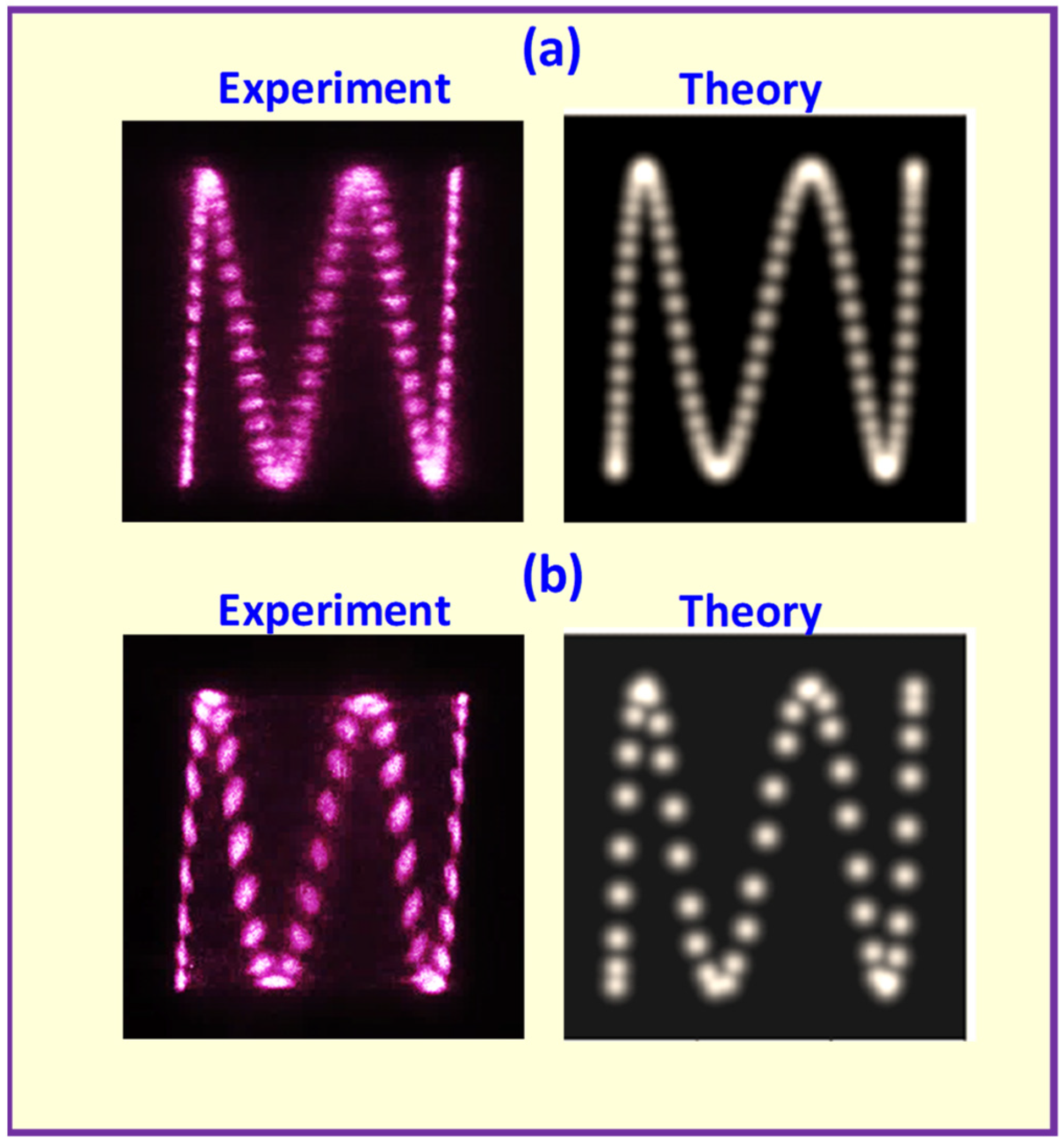
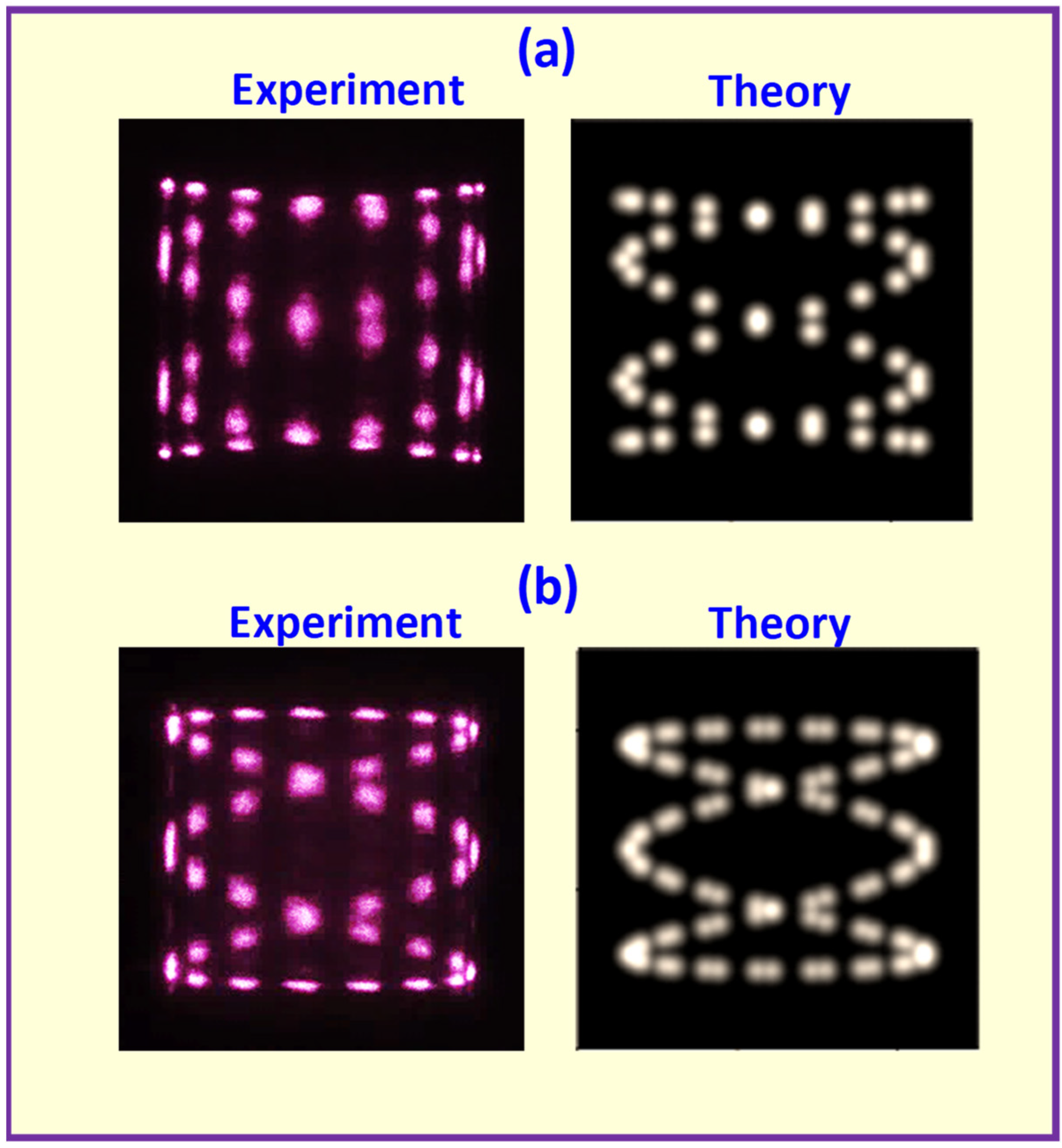
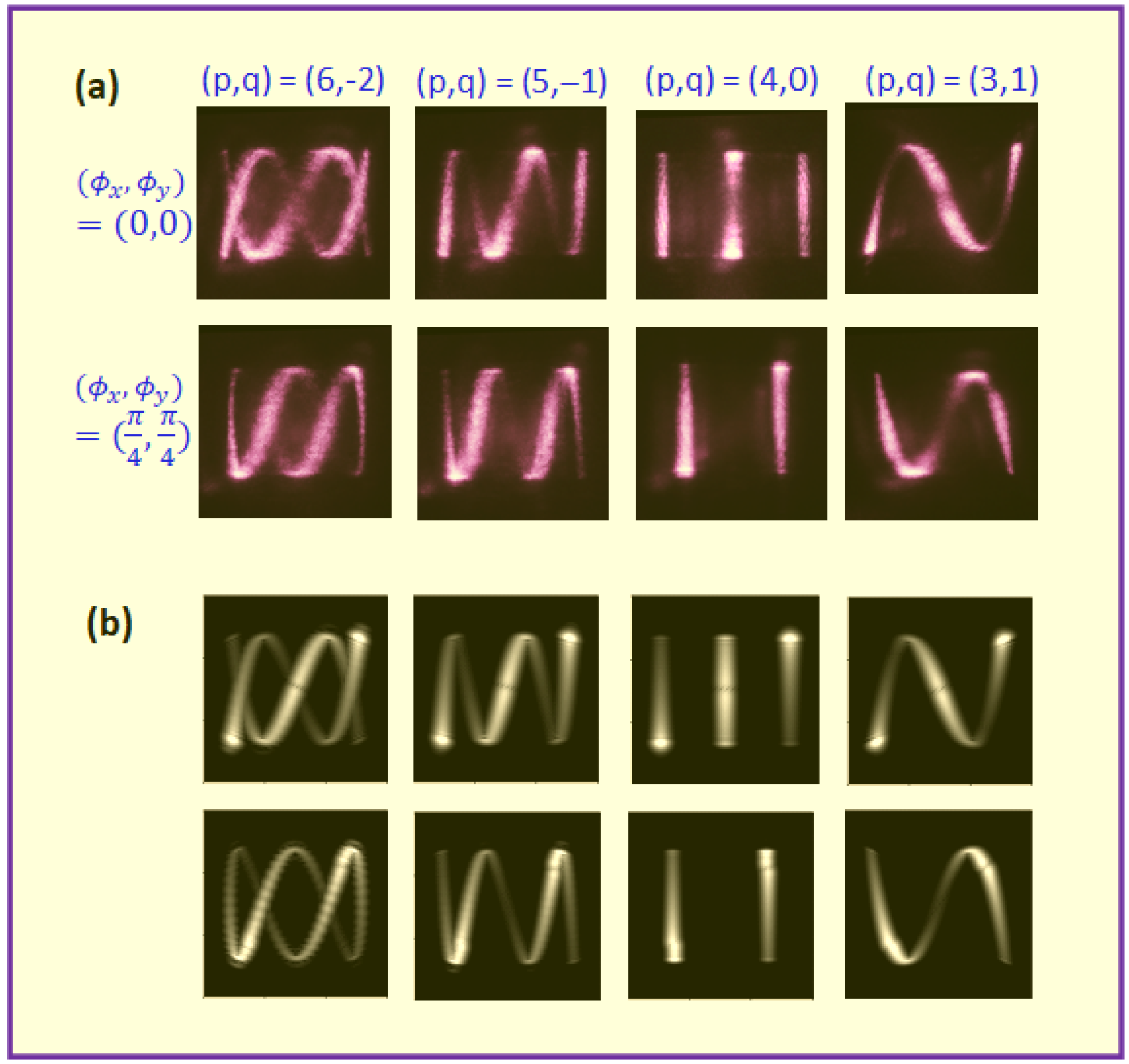
3.4. Experimental and Numerical Results

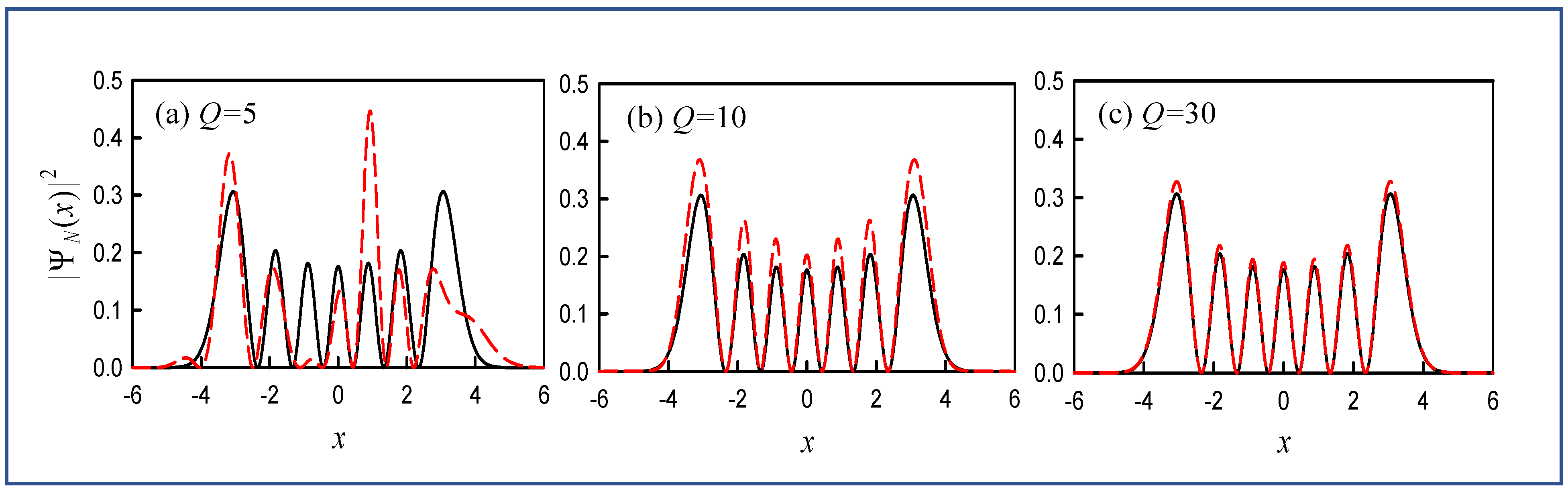
We present an overview of the comparison between experimental and theoretical results for Lissajous geometric modes. It has been demonstrated that Lissajous geometric modes can be well generated from an off-axis diode-end-pumped Nd:YVO₄ laser. The detailed description for the experiment can be obtained from previous papers [14,40,41]. When a short laser crystal with length of 1~2 mm was used in experiment, the value of M was found to be greater than 300 by far. Since the transverse orders of $N_x$ and $N_y$ for Lissajous lasing modes can be approximately ${10}^2~{10}^3$ by varying the off-axis displacement of the pumping, the degree of the overlapping D in Equation (56) is then significantly larger than 1.0. The first experimental case is shown in Figure 11a for the Lissajous geometric mode corresponding to the parameters of $\left(P,Q\right)=\left(1, 3\right)$, $\left(p,q\right)=\left(4,-1\right)$, and ${\varphi }_x={\varphi }_y=\pi /3$ for the transverse patterns with propagation dependence. The theoretical results are depicted in Figure 11b by using Equations (14), (46), (47), (50) and (51) with the parameters and $M=400$, $\left(N_x,N_y\right)=\left(400, 200\right)$, and $m=1$. Theoretical patterns can be seen to agree very well with experimental results. From Equation (56), the value of D for the case in Figure 11 can be obtained to be approximately 7.07. As expected, the transverse pattern displays a characteristic of continuous curve due to large overlapping between Gaussian wave packets.

The condition for the critical overlapping between Gaussian wave packets can be specified as $D=1$. Figure 12 shows the influence of the degree of the overlapping D on the transverse far-field patterns with the parameters of $\left(P,Q\right)=\left(1, 4\right)$, $\left(p,q\right)=\left(1, 7\right)$, ${\varphi }_x={\varphi }_y=0,$ $M=100$, and $m=1$. The values of $\left(N_x,N_y\right)$ in Figure 12a–d are $\left(200, 200\right)$, $\left(400, 400\right)$, $\left(600, 600\right)$, and $\left(800, 800\right)$, respectively. Accordingly, the values of D for Figure 12a–d are 1.414, 1.000, 0816, and 0.707, respectively. Figure 12 clearly reveals that the transverse pattern varies from the continuous curves to the discrete spots for the value of D from greater to less than 1.0.

Experimentally, the astigmatism needs to be increased to reduce the value of M for realizing the condition of $D<1$. One practical way of increasing the astigmatism is to use a gain medium with longer length. By using a length of 10 mm, the value of M can be reduced to the range between 40 and 120. In addition to reducing the value of M, Equation (56) indicates that the degree of the overlapping D can be varied by the factor $C_d$ which is the common divisor among $\left(M-qm\right)$, $\left(M+pm\right)$, and MQ. The influence of the factor $C_d$ is shown in Figure 13 for two cases of $M=100$ and $M=101$ for the far-field transverse patterns with the parameters of $\left(P,Q\right)=\left(1, 4\right)$, $\left(p,q\right)=\left(1, 7\right)$, $\left(N_x,N_y\right)=\left(500, 300\right)$, ${\varphi }_x={\varphi }_y=0,$ and $m=1$. All far-field patterns were measured at the position of $z=100 L_c$. The results in Figure 13a with $M=100$ can be found to correspond to $C_d=1$ and $D=0.898$. On the other hand, the case shown in Figure 13b with $M=101$ corresponds to $C_d=2$ and $D=0.454$. It can be found that even though the difference of the astigmatism is very small for $M=100$ and $M=101$, the degree of the overlapping D varies significantly due to the influence of the factor $C_d$. Figure 14a,b shows another similar example with $M=46$ and $M=47$, respectively. The cavity parameters are $\left(P,Q\right)=\left(1, 4\right)$, $\left(p,q\right)=\left(5,-1\right)$, $\left(N_x,N_y\right)=\left(300, 300\right)$, ${\varphi }_x={\varphi }_y=0,$ and $m=1$. Consequently, the values of D are 0.737 and 0.376 for Figure 14a,b, respectively. Experimental results can be seen to agree very well with theoretical results.

The results shown in Figure 13 and Figure 14 are for the cases with $n=1$. The value of n arising from the greatest common divisor of p and q determine the number of transverse Lissajous curves in the geometric mode. An example for the far-field transverse pattern with $n=2$ is depicted in Figure 15a with the parameters of $\left(P,Q\right)=\left(1, 4\right)$, $\left(p,q\right)=\left(-2, 6\right)$, $\left(N_x,N_y\right)=\left(300, 200\right)$, ${\varphi }_x={\varphi }_y=\pi /2$, $M=102$, and $m=1$. The result in Figure 15a corresponds to $C_d=4$ and $D=0.67$. Although the value of n determines the number of Lissajous curves in the geometric mode, some phase values of $\left({\varphi }_x,{\varphi }_y\right)$ may lead the corresponding curves to coincide together, as depicted in Figure 15b. All parameters for Figure 15a,b are the same except for ${\varphi }_x={\varphi }_y=\pi /4$. Once again, all theoretical results are in good agreement with experimental patterns.

4. Damping Effect

Experimental patterns shown in Figure 11, Figure 12, Figure 13, Figure 14 and Figure 15 were generated by using an output coupler with a transmission as low as 2% at the lasing wavelength. It has been experimentally observed that the spatial structures of lasing modes can be significantly affected by the transmission of the output coupler. It has been demonstrated [53] that an output coupler with high transmission can be used to deliberately generate the asymmetric lasing modes. In theory, the influence of output transmission on the spatial structures of Lissajous lasing modes can be directly taken into account from Equation (51). Let the effective damping coefficient be considered as a loss factor from the output transmission T_oc. The loss factor on the sth ray in Equation (51) can be given by $\exp (-\gamma {\theta }_s)$ with $\gamma =T_{oc}/2\pi$. Taking the damping effect into account, the Gaussian wave-packet representation for Lissajous geometric modes can be expressed as [38,53]

$${\mathsf{\Psi }}_{N_x,N_y}^{\pm }(r)=\frac{1}{MQ}{\displaystyle \sum _{s=0}^{MQ-1}\hspace{0.17em}G(r;u_s^{\pm },v_s^{\pm })\hspace{0.17em}{e}^{i(N_x\hspace{0.17em}{\theta }_{q,s}+N_y\hspace{0.17em}{\theta }_{p,s})\hspace{0.17em}}{e}^{-\gamma \hspace{0.17em}{\theta }_s}}$$

(57)

Figure 16a and Figure 17a show experimental results obtained, respectively, with $T_{oc}=2\%$ and 15% for the far-field patterns of Lissajous geometric modes with the cavity length near $\left(P,Q\right)=\left(1, 4\right)$ for four different (p, q). The first and second row in Figure 16a and Figure 17a are the cases for ${\varphi }_x={\varphi }_y=0$ and ${\varphi }_x={\varphi }_y=\pi /4$, respectively. Note that the far-field patterns were measured at the position of $z=50 L_c$. Making a comparison between the patterns of Figure 16a and Figure 17a, a high output transmission can lead the Lissajous transverse pattern to exhibit a feature of broken line. The asymmetric structure arising from a high output transmission can be found to depend on not only (p, q) but also $\left({\varphi }_x,{\varphi }_y\right)$. By using Equations (51) and (57), the calculated patterns corresponding to Figure 16a and Figure 17a are shown in Figure 16b and Figure 17b with experimental parameters and $M=200$, $\left(N_x,N_y\right)=\left(150, 100\right)$, and $m=1$. All the calculated patterns are in excellent agreement with experimental results to manifest the damping effect on the spatial structures of Lissajous geometric modes. Finally, experimental results for the far-field patterns of Lissajous geometric modes generated by using an output coupler with a higher transmission of $T_{oc}=25\%$ are shown in Figure 18a. By using Equation (57) with the parameters of $M=200$, $\left(N_x,N_y\right)=\left(75, 50\right)$, and $m=1$, theoretical patterns for $T_{oc}=25\%$ are calculated and shown in Figure 18b. The superiority of the Gaussian wave-packet representation can be confirmed from the good agreement between experimental and theoretical patterns in manifesting the damping effect arising from cavity losses.

5. Conclusions

We presented a thorough overview of the laser transverse modes with ray-wave duality in spherical cavities with and without astigmatism. We first reviewed the eigenfrequency spectrum in an ideal spherical cavity to manifest the critical role of degeneracy in the ray-wave correspondence. The derivation of Gaussian wave-packet states was given to understand the unification of the HG eigenmodes and the planar geometric modes. We extended the wave representation of the planar geometric modes to the case for the elliptical modes with orbital angular momentum. Furthermore, we reviewed the fine structure of the characteristic frequency in a spherical cavity with astigmatism. Taking the astigmatism into account, the wave packet representation for Lissajous geometric modes has been completely introduced. Finally, we reviewed the damping effect on the formation of transverse modes to reveal the generation of asymmetric geometric modes. It is believed that this review can offer useful insights into the ray-wave duality in mesoscopic optics and laser physics.

References

1. Haus, H.A. Waves and Fields in Optoelectronics; Prentice-Hall: Englewood Cliffs, NJ, USA, 1984. [Google Scholar]
2. Chen, Y.F.; Lee, C.C.; Wang, C.H.; Hsieh, M.X. Laser transverse modes of spherical resonators: A review [Invited]. Chin. Opt. Lett. 2020, 18, 091404. [Google Scholar] [CrossRef]
3. Boyd, G.D.; Kogelnik, H. Generalized Confocal Resonator Theory. Bell Syst. Tech. J. 1962, 41, 1347–1369. [Google Scholar] [CrossRef]
4. Chen, Y.F.; Huang, T.M.; Kao, C.F.; Wang, C.L.; Wang, S.C. Generation of Hermite-Gaussian modes in fiber-coupled la–ser-diode end-pumped lasers. IEEE J. Quantum Electron. 1997, 33, 1025–1031. [Google Scholar] [CrossRef]
5. Laabs, H.; Ozygus, B. Excitation of Hermite Gaussian modes in end-pumped solid-state lasers via off-axis pumping. Opt. Laser Technol. 1996, 28, 213–214. [Google Scholar] [CrossRef]
6. Chen, Y.F.; Chang, C.C.; Lee, C.Y.; Tung, J.C.; Liang, H.C.; Huang, K.F. Characterizing the propagation evolution of wave patterns and vortex structures in astigmatic transformations of Hermite–Gaussian beams. Laser Phys. 2017, 28, 015002. [Google Scholar] [CrossRef]
7. Chen, Y.F.; Lan, Y.P. Dynamics of the Laguerre Gaussian TEM*0,l mode in a solid-state laser. Phys. Rev. A 2001, 63, 063807. [Google Scholar] [CrossRef]
8. Flood, C.J.; Giuliani, G.; Van Driel, H.M. Preferential operation of an end-pumped Nd:YAG laser in high-order Laguerre–Gauss modes. Opt. Lett. 1990, 15, 215–217. [Google Scholar] [CrossRef] [PubMed]
9. Bisson, J.-F.; Senatsky, Y.; Ueda, K.-I. Generation of Laguerre-Gaussian modes in Nd:YAG laser using diffractive optical pumping. Laser Phys. Lett. 2005, 2, 327–333. [Google Scholar] [CrossRef]
10. Kim, J.; Clarkson, W.A. Selective generation of Laguerre–Gaussian (LG0n) mode output in a diode-laser pumped Nd:YAG laser. Opt. Commun. 2013, 296, 109–112. [Google Scholar] [CrossRef]
11. Lee, A.J.; Omatsu, T.; Pask, H.M. Direct generation of a first-Stokes vortex laser beam from a self-Raman laser. Opt. Express 2013, 21, 12401–12409. [Google Scholar] [CrossRef]
12. Dingjan, J.; van Exter, M.; Woerdman, J. Geometric modes in a single-frequency Nd:YVO4 laser. Opt. Commun. 2001, 188, 345–351. [Google Scholar] [CrossRef]
13. Chen, Y.F.; Jiang, C.H.; Lan, Y.P.; Huang, K.F. Wave representation of geometrical laser beam trajectories in a hemiconfocal cavity. Phys. Rev. A 2004, 69, 053807. [Google Scholar] [CrossRef]
14. Chen, Y.F.; Tung, J.C.; Chiang, P.Y.; Liang, H.C.; Huang, K.F. Exploring the effect of fractional degeneracy and the emer–gence of ray-wave duality in solid-state lasers with off-axis pumping. Phys. Rev. A 2013, 88, 013827. [Google Scholar] [CrossRef] [Green Version]
15. Tung, J.C.; Liang, H.C.; Tuan, P.H.; Chang, F.L.; Huang, K.F.; Lu, T.H.; Chen, Y.F. Selective pumping and spatial hole burning for generation of photon wave packets with ray-wave duality in solid-state lasers. Laser Phys. Lett. 2016, 13. [Google Scholar] [CrossRef]
16. Chen, Y.F.; Chang, C.C.; Lee, C.Y.; Sung, C.L.; Tung, J.C.; Su, K.W.; Liang, H.C.; Chen, W.D.; Zhang, G. High-peak-power large-angular-momentum beams generated from passively Q-switched geometric modes with astigmatic transformation. Photonics Res. 2017, 5, 561–566. [Google Scholar] [CrossRef]
17. Barré, N.; Romanelli, M.; Lebental, M.; Brunel, M. Waves and rays in plano-concave laser cavities: I. Geometric modes in the paraxial approximation. Eur. J. Phys. 2017, 38, 034010. [Google Scholar] [CrossRef]
18. Chen, Y.F.; Li, S.C.; Hsieh, Y.H.; Tung, J.C.; Liang, H.C.; Huang, K.F. Laser wave-packet representation to unify eigenmodes and geometric modes in spherical cavities. Opt. Lett. 2019, 44, 2649–2652. [Google Scholar] [CrossRef]
19. Tung, J.C.; Hsieh, Y.H.; Omatsu, T.; Huang, K.F.; Chen, Y.F. Generating laser transverse modes analogous to quantum Green’s functions of two-dimensional harmonic oscillators. Photon–Res. 2017, 5, 733. [Google Scholar] [CrossRef]
20. Chen, Y.F.; Tung, J.C.; Tuan, P.H.; Yu, Y.T.; Liang, H.C.; Huang, K.F. Characterizing classical periodic orbits from quantum Green’s functions in two-dimensional integrable systems: Harmonic oscillators and quantum billiards. Phys. Rev. E 2017, 95, 012217. [Google Scholar] [CrossRef] [Green Version]
21. Chen, Y.-F.; Tseng, Y.C.; Ke, H.T.; Hsieh, M.X.; Tung, J.-C.; Hsieh, Y.H.; Liang, H.-C.; Huang, K.F. High-power structured laser modes: Manifestation of quantum Green’s function. Opt. Lett. 2020, 45, 4579. [Google Scholar] [CrossRef]
22. Keski-Rahkonen, J.; Ruhanen, A.; Heller, E.J.; Räsänen, E. Quantum Lissajous Scars. Phys. Rev. Lett. 2019, 123, 214101. [Google Scholar] [CrossRef] [PubMed] [Green Version]
23. Huang, K.F.; Chen, Y.F.; Lai, H.C.; Lan, Y.P. Observation of the Wave Function of a Quantum Billiard from the Transverse Patterns of Vertical Cavity Surface Emitting Lasers. Phys. Rev. Lett. 2002, 89, 224102. [Google Scholar] [CrossRef] [PubMed]
24. Chen, C.C.; Liu, C.C.; Su, K.W.; Lu, T.H.; Chen, Y.F.; Huang, K.F. Statistical properties of experimental coherent waves in microcavity lasers: Analogous study of quantum billiard wave functions. Phys. Rev. E 2007, 75, 046202. [Google Scholar] [CrossRef] [Green Version]
25. Chen, C.C.; Yu, Y.T.; Chen, R.C.C.; Huang, Y.J.; Su, K.W.; Chen, Y.F.; Huang, K.F. Transient Dynamics of Coherent Waves Released from Quantum Billiards and Analogous Observation from Free-Space Propagation of Laser Modes. Phys. Rev. Lett. 2009, 102, 044101. [Google Scholar] [CrossRef] [Green Version]
26. Chen, Y.F.; Yu, Y.T.; Chiang, P.Y.; Tuan, P.H.; Huang, Y.J.; Liang, H.C.; Huang, K.F. Manifestation of quantum-billiard eigenvalue statistics from subthreshold emission of vertical-cavity surface-emitting lasers. Phys. Rev. E 2011, 83, 016208. [Google Scholar] [CrossRef] [Green Version]
27. Yu, Y.T.; Tuan, P.H.; Chang, K.C.; Hsieh, Y.H.; Huang, K.F.; Chen, Y.F. Exploiting broad-area surface emitting lasers to manifest the path-length distributions of finite-potential quantum billiards. Opt. Express 2016, 24, 82–91. [Google Scholar] [CrossRef] [PubMed]
28. Raghu, S.; Haldane, F.D.M. Analogs of quantum-Hall-effect edge states in photonic crystals. Phys. Rev. A 2008, 78, 033834. [Google Scholar] [CrossRef] [Green Version]
29. Chen, W.-J.; Jiang, S.-J.; Chen, X.-D.; Zhu, B.; Zhou, L.; Dong, J.-W.; Chan, C.T. Experimental realization of photonic topological insulator in a uniaxial metacrystal waveguide. Nat. Commun. 2014, 5, 5782. [Google Scholar] [CrossRef]
30. Brack, M.; Bhaduri, R.K. Semiclassical Physics; Addison-Wesley: Reading, MA, USA, 1997. [Google Scholar]
31. Courtois, J.; Mohamed, A.; Romanini, D. Degenerate astigmatic cavities. Phys. Rev. A 2013, 88. [Google Scholar] [CrossRef]
32. Habraken, S.J.M.; Nienhuis, G. Modes of a twisted optical cavity. Phys. Rev. A 2007, 75, 033819. [Google Scholar] [CrossRef] [Green Version]
33. Tung, J.C.; Tuan, P.H.; Liang, H.C.; Huang, K.F.; Chen, Y.F. Fractal frequency spectrum in laser resonators and three-dimensional geometric topology of optical coherent waves. Phys. Rev. A 2016, 94, 023811. [Google Scholar] [CrossRef] [Green Version]
34. Liang, H.-C.; Lin, H.-Y. Generation of resonant geometric modes from off-axis pumped degenerate cavity Nd:YVO4 lasers with external mode converters. Opt. Lett. 2020, 45, 2307–2310. [Google Scholar] [CrossRef]
35. Zhang, Q.; Ozygus, B.; Weber, H. Degeneration effects in laser cavities. Eur. Phys. J. Appl. Phys. 1999, 6, 293–298. [Google Scholar] [CrossRef]
36. Cao, H.; Wiersig, J. Dielectric microcavities: Model systems for wave chaos and non-Hermitian physics. Rev. Mod. Phys. 2015, 87, 61–111. [Google Scholar] [CrossRef]
37. Tung, J.C.; Liang, H.C.; Lu, T.H.; Huang, K.F.; Chen, Y.F. Exploring vortex structures in orbital-angular-momentum beams generated from planar geometric modes with a mode converter. Opt. Express 2016, 24, 22796. [Google Scholar] [CrossRef] [PubMed]
38. Chen, Y.F.; Lai, Y.-H.; Hsieh, M.X.; Hsieh, Y.H.; Tu, C.W.; Liang, H.C.; Huang, K.F. Wave representation for asymmetric elliptic vortex beams generated from the astigmatic mode converter. Opt. Lett. 2019, 44, 2028–2031. [Google Scholar] [CrossRef] [PubMed]
39. Chen, Y.F.; Lu, T.H.; Su, K.W.; Huang, K.F. Devil’s Staircase in Three-Dimensional Coherent Waves Localized on Lissajous Parametric Surfaces. Phys. Rev. Lett. 2006, 96, 213902. [Google Scholar] [CrossRef] [PubMed]
40. Tung, J.C.; Liang, H.C.; Lin, Y.C.; Su, K.W.; Huang, K.F.; Chen, Y.F. Power scale-up and propagation evolution of structured laser beams concentrated on 3D Lissajous parametric surfaces. Laser Phys. Lett. 2014, 11, 125806. [Google Scholar] [CrossRef]
41. Hsieh, M.X.; Zheng, X.L.; Yu, Y.T.; Liang, H.-C.; Huang, K.F.; Chen, Y.-F. Characterizing the spatial entanglement from laser modes analogous to quantum wave functions. Opt. Lett. 2021, 46, 3713–3716. [Google Scholar] [CrossRef]
42. Herriott, D.; Kogelnik, H.; Kompfner, R. Off-Axis Paths in Spherical Mirror Interferometers. Appl. Opt. 1964, 3, 523–526. [Google Scholar] [CrossRef] [Green Version]
43. Herriott, D.R.; Schulte, H.J. Folded Optical Delay Lines. Appl. Opt. 1965, 4, 883–889. [Google Scholar] [CrossRef]
44. Owyoung, A.; Patterson, C.W.; McDowell, R.S. CW stimulated Raman gain spectroscopy of the v1 fundamental of methane. Chem. Phys. Lett. 1978, 59, 156–162. [Google Scholar]
45. Byer, R.L.; Trutna, W.R. 16-mm generation by CO2-pumped rotational Raman scattering in H2. Opt. Lett. 1978, 3, 144–146. [Google Scholar] [CrossRef] [Green Version]
46. Rabinowitz, P.; Stein, A.; Brickman, R.; Kaldor, A. Stimulated rotational Raman scattering from para-H2 pumped by a CO2 TEA laser. Opt. Lett. 1978, 3, 147–148. [Google Scholar] [CrossRef]
47. Midorikawa, K.; Tashiro, H.; Aoki, Y.; Nagasaka, K.; Toyoda, K.; Namba, S. Room-temperature operation of a para-H2 rotational Raman laser. Appl. Phys. Lett. 1985, 47, 1033–1035. [Google Scholar] [CrossRef]
48. Trutna, W.R.; Byer, R.L. Multiple-pass Raman gain cell. Appl. Opt. 1980, 19, 301–312. [Google Scholar] [CrossRef] [PubMed]
49. Xin, J.G.; Duncan, A.; Hall, D.R. Analysis of hyperboloidal ray envelopes in Herriott cells and their use in laser resonators. Appl. Opt. 1989, 28, 4576–4584. [Google Scholar] [CrossRef]
50. McManus, J.B.; Kebabian, P.L.; Zahniser, M.S. Astigmatic mirror multipass absorption cells for long-path-length spectroscopy. Appl. Opt. 1995, 34, 3336–3348. [Google Scholar] [CrossRef]
51. Silver, J.A. Simple dense-pattern optical multipass cells. Appl. Opt. 2005, 44, 6545–6556. [Google Scholar] [CrossRef] [PubMed]
52. Chen, Y.F.; Tung, J.C.; Hsieh, M.X.; Hsieh, Y.H.; Liang, H.C.; Huang, K.F. Origin of continuous curves and dotted spots in laser transverse modes with geometric structures. Opt. Lett. 2019, 44, 5989–5992. [Google Scholar] [CrossRef] [PubMed]
53. Chen, Y.F.; Tung, J.C.; Hsieh, M.X.; Hsieh, Y.H.; Liang, H.C.; Huang, K.F. Generalized wave-packet formulation with ray-wave connections for geometric modes in degenerate astigmatic laser resonators. Opt. Lett. 2019, 44, 5366–5369. [Google Scholar] [CrossRef] [PubMed]
54. Kovalev, A.; Kotlyar, V.; Porfirev, A.P. Asymmetric Laguerre-Gaussian beams. Phys. Rev. A 2016, 93, 063858. [Google Scholar] [CrossRef]
55. Rykov, M.A.; Skidanov, R.V. Modifying the laser beam intensity distribution for obtaining improved strength characteristics of an optical trap. Appl. Opt. 2014, 53, 156–164. [Google Scholar] [CrossRef] [PubMed]
56. Mair, A.; Vaziri, A.; Weihs, G.; Zeilinger, A. Entanglement of the orbital angular momentum states of photons. Nature 2001, 412, 313–316. [Google Scholar] [CrossRef] [PubMed] [Green Version]
57. Gerrard, A.; Burch, J.M. Introduction to Matrix Methods in Optics; John Wiley & Sons: New York, NY, USA, 1975. [Google Scholar]
58. Merzbacher, E. Quantum Mechanics, 3rd ed.; John Wiley & Sons: New York, NY, USA, 1998. [Google Scholar]
Figure 1. Eigenfrequency spectrum F ( δ n ; L c ) as a function of L c / R c for | δ n i | 10 with i = 1 , 2 , 3 .
Applsci 11 08913 g001
Figure 2. (a) Planar periodic tracings in the yz plane for P / Q = 1/4, 2/7, and 3/11, (a) reciprocating types with ϕ y = 0 ; (b) generic types with ϕ y = π / ( 2 Q ) .
Applsci 11 08913 g002
Figure 3. Nonplanar periodic orbits for P / Q = 1/4, 2/7, and 3/11 with N x = N y and ϕ x ϕ y = π / 2 .
Applsci 11 08913 g003
Figure 4. Calculated patterns I ( r ) = | Ψ 0 , N + ( r ) | 2 + | Ψ 0 , N ( r ) | 2 from Equation (20) with N = 100 , corresponding to the results shown in Figure 2.
Applsci 11 08913 g004
Figure 5. (a) Calculated far-field patterns I ( x ˜ , y ˜ ) = | Ψ 0 , N + ( x ˜ , y ˜ , z ˜ = 20 ) | 2 with P / Q = 2 / 7 , ϕ y = 0 , and z ˜ = z / z R for N varying from 0 to 370. (b) Experimental results for comparison.
Applsci 11 08913 g005
Figure 6. Calculated patterns for | Ψ 0 , N ± ( r ) | 2 (dashed lines) and | ψ 0 , N ( H G ) ( x ˜ , y ˜ ) | 2 (solid lines) for three values of Q with P = 1 for N = 6.
Applsci 11 08913 g006
Figure 7. Calculated results by using Equation (19) with N x = N y = 50 for the transverse patterns on the flat mirror, corresponding to the nonplanar geometric modes shown in Figure 3.
Applsci 11 08913 g007
Figure 8. Calculated results (upper row) for the transverse patterns of Ψ N , N ± ( r ) on the flat mirror with P / Q = 2 / 7 and ϕ x ϕ y = π / 2 for N = 1, 3, 14. Low row: experimental results.
Applsci 11 08913 g008
Figure 9. Eigenfrequency spectrum F ( δ n ; L c , d ) as a function of L c / R c for | δ n i | 10 with i = 1 , 2 , 3 for (a) d / R c = 3.3 × 10⁻³, (b) d / R c = 6.6 × 10⁻³, (c) new fine degeneracies near P / Q = 1 / 4 .
Applsci 11 08913 g009
Figure 10. Relative spectrum F ( δ n ; L c , d ) as a function of δ L c / d for | δ n i | 10 with i = 1 , 2 , 3 for three cases of P / Q = (a) 1/3; (b) 2/5; (c) 3/8.
Applsci 11 08913 g010
Figure 11. Lissajous geometric mode corresponding to the parameters of ( P , Q ) = ( 1 ,   3 ) , ( p , q ) = ( 4 , 1 ) , and ϕ x = ϕ y = π / 3 for the transverse patterns at different positions: (a) experimental observations; (b) theoretical results.
Applsci 11 08913 g011
Figure 12. Numerical results for Lissajous transverse patterns varying from the continuous curves to the discrete spots with (a) D = 1.414; (b) D = 1.000; (c) D = 0.816; (d) D = 0.707.
Applsci 11 08913 g012
Figure 13. Experimental and theoretical far-field transverse patterns for the cases of (a) M = 100 and (b) M = 101 to manifest the influence of the factor C d with ( P , Q ) = ( 1 ,   4 ) , ( p , q ) = ( 1 ,   7 ) , ( N x , N y ) = ( 500 ,   300 ) , ϕ x = ϕ y = 0 ,   m = 1 .
Applsci 11 08913 g013
Figure 14. Similar to Figure 13 for the two cases of (a) M = 46 and (b) M = 47 with the parameters of ( P , Q ) = ( 1 ,   4 ) , ( p , q ) = ( 5 , 1 ) , ( N x , N y ) = ( 300 ,   300 ) , ϕ x = ϕ y = 0 ,   m = 1 .
Applsci 11 08913 g014
Figure 15. Experimental far-field transverse patterns with the parameters of ( P , Q ) = ( 1 ,   4 ) , ( p , q ) = ( 2 ,   6 ) , ( N x , N y ) = ( 300 ,   200 ) , M = 102 , m = 1 for the two cases of n = 2 : (a) ϕ x = ϕ y = π / 2 ; (b) ϕ x = ϕ y = π / 4 .
Applsci 11 08913 g015
Figure 16. (a) Experimental results for the far-field patterns of Lissajous geometric modes with ( P , Q ) = ( 1 ,   4 ) for four different (p, q), the first row: ϕ x = ϕ y = 0 ; second row: ϕ x = ϕ y = π / 4 . (b) Numerical patterns calculated by using Equation (51) for one-to-one correspondence with (a).
Applsci 11 08913 g016
Figure 17. (a) Experimental results for the far-field patterns of Lissajous geometric modes generated by using an output coupler with T o c = 15 % . (b) Numerical patterns obtained from Equation (57) with the parameters used in Figure 16b.
Applsci 11 08913 g017
Figure 18. (a) Experimental results for the far-field patterns of Lissajous geometric modes generated by using an output coupler with T o c = 25 % . (b) Numerical patterns obtained from Equation (57).
Applsci 11 08913 g018
Publisher’s Note: MDPI stays neutral with regard to jurisdictional claims in published maps and institutional affiliations.