Nonlinear Doubly Wiener Constant-Stress Accelerated Degradation Model Based on Uncertainties and Acceleration Factor Constant Principle

Abstract

Although Wiener process models with the consideration of uncertainties, which are nonlinearity, random effects, and measurement errors, have been developed for lifetime prediction in the accelerated degradation test (ADT), they fail to describe the real degradation process because these models assume that the drift parameter correlates with the applied stress, while the diffusion parameter is constant. This paper put forward a nonlinear doubly Wiener constant-stress accelerated degradation model, where both diffusion and drift parameters were compatible with the applied stress according to the acceleration factor constant principle. When degradation data were available, we obtained the unknown parameters by applying a maximum likelihood estimation (MLE) algorithm in the constant-stress ADT (CSADT) model taking uncertainties into account. In addition, the proposed model’s effectiveness was validated through an illustrative example, and an application to the traveling wave tube (TWT) was carried out to demonstrate the superiority of our model in practical applications.

1. Introduction

Due to time constraints and cost, close attention has been paid to acquiring reliable information from field data with minimal effort, especially those products with high reliability and longevity. Accelerated life test (ALT) is an effective mechanistic modeling approach that collects more information about reliability and life in a shorter time by conducting a more rigorous test environment than in normal operational conditions. However, when dealing with highly reliable components or systems, even for Prognostic and Health Management (PHM) applications, few failed data exist and ALT may not be sufficient to acquire life and prognosis results within the available time frame. Given that performance data can be monitored either with or without failure, degradation data could offer more reliability analysis compared to ALT, including providing more reliable information and more credible reliability estimation, and the basis for stronger extrapolation and prognosis estimation, in which cases using degradation modeling and analysis with ADT may be more appropriate.

ADT is extensively used to obtain the quality characteristic information, whose degradation data are related to life because degradation is the accumulation of product damage overtime [1]. Based on the different stress loading methods, ADT can be divided into CSADT, step-stress ADT (SSADT), and progressive-stress ADT (PSADT). CSADT has a widespread application in many fields, such as aerospace, engineering, and industry due to its convenient operation.

For ADT, there are two phases to model. Firstly, we need to depict the relationship between the degradation parameters. Secondly, we can predict when the measured unit will reach the predefined failure threshold level to meet the failure criteria. There are many kinds of methods to model accelerated degradation data, such as the general path model and stochastic process model, and so on. The general path model was first introduced by Lu and Meeker [2] in 1993, with its failure time determined by known stochastic parameters. However, it might not be intended to characterize the inherent randomness of products and dynamics due to unobserved environmental factors. The stochastic process models widely applied in ADT modeling are the Gamma process, Wiener process, and Inverse Gaussian process [3]. In contrast to Gamma processes and Inverse Gaussian processes suitable only for the modeling of monotone degradation data, Wiener processes characterize the dynamic properties of the products well due to their non-monotonic properties, infinite separability, and physical interpretation. Based on these typical properties, the Wiener process had been used intensively to model the degradation processes, taking LEDs [4,5,6], laser generators [7], rotating element bearings [8], capacitors [9], and lithium batteries [10] as examples. In the linear ADT analysis, based on Brownian motion and Gamma process, Park and Padgett [11] presented two models of accelerated degradation and analyzed CSADT information on carbon-film resistors under temperature stresses. Wang, et al. [12] modeled the degradation process using a linear Wiener process and evaluated the reliability of products utilizing the multi-fusion information. Liao and Elsayed [13] used a Wiener process with a linear drift to obtain the field reliability and used it for LED CASDT data on ambient temperature and electric current under the multiple acceleration conditions.

In reality, there are more degradation processes of products experiencing uncertainties such as random effects, measurement errors, and nonlinearity. For the nonlinear ADT modeling, Whitemore and Schenkelberg [14] proposed a model based on the absolute temperature reciprocal Wiener process model with a time-scale transformation for cable CSADT data analysis. Given the variation among units, Tang, et al. [15] introduced a random variable into an acceleration model to characterize the random effects and performed a nonlinear analysis of LED CASDT data under current stress using the Wiener process model with a time-scale-transform. Moreover, due to the external environment and the imperfect observation process [16], it is easy to introduce some measurement errors in the observation process of engineering applications.

From the above review of the related jobs, it is easy to find that there are still many works to study ADT modeling for the nonlinear degradation process, because they all assumed that the drift parameter was associated with the acceleration stress, and that the diffusion parameter remained constant throughout ADT process. In this study, a nonlinear doubly Wiener degradation model of CSADT with the principle of constant acceleration factor consistency was proposed, taking uncertainties into accounts, such as nonlinearity and measurement errors, we only regarded the drift parameter as random values to represent the random effects, similar to [17,18,19,20]. Moreover, to deal with the unknown parameters of CSADT in the model, we used an MLE method. Finally, the superiority and application of the proposed model were validated through an illustrative example and an engineering application.

The rest of this article is organized as follows. Section 2 develops a nonlinear Wiener process with covariates. In Section 3, given random effects and measurement errors, we propose a modeling method for acceleration degradation processes, and estimate the unknown parameters of the model with the MLE method by a multi-dimensional search. Section 4 gives numerical examples to validate the proposed model. Section 5 concludes with discussing this paper and presents possible future work.

2. Nonlinear Wiener Process with Covariates

2.1. Nonlinear Wiener Process

Due to a typical feature that a product’s degradation path can increase or decrease, Wiener process models have been extensively applied to most degradation failure products. For a specific product, assuming $X\left(t\right)$ to be the performance value of the product at time $t$, a nonlinear Wiener process model is usually expressed in Equation (1).

$$X\left(t\right)=X\left(0\right)+\lambda \mathrm{\Lambda }\left(t\right)+{\sigma }_{B}B\left(\mathrm{\Lambda }\left(t\right)\right)$$

(1)

where the initial value is assumed to $X\left(0\right)=0$, the drift parameter describing degradation rate is $\lambda$, the diffusion parameter depicting degradation variation is ${\sigma }_B$, $\mathrm{\Lambda }\left(t\right)$ is the continuous non-decreasing function of time, and $B\left(\mathrm{\Lambda }\left(t\right)\right)$ is the nonlinear Brownian motion which is applied to reflect the uncertainty of the degradation on the time axis.

Assuming that the performance parameter of a product serves the Wiener process, $T$ is the failure threshold of the performance parameter, the product’s life can be defined as the first hitting time (FHT). In this case, the FHT of the product is usually represented as Equation (2).

$$T=\inf \left\{t|X\left(t\right)\ge D\right\}$$

(2)

where $D$ is the failure threshold.

Based on the nature of the Wiener process, it has the following characteristics:

(1) The degradation increments are independent and identically distributed, following $\Delta X\left(t\right)=X\left(t+\Delta t\right)-X\left(t\right)\sim N\left(\lambda \Delta \mathrm{\Lambda }\left(t\right),{\sigma }_B^2\Delta \mathrm{\Lambda }\left(t\right)\right)$, and the probability density function (PDF) of $\Delta X\left(t\right)$ is shown in Equation (3).

$$f_{\Delta X}\left(\Delta x|\lambda ,{\sigma }_B\right)=\frac{1}{\sqrt{2\pi {\sigma }_B^2\mathrm{\Lambda }\left(t\right)}}\exp \left[-\frac{{\left(\Delta x-\lambda \mathrm{\Lambda }\left(t\right)\right)}^2}{2{\sigma }_B^2\mathrm{\Lambda }\left(t\right)}\right]$$

(3)

(2) The FHT of the product obeys an inverse Gaussian distribution (IG), and the probability density function (PDF) and cumulative distribution function (CDF) of FHT are shown in Equations (4) and (5).

$$f\left(t\right)=\frac{D}{\sqrt{2\pi {\sigma }_B^2{\mathrm{\Lambda }}^3\left(t\right)}}\exp \left(-\frac{{\left(D-\lambda \mathrm{\Lambda }\left(t\right)\right)}^2}{2{\sigma }_B^2\mathrm{\Lambda }\left(t\right)}\right)\frac{d\mathrm{\Lambda }\left(t\right)}{dt}$$

(4)

$$F\left(t\right)=\mathrm{\Phi }\left(\frac{\lambda \mathrm{\Lambda }\left(t\right)-D}{{\sigma }_B\sqrt{\mathrm{\Lambda }\left(t\right)}}\right)+\exp \left(\frac{2\lambda D}{{\sigma }_B^2}\right)\mathrm{\Phi }\left(-\frac{\lambda \mathrm{\Lambda }\left(t\right)+D}{{\sigma }_B\sqrt{\mathrm{\Lambda }\left(t\right)}}\right)$$

(5)

where $\mathrm{\Phi }(·)$ is the CDF of the standard normal distribution.

2.2. Deducing Relation of Parameters in the ADT for Nonlinear Wiener Model

ADT accelerates the degradation process of products by increasing the stress, and the collected degradation data could be extrapolated with information by accelerating the model to evaluate the life or reliability of products under normal operating conditions. To ensure the extrapolation accuracy, the failure mechanism must remain unchanged under the accelerated and the normal stress based on the basic assumptions, originally proposed by Pieruschka [21] in the accelerated test. That is, the acceleration factor should be independent of test time and subject to a constant principle. The definition of widely used acceleration factors under Nelson’s assumption [22] is described below.

Let $F_h\left(t_h\right)$, $F_k\left(t_k\right)$ be the CDF of the product under any two stress levels $S_k$, $S_h$, separately. If $F_h\left(t_h\right)=F_k\left(t_k\right)$, the acceleration factor $A_{k,h}$ from $S_k$ to $S_h$ is defined as [22,23].

$$A_{k,h}=t_h/t_k$$

(6)

The degradation mechanism of products should be consistent under two different levels $S_k$ and $S_h$ based on the acceleration factor constant principle. Then, the following equation should always satisfy for any $t_h,t_k>0$.

$$F_k\left(t_k\right)=A_{k,h}{F}_h\left(t_h\right)$$

(7)

Considering an equivalent relation between CDF and PDF with Equations (4) and (5), the following PDF equation is deduced in Equation (8).

$$f_k\left(t_k\right)=\frac{d{F}_k\left(t_k\right)}{d{t}_k}=\frac{d{A}_{k,h}{F}_h\left(t_h\right)}{d{t}_h}=A_{k,h}{f}_h\left(t_h\right)$$

(8)

Specify $\mathrm{\Lambda }\left(t\right)=t$ and substitute Equation (4) into Equation (8), it is obtained as follows.

$$\begin{array}{cc}\hfill A_{k,h}& =f_k\left(t_k\right)/f_h\left(t_h\right)\hfill \\ \hfill & =\frac{{\left({\sigma }_B\right)}_h{A}_{k,h}^{3/2}}{{\left({\sigma }_B\right)}_k}\cdot \exp \left[\left(\frac{D{\lambda }_h}{{\left({\sigma }_B^2\right)}_h}-\frac{D{\lambda }_k}{{\left({\sigma }_B^2\right)}_k}\right)+\frac{1}{t_k}\left(\frac{D^2}{2{\left({\sigma }_B^2\right)}_h{A}_{k,h}}-\frac{D^2}{2{\left({\sigma }_B^2\right)}_k}\right)+t_k\left(\frac{{\lambda }_h^2{A}_{k,h}}{2{\left({\sigma }_B^2\right)}_h}-\frac{{\lambda }_k^2}{2{\left({\sigma }_B^2\right)}_k}\right)\right]\hfill \end{array}$$

(9)

To confirm that $A_{k,h}$ is independent of test time $t_k$, the coefficient of the term concerned with $t_k$ in Equation (9) is required to be zero.

$$\{\begin{array}{l}\frac{D^2}{2{\left({\sigma }_B^2\right)}_h{A}_{k,h}}-\frac{D^2}{2{\left({\sigma }_B^2\right)}_k}=0\\ \frac{{\lambda }_h^2{A}_{k,h}}{2{\left({\sigma }_B^2\right)}_h}-\frac{{\lambda }_k^2}{2{\left({\sigma }_B^2\right)}_k}=0\end{array}$$

(10)

The relationship of the following parameter is inferred from Equation (10).

$$A_{k,h}=\frac{{\lambda }_k}{{\lambda }_h}=\frac{{\left({\sigma }_B^2\right)}_k}{{\left({\sigma }_B^2\right)}_h}$$

(11)

It can be concluded that both the drift parameter $\lambda$ and diffusion parameter ${\sigma }_B^2$ relate to stress variables due to $A_{k,h}\ne 1\left(k\ne h\right)$, rather than the assumption that the diffusion parameter is fixed and does not vary with the applied stresses.

Let $\mathrm{\Lambda }\left(t\right)=t^{\theta }$, Wiener degradation model can effectively simulate concave, convex, and linear degenerate trajectories. If $\mathrm{\Lambda }\left(t\right)=t^{\theta }$, it can be deduced according to the above ideas:

$$\begin{array}{l}{A}_{k,h}=\frac{{\lambda }_k}{{\lambda }_h}=\frac{{\left({\sigma }_B^2\right)}_k}{{\left({\sigma }_B^2\right)}_h}\\ {\mathrm{\Lambda }}_k\left(t\right)={\mathrm{\Lambda }}_h\left(t\right)=\mathrm{\Lambda }\left(t\right)\end{array}$$

(12)

From the above analysis, $\lambda$ and ${\sigma }_B^2$ should keep the same ratio under any two different stress levels, $\mathrm{\Lambda }\left(t\right)$ has no relationship with stresses and should remain unchanged under various stresses. The relation between accelerated stress variables and parameters can be described by engineering background-based acceleration models, including Arrhenius models, Eyring models, inverse Power models whose expressions and acceleration factors are shown in

Table 1. Three different models and their acceleration factors.

Accelerated Models	Drift Parameter	Diffusion Parameter	Acceleration Factor
Arrhenius models	${\lambda }_k=\eta \exp \left(-b/S_k\right)$	${\left({\sigma }_B^2\right)}_k=\kappa \exp \left(-b/S_k\right)$	$A_{k,h}=\exp \left(-b\left(\frac{1}{S_k}-\frac{1}{S_h}\right)\right)$
Eyring models	${\lambda }_k=\frac{\eta }{S_k\exp \left(-b/S_k\right)}$	${\left({\sigma }_B^2\right)}_k=\frac{\kappa }{S_k\exp \left(-b/S_k\right)}$	$A_{k,h}=\frac{S_h}{S_k\exp \left(-b\left(1/S_k-1/S_h\right)\right)}$
Inverse Power models	${\lambda }_k=\eta \exp \left(-b\ln \left(S_k\right)\right)$	${\left({\sigma }_B^2\right)}_k=\kappa \exp \left(-b\ln \left(S_k\right)\right)$	$A_{k,h}=\exp \left(-b\left(\ln \left(S_k\right)-\ln \left(S_h\right)\right)\right)$

.

In the above table, there are three models, $\varsigma \left(S_k/b\right)=\exp \left(-b/S_k\right)$, $\varsigma \left(S_k/b\right)=\frac{1}{S_k\exp \left(-b/S_k\right)}$, and $\varsigma \left(S_k/b\right)=\exp \left(-b\ln \left(S_k\right)\right)$ to describe Arrhenius models, Eyring models, and Inverse power models, respectively. The accelerated models of drift parameter $\lambda$, the diffusion parameter ${\sigma }_B^2$, and the acceleration factor $A_{k,h}$ can be uniformly written as

$$\begin{array}{l}{\lambda }_k=\eta {\varsigma }_k\\ {\left({\sigma }_B^2\right)}_k=\kappa {\varsigma }_k\\ A_{k,h}=\frac{{\varsigma }_k}{{\varsigma }_h}\end{array}$$

(13)

where ${\varsigma }_k$ is the simplified form of $\varsigma \left(S_k/b\right)$.

3. Modeling and Parameter Estimation in CSADT

In a stochastic model of life prediction, there are two kinds of uncertainties: aleatory uncertainty and epistemic uncertainty. Aleatory uncertainty is the inherent stochasticity that the model tries to predict. This uncertainty is natural and cannot be cut down, such as stochastic environmental changes, stochastic vibrations of stress amplitude, and some material properties caused by the size and density of defects. Epistemic uncertainty exists due to our lack of knowledge, including an incomplete expression of modeling phenomena and measurement errors. Given possible stress-related uncertainties, the model parameters and the model itself should be considered, with an example of variability and measurement errors.

3.1. ADT with Random Effects

In engineering applications, there are three major sources of variability that do cause uncertainties in the degradation curves: unit-to-unit variability, temporal variability, and variability caused by operational and environmental conditions [24]. Among these, due to some examples, such as the nature of the material, the geometry of the components, and variability within units, unit-to-unit variability is often modeled as a random effect of the degradation parameters.

However, there are some difficulties to depict the accelerated degradation process if both drift parameter $\lambda$ and diffusion parameter ${\sigma }_B$ are considered as stochastic parameters. To simplify this problem, some scholars assume that different samples under a certain stress have different drift parameters, while all diffusion parameters remain constant with the same values in some literature. Therefore, random effects are introduced in the drift parameter, assuming that $\eta \sim N\left({\mu }_{\eta },{\sigma }_{\eta }^2\right)$, where ${\mu }_{\eta }$ and ${\sigma }_{\eta }^2$ are the mean and variance of the parameters $\eta$, respectively.

Given the random effects and the relationship of parameters in ADT, the PDF and CDF of FHT under stress $S_k$ from Equations (4) and (5) is deduced as follows.

$$f_{S_k}(t)=\frac{D}{\sqrt{2\pi (\kappa {\varsigma }_k+{\sigma }_{\eta }^2{\varsigma }_k^2\mathrm{\Lambda }\left(t\right)){\left(\mathrm{\Lambda }\left(t\right)\right)}^3}}\exp (-\frac{{(D-{\mu }_{\eta }{\varsigma }_k\mathrm{\Lambda }\left(t\right))}^2}{2(\kappa {\varsigma }_k+{\sigma }_{\eta }^2{\varsigma }_k^2\mathrm{\Lambda }\left(t\right))\mathrm{\Lambda }\left(t\right)})\frac{d\mathrm{\Lambda }\left(t\right)}{dt}$$

(14)

$$F_{S_k}(t)=\mathrm{\Phi }(\frac{{\mu }_{\eta }{\varsigma }_k\mathrm{\Lambda }\left(t\right)-D}{\sqrt{(\kappa {\varsigma }_k+{\sigma }_{\eta }^2{\varsigma }_k^2\mathrm{\Lambda }\left(t\right))\mathrm{\Lambda }\left(t\right)}})+\exp (\frac{2{\mu }_{\eta }D}{\kappa }+\frac{2{\sigma }_{\eta }^2{D}^2}{{\kappa }^2})\mathrm{\Phi }(-\frac{2{\sigma }_{\eta }^2{\varsigma }_k^2\mathrm{\Lambda }\left(t\right)D+\kappa \left({\mu }_{\eta }{\varsigma }_k\mathrm{\Lambda }\left(t\right)+D\right)}{\kappa \sqrt{(\kappa {\varsigma }_k+{\sigma }_{\eta }^2{\varsigma }_k^2\mathrm{\Lambda }\left(t\right))\mathrm{\Lambda }\left(t\right)}})$$

(15)

From Equation (15), the MTTF of the product under the working stress ($S_0$) can be approximated as follows in Equation (16).

$${\mathrm{T}}_{MTTF}=E\left(T\right)=E\left(\frac{D}{\lambda }\right)=\frac{D}{{\sigma }_{\eta }^2}\exp \left(-\frac{{\mu }_{\eta }^2}{2{\sigma }_{\eta }^2}{\displaystyle {\int }_0^n\exp \left(\frac{x^2}{2{\sigma }_{\eta }^2}\right)}dx\right)=\frac{\sqrt{2}D}{{\sigma }_{\eta }}D\left(-\frac{{\mu }_{\eta }}{\sqrt{2}{\sigma }_{\eta }}\right)$$

(16)

where $D(\cdot )$ is Dawson integral.

3.2. Acceleration Degradation Process Modeling with Measurement Errors

In reality, it is easy that certain measurement errors might be brought in due to the stochastic influence of measurement tools and the environment. In this case, a generalized model of Wiener process degradation considering measurement errors can be shown in Equation (17).

$$\begin{array}{cc}\hfill Y\left(t\right)& =X\left(t\right)+{\sigma }_{\epsilon }\epsilon \hfill \\ \hfill & =\lambda \mathrm{\Lambda }\left(t\right)+{\sigma }_{B}B\left(\mathrm{\Lambda }\left(t\right)\right)+{\sigma }_{\epsilon }\epsilon \hfill \end{array}$$

(17)

Among them, $Y\left(t\right)$, $X\left(t\right)$ express the observed degradation value and the actual degradation value of the products at time $t$, respectively. ${\sigma }_{\epsilon }\epsilon$ represents the measurement error which is implemented to be iid random variables with ${\sigma }_{\epsilon }\epsilon \sim N\left(0,{\sigma }_{{}^{\epsilon }}^2\right)$ and independent of each other in most related studies.

Assuming that the stress in CSADT is the temperature stress, the acceleration model is the Arrhenius model. Considering random effects of drift parameter, and its equation is used to reflect the relation between stress $S_k$ and drift parameter $\lambda$.

$${\lambda }_k=\eta {\varsigma }_k=\eta \exp \left(-b/S_k\right),\eta \sim N\left({\mu }_{\eta },{\sigma }_{\eta }^2\right)$$

(18)

Then, we have

$${\lambda }_k\sim N\left({\mu }_{\eta }\exp \left(-b/S_k\right),{\sigma }_{\eta }^2\exp \left(-2b/S_k\right)\right)$$

(19)

3.3. Parameter Estimation

Let $\mathrm{\Lambda }\left(t\right)=t^{\theta }$, the unknown parameters in the model are $\mathsf{\Theta }=\left\{{\mu }_{\eta },{\sigma }_{\eta }^2,\kappa ,b,\theta ,{\sigma }_{\epsilon }^2\right\}$, where ${\mu }_{\eta }$ and ${\sigma }_{\eta }^2$ are random coefficients, which are applied to characterize the individual degradation characteristics of the product concerned with lifetime prediction. Further, others are fixed coefficient models which representing the common degradation characteristics between similar products. They are dealt with through the MLE method. Assuming that $N$ test samples are carried out a CSADT under the following conditions:

(i) $S_0<S_1<\cdots <S_k<\cdots S_d$ and $d$ is the total stress levels, where $S_0$ is the normal stress.

(ii) There are $n_k$ samples at a stress $S_k$ for a degradation test, where ${\displaystyle \sum _{k=1}^d{n}_k=}N$, $1\le k\le d$.

(iii) The inspections are taken $m$ times for each stress level and each sample is monitored at time $t_1,t_2,\cdots t_m$. The observation interval is $\Delta t=t_j-t_{j-1}$, $j=1,2,\cdots ,m$, then $t_m=m\Delta t$.

(iv) For $1\le i\le n_k$, $1\le k\le d$, $1\le j\le m$, let $Y_i\left(t_j|S_k\right)$ express the sample degradation process of $ith$ sample at time $t_j$ under $S_k$.

$$Y_{ijk}=Y_i\left(t_j|S_k\right)={\lambda }_k\mathrm{\Lambda }\left(t_j\right)+{\sigma }_{B}B\left(\mathrm{\Lambda }\left(t_j\right)\right)+{\sigma }_{\epsilon }\epsilon$$

(20)

For simplicity, let $\mathrm{\Lambda }={\left(\mathrm{\Lambda }\left(t_1\right),\mathrm{\Lambda }\left(t_2\right),\cdots ,\mathrm{\Lambda }\left(t_m\right)\right)}^{\prime }$, $Y_{ik}={\left(Y_i\left(t_1|S_k\right),Y_i\left(t_2|S_k\right),\cdots ,Y_i\left(t_m|S_k\right)\right)}^{\prime }$ and $Y={\left(Y_{11}{}^{\prime },Y_{21}{}^{\prime },\cdots ,Y_{n_{1}1}{}^{\prime },\cdots ,Y_{1d}{}^{\prime },Y_{2d}{}^{\prime },\cdots ,Y_{n_{d}d}{}^{\prime }\right)}^{\prime }$. According to property described in Section 2, $Y_{ik}$ follows a multivariate normal distribution with mean ${\mu }_{\eta }\exp \left(-b/S_k\right)\mathrm{\Lambda }$ and variance ${\mathsf{\Sigma }}_k={\sigma }_{\eta }^2\exp \left(-2b/S_k\right)\mathrm{\Lambda }{\mathrm{\Lambda }}^{\prime }+\Omega$, where $\Omega =\kappa \exp \left(-b/S_k\right)Q+{\sigma }_{\epsilon }^2{I}_m$, $I_m$ is an identified matrix of order $m$, and

$$Q=\left[\begin{array}{cccc}\mathrm{\Lambda }\left(t_1\right)& \mathrm{\Lambda }\left(t_1\right)& \cdots & \mathrm{\Lambda }\left(t_1\right)\\ \mathrm{\Lambda }\left(t_1\right)& \mathrm{\Lambda }\left(t_2\right)& \cdots & \mathrm{\Lambda }\left(t_2\right)\\ ⋮& ⋮& \ddots & ⋮\\ \mathrm{\Lambda }\left(t_1\right)& \mathrm{\Lambda }\left(t_2\right)& \cdots & \mathrm{\Lambda }\left(t_m\right)\end{array}\right]$$

(21)

Then the joint PDF for the observed vector $Y_{ik}$ is derived as

$$f_{Y_{ik}}\left(Y_{ik}\right)={\left(2\pi \right)}^{-\frac{m{n}_k}{2}}{\left|{\mathsf{\Sigma }}_k\right|}^{-\frac{1}{2}}·\exp \left(-\frac{{\left(Y_{ik}-{\mu }_{\eta }\exp \left(-b/S_k\right)\mathrm{\Lambda }\right)}^{\prime }·{\mathsf{\Sigma }}_k^{-1}·\left(Y_{ik}-{\mu }_{\eta }\exp \left(-b/S_k\right)\mathrm{\Lambda }\right)}{2}\right)$$

(22)

Thus, the log-likelihood function unknown parameters $\mathsf{\Theta }=\left\{{\mu }_{\eta },{\sigma }_{\eta }^2,\kappa ,b,\theta ,{\sigma }_{\epsilon }^2\right\}$ is

$$\begin{array}{cc}\hfill \ln L\left(\mathsf{\Theta }|Y\right)& =-\frac{Nm}{2}\ln \left(2\pi \right)-\frac{N}{2}\ln \left|{\mathsf{\Sigma }}_k\right|\hfill \\ \hfill & -\frac{1}{2}{\displaystyle \sum _{k=1}^d{\displaystyle \sum _{i=1}^{n_k}{\left(Y_{ik}-{\mu }_{\eta }\exp \left(-b/S_k\right)\mathrm{\Lambda }\right)}^{\prime }}}·{\mathsf{\Sigma }}_k^{-1}·\left(Y_{ik}-{\mu }_{\eta }\exp \left(-b/S_k\right)\mathrm{\Lambda }\right)\hfill \end{array}$$

(23)

where $\left|{\mathsf{\Sigma }}_k\right|=\left|\Omega \right|\left(1+{\sigma }_{\eta }^2\exp \left(-2b/S_k\right){\mathrm{\Lambda }}^{\prime }{\Omega }^{-1}\mathrm{\Lambda }\right)$, and ${\mathsf{\Sigma }}_k^{-1}={\Omega }^{-1}-\frac{{\sigma }_{\eta }^2\exp \left(-2b/S_k\right)}{1+{\sigma }_{\eta }^2\exp \left(-2b/S_k\right){\mathrm{\Lambda }}^{\prime }{\Omega }^{-1}\mathrm{\Lambda }}·{\Omega }^{-1}\mathrm{\Lambda }{\mathrm{\Lambda }}^{\prime }{\Omega }^{-1}$.

For simplicity, let $\tilde{\kappa }=\kappa /{\sigma }_{\eta }^2$, $\widetilde{{\sigma }_{\epsilon }^2}={\sigma }_{\epsilon }^2/{\sigma }_{\eta }^2$, and ${\tilde{\mathsf{\Sigma }}}_k={\mathsf{\Sigma }}_k/{\sigma }_{\eta }^2$. The log-likelihood function unknown parameters $\tilde{\mathsf{\Theta }}=\left\{{\mu }_{\eta },{\sigma }_{\eta }^2,\tilde{\kappa },b,\theta ,\widetilde{{\sigma }_{\epsilon }^2}\right\}$ are described in Equation (24).

$$\begin{array}{cc}\hfill \ln L\left(\tilde{\mathsf{\Theta }}|Y\right)& =-\frac{Nm}{2}\ln \left(2\pi \right)-\frac{N\ln \left({\sigma }_{\eta }^2\right)}{2}-\frac{1}{2}{\displaystyle \sum _{\mathrm{i}=1}^N\ln \left|{\tilde{\mathsf{\Sigma }}}_k\right|}\hfill \\ \hfill & -\frac{1}{2{\sigma }_{\eta }^2}{\displaystyle \sum _{k=1}^d{\displaystyle \sum _{i=1}^{n_k}{\left(Y_{ik}-{\mu }_{\eta }\exp \left(-b/S_k\right)\mathrm{\Lambda }\right)}^{\prime }}}·{\tilde{\mathsf{\Sigma }}}_k^{-1}·\left(Y_{ik}-{\mu }_{\eta }\exp \left(-b/S_k\right)\mathrm{\Lambda }\right)\hfill \end{array}$$

(24)

By using the differential log-likelihood function in Equation (24) with respect to ${\mu }_{\eta }$, ${\sigma }_{\eta }^2$ yields, we have

$$\begin{array}{l}\frac{\partial \ln L\left(\tilde{\mathsf{\Theta }}|Y\right)}{\partial {\mu }_{\eta }}\\ =\frac{1}{{\sigma }_{\eta }^2}\left({\displaystyle \sum _{k=1}^d{\displaystyle \sum _{i=1}^{n_k}\exp \left(-b/S_k\right)}}{\mathrm{\Lambda }}^{\prime }{\tilde{\mathsf{\Sigma }}}_k^{-1}{Y}_{ik}-{\mu }_{\eta }{\displaystyle \sum _{k=1}^d{\displaystyle \sum _{i=1}^{n_k}\exp \left(-2b/S_k\right)}}{\mathrm{\Lambda }}^{\prime }{\tilde{\mathsf{\Sigma }}}_k^{-1}\mathrm{\Lambda }\right)\\ \frac{\partial \ln L\left(\tilde{\mathsf{\Theta }}|Y\right)}{\partial {\sigma }_{\eta }^2}\\ =-\frac{1}{2{\sigma }_{\eta }^2}Nm+\frac{1}{2{\left({\sigma }_{\eta }^2\right)}^2}{\displaystyle \sum _{k=1}^d{\displaystyle \sum _{i=1}^{n_k}{\left(Y_{ik}-{\mu }_{\eta }\exp \left(-b/S_k\right)\mathrm{\Lambda }\right)}^{\prime }}}·{\tilde{\mathsf{\Sigma }}}_k^{-1}·\left(Y_{ik}-{\mu }_{\eta }\exp \left(-b/S_k\right)\mathrm{\Lambda }\right)\end{array}$$

(25)

For the special value of $\left(\tilde{\kappa },b,\theta ,\widetilde{{\sigma }_{\epsilon }^2}\right)$, the MLE of ${\mu }_{\eta }$, ${\sigma }_{\eta }^2$ can be obtained by equaling Equation (25) to zero, that is:

$$\begin{array}{l}{\widehat{\mu }}_{\eta }=\frac{{\displaystyle \sum _{k=1}^d{\displaystyle \sum _{i=1}^{n_k}\exp \left(-b/S_k\right)}}{\mathrm{\Lambda }}^{\prime }{\tilde{\mathsf{\Sigma }}}_k^{-1}{Y}_{ik}}{{\displaystyle \sum _{k=1}^d{\displaystyle \sum _{i=1}^{n_k}\exp \left(-2b/S_k\right)}}{\mathrm{\Lambda }}^{\prime }{\tilde{\mathsf{\Sigma }}}_k^{-1}\mathrm{\Lambda }}\\ {\widehat{\sigma }}_{\eta }^2=\frac{1}{Nm}{\displaystyle \sum _{k=1}^d{\displaystyle \sum _{i=1}^{n_k}{\left(Y_{ik}-{\mu }_{\eta }\exp \left(-b/S_k\right)\mathrm{\Lambda }\right)}^{\prime }}}·{\tilde{\mathsf{\Sigma }}}_k^{-1}·\left(Y_{ik}-{\mu }_{\eta }\exp \left(-b/S_k\right)\mathrm{\Lambda }\right)\end{array}$$

(26)

Substituting Equation (26) into Equation (24), the log-likelihood function can be deduced in Equation (27).

$$\ln L\left(\tilde{\mathsf{\Theta }}|Y\right)=-\frac{Nm\left(\ln \left(2\pi \right)+1+\ln \left({\widehat{\sigma }}_{\eta }^2\right)\right)}{2}-\frac{1}{2}{\displaystyle \sum _{k=1}^d{\displaystyle \sum _{i=1}^{n_k}\ln \left|{\tilde{\mathsf{\Sigma }}}_{\mathrm{k}}\right|}}$$

(27)

The MLE for $\tilde{\kappa },b,\theta$ and $\widetilde{{\sigma }_{\epsilon }^2}$ can be solved by maximizing the log-likelihood function in Equation (27) by a multi-dimensional search of Fminsearch in Matlab. Because the Fminsearch algorithm is sensitive to initial values, we can obtain the initial values by the least square method in [25]. Then, substituting them into Equation (26), ${\mu }_{\eta }$ and ${\sigma }_{\eta }^2$ can be obtained.

The value of $\kappa$ and ${\sigma }_{\epsilon }^2$ can be got by Equation (28):

$$\begin{array}{l}\widehat{\kappa }=\widehat{\tilde{\kappa }}\cdot {\widehat{\sigma }}_{\eta }^2\\ {\widehat{\sigma }}_{\epsilon }^2=\widehat{\widetilde{{\sigma }_{\epsilon }^2}}\cdot {\widehat{\sigma }}_{\eta }^2\end{array}$$

(28)

4. Numerical Examples

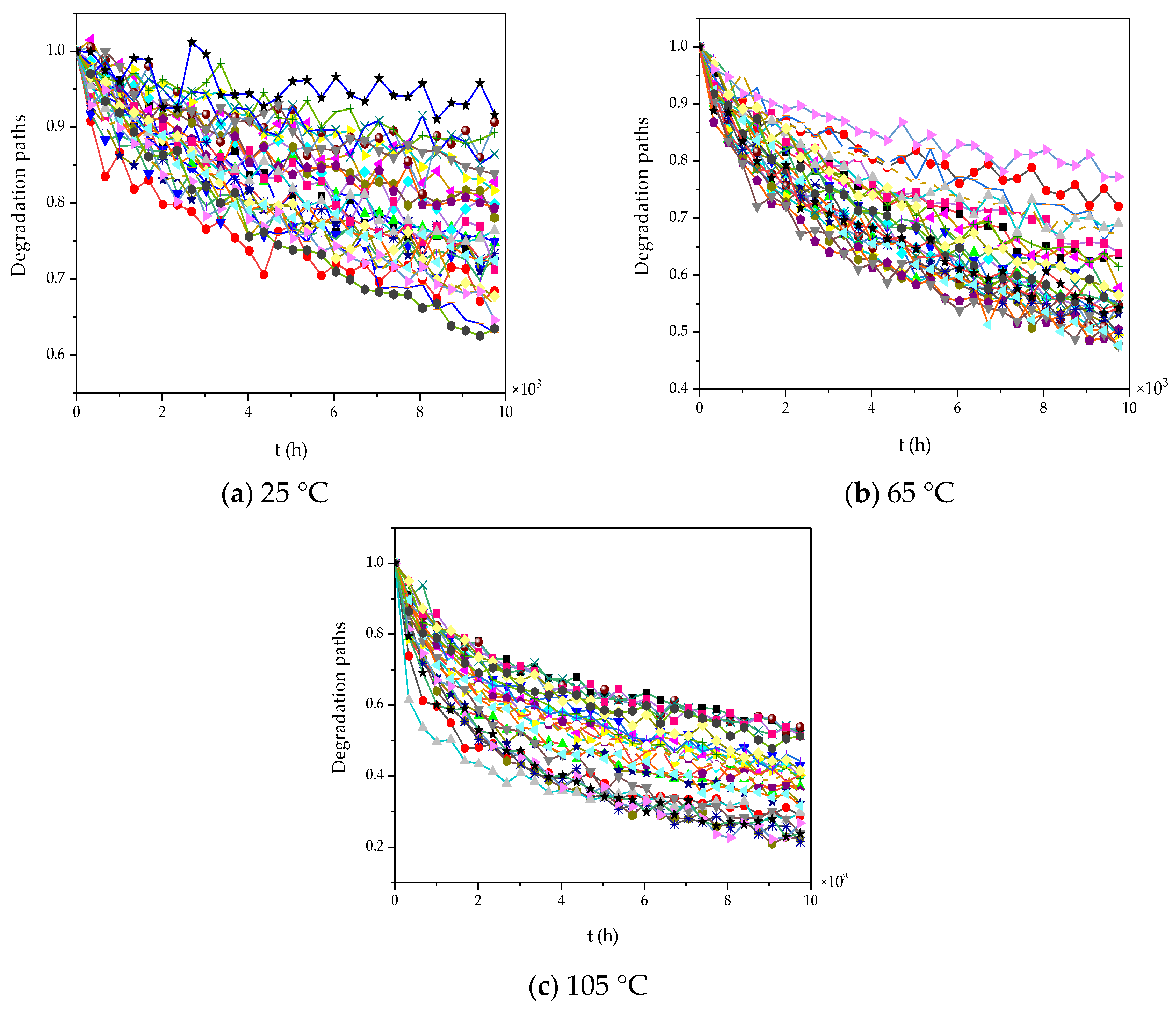
4.1. Model Verification

To demonstrate the effectiveness and applicability of the above model, this section compares some degradation methods with an illustrative example. For simplicity, the proposed model in this paper in Equation (17) is referred to as $M_0$.

$$M_0:Y\left(t|S_k\right)={\lambda }_k\mathrm{\Lambda }\left(t\right)+{\left({\sigma }_B\right)}_{k}B\left(\mathrm{\Lambda }\left(t\right)\right)+{\sigma }_{\epsilon }\epsilon$$

(29)

where ${\lambda }_k=\eta \exp \left(-b/S_k\right)$, $\eta \sim N\left({\mu }_{\eta },{\sigma }_{\eta }^2\right)$, ${\left({\sigma }_B^2\right)}_k=\kappa {\varsigma }_k$, ${\sigma }_{\epsilon }\epsilon \sim N\left(0,{\sigma }_{{}^{\epsilon }}^2\right)$.

If the acceleration factor constant principle is not considered, then $M_0$ becomes a nonlinear Wiener process model whose diffusion parameter ${\sigma }_B$ is fixed that has no relationship with the applied stress, which is referred to $M_1$.

$$M_1:Y\left(t|S_k\right)={\lambda }_k\mathrm{\Lambda }\left(t\right)+{\left({\sigma }_B\right)}_{k}B\left(\mathrm{\Lambda }\left(t\right)\right)+{\sigma }_{\epsilon }\epsilon$$

(30)

where ${\lambda }_k=\eta \exp \left(-b/S_k\right)$, $\eta \sim N\left({\mu }_{\eta },{\sigma }_{\eta }^2\right)$, ${\sigma }_{\epsilon }\epsilon \sim N\left(0,{\sigma }_{{}^{\epsilon }}^2\right)$.

If the measurement errors are not considered, then $M_0$ becomes a nonlinear Wiener process model without measurement errors which is referred to $M_2$.

$$M_2:Y\left(t|S_k\right)={\lambda }_k\mathrm{\Lambda }\left(t\right)+{\left({\sigma }_B\right)}_{k}B\left(\mathrm{\Lambda }\left(t\right)\right)$$

(31)

where ${\lambda }_k=\eta \exp \left(-b/S_k\right)$, $\eta \sim N\left({\mu }_{\eta },{\sigma }_{\eta }^2\right)$.

The fits of these different Wiener process models were compared by the Akaike Information Criterion (AIC). AIC handles the trade-off between the goodness of model fit and the complexity of the model, which is defined as

$$AIC=2m-2\ell$$

(32)

In Equation (32), the number of unknown parameters is $m$ and the maximized value of the log-likelihood function of the estimated model is $\ell$. The model with the lowest AIC values in several potential models would be selected as the best-fit one.

Taking the example of the constant accelerated degradation data of light-emitting diodes (LED) in [26], the data contain three accelerated levels of thermal stress, 25 °C, 65 °C, and 105 °C. At each accelerated thermal stress, there were 25 LEDs whose light intensity was recorded at 29 inspection times. Supposing the initial value is 1, LED fails when the relative luminosity drops to 0.5. Thus, 50% of the initial luminosity is the failure threshold. The degradation paths of light intensity of LEDs are shown in Figure 1.

According to the degradation trajectory of the 75 LEDs, let $\mathrm{\Lambda }\left(t\right)=t^{0.5}$ for simplicity. The degradation results of LEDs mentioned above are listed in

Table 2. Comparisons of three different degradation models with LEDs CSADT degradation data.

	${\widehat{\mathit{\mu }}}_{\mathit{\eta }}$	${\widehat{\mathit{\sigma }}}_{\mathit{\eta }}$	$\widehat{\mathit{b}}$	$\mathit{\kappa }$	${\widehat{\mathit{\sigma }}}_{\mathit{B}}$	${\widehat{\mathit{\sigma }}}_{\mathit{\epsilon }}$	$\mathit{\ell }$	$\mathit{A}\mathit{I}\mathit{C}$
$M_0$	1.0223	0.2915	1934.6	0.032	/	0.036	4511.7	−9011.4
$M_1$	1.2889	0.3120	1831.7	/	0.0071	0.027	4241.6	−8473.2
$M_2$	1.3781	0.0001	1853.1	/	0.026	/	3691.2	−7374.4

after comparing the applicability of different models mentioned above, and we can find that the model $M_0$ has the lowest $AIC$ and the highest $\ell$ compared with other models. It shows that the raised model in this paper has a better model goodness-of-fit than the others.

Thus, it is necessary to consider the nonlinearity, acceleration factor constant principle, unit-to-unit variability, and measurement errors when modeling the degradation paths.

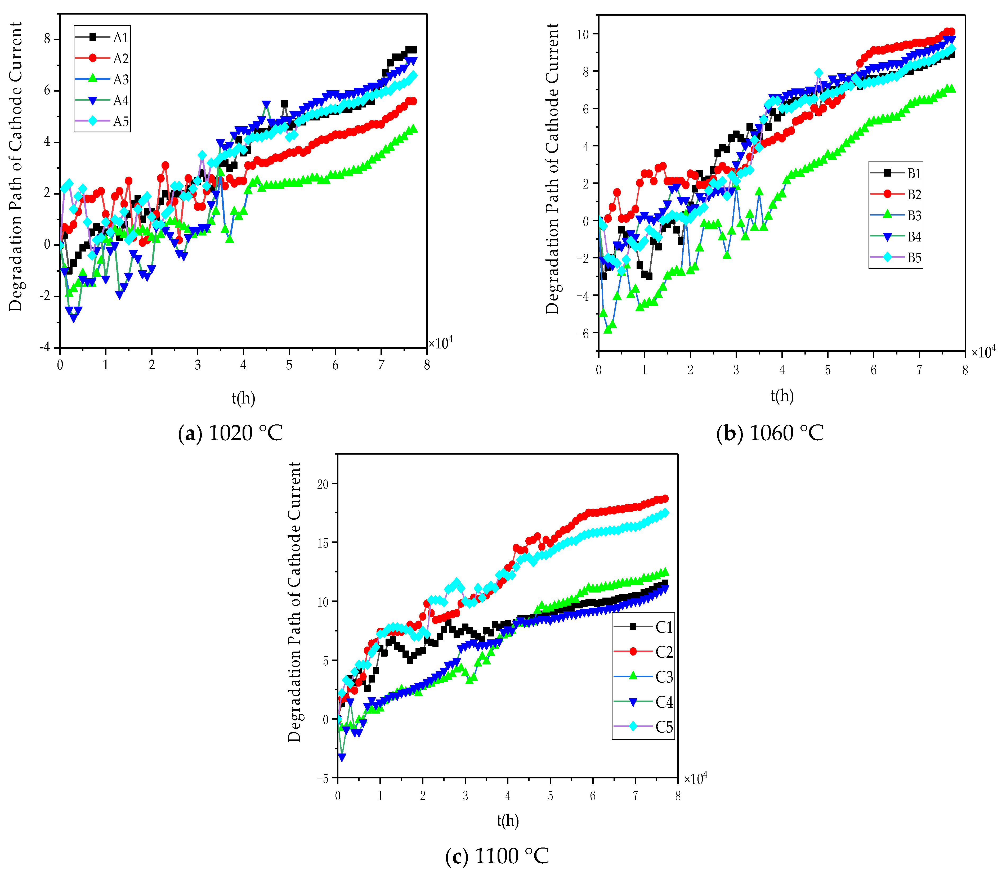
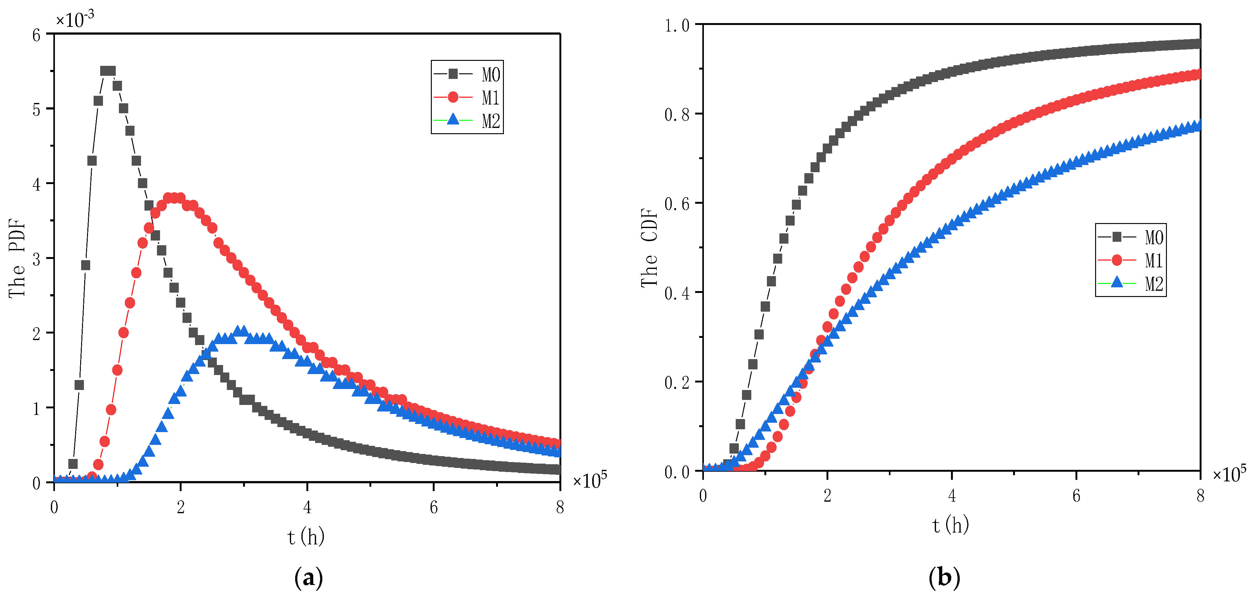
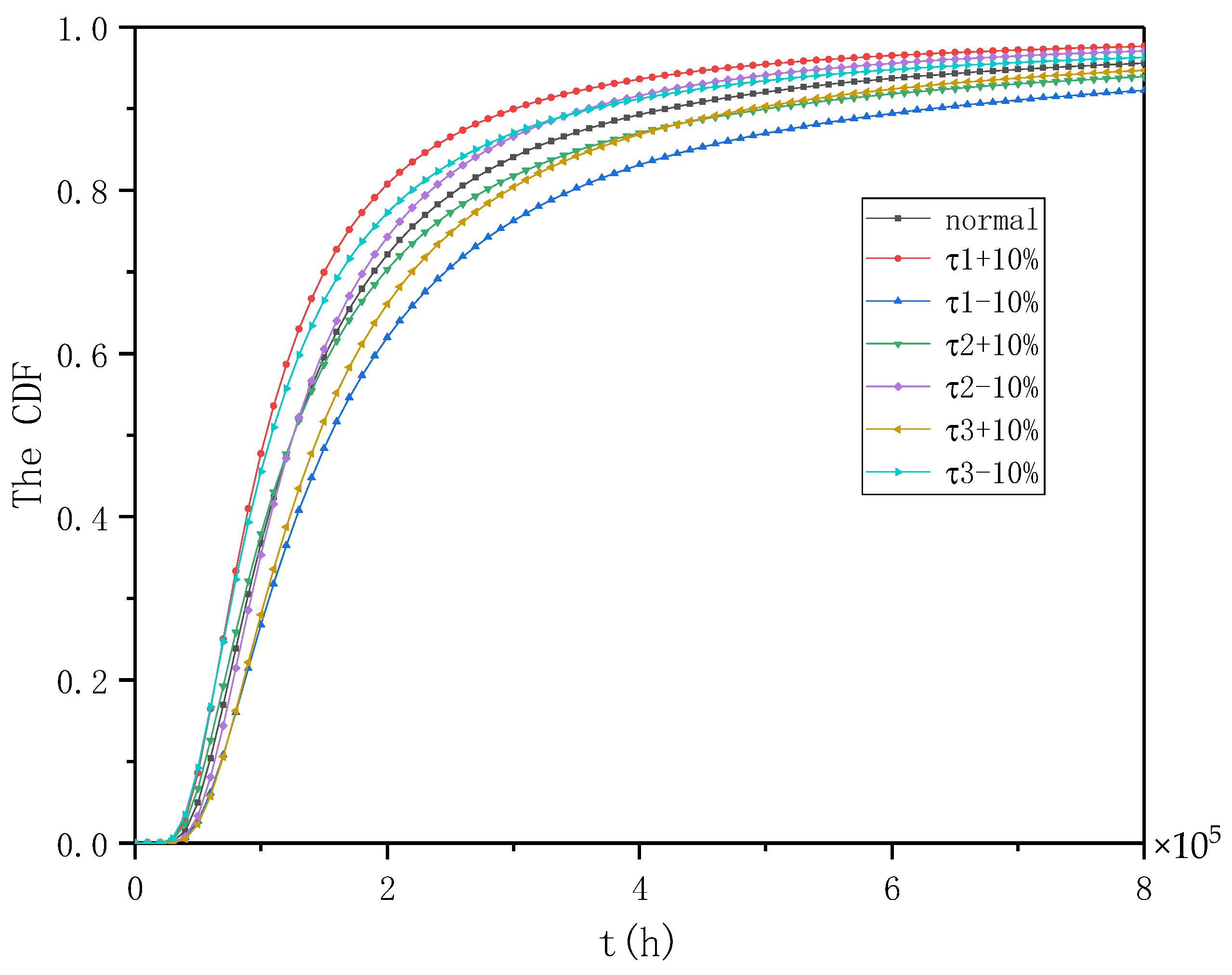
4.2. Case Application and Sensitivity Analysis

TWT has the merit of high reliability, long lifetime, high gain, and large power which is one of the most extensively used vacuum electronic devices [27], thus it is widely applied in the area of aerospace. TWT mainly consists of an electronic gun, slow-wave structure, RF input and output, permanent magnet and collector [28]. The cathode is an important part of the electron gun, which determines the life of TWTs under good vacuum conditions [29], and it is called the heart of TWT. The CSADT for TWTs is carried out under three temperature levels: 1020 °C, 1060 °C, and 1100 °C. The normal operational level is 980 °C. Five cathodes are put to the test at three stress levels and the degradation data are recorded every 1000 h until 77,000 h. The emission current of a cathode decreases over time, causing a soft failure when its emission current drops below a critical failure threshold.

The performance degradation $\Delta \mathrm{y}$ is the change of cathode emission current $y$ relative to the initial value $y_0$ at a certain time. However, the cathode emission current decreases gradually with time, for the sake of ensuring that the degradation process of the cathode is a positive drift, that is, the drift parameter is positive, the performance degradation takes the decreased value of the cathode emission current at a certain moment relative to the initial value. That is, $\Delta \mathrm{y}=y_0-y$. Therefore, the failure threshold is positive. The cathode is considered to have failed when the relative degradation value of the emission current exceeds 10% of the initial emission current whose failure threshold is $D=13$ [30]. The degradation paths of the fifteen tested units under three stress levels are described in Figure 2, showing that the degradation of samples uniformly exhibits a nonlinear characteristic especially at the beginning of the CSADT. Thus, the degradation process is modeled with a time-scale transformed Wiener process as Equation (17) with $\mathrm{\Lambda }\left(t\right)=t^{\theta }$, which lets $\theta =0.5$ for simplicity according to the degradation trajectory.

According to [29], the degradation rate of cathodes at a constant emission current can be described by the Arrhenius model. Therefore, we use a stochastic Arrhenius model to represent the acceleration model applied to determine the relationship between the failure time data and the working temperature stress. Based on the parameters estimation method proposed in Section 3, we can obtain the estimation results of parameters and the $AIC$ as shown in

Table 3. The parameters of three degradation models with TWT CSADT degradation data.

	${\widehat{\mathit{\mu }}}_{\mathit{\eta }}$	${\widehat{\mathit{\sigma }}}_{\mathit{\eta }}$	$\widehat{\mathit{b}}$	$\mathit{\kappa }$	${\widehat{\mathit{\sigma }}}_{\mathit{B}}$	${\widehat{\mathit{\sigma }}}_{\mathit{\epsilon }}$	$\mathit{\ell }$	$\mathit{A}\mathit{I}\mathit{C}$	$\mathit{M}\mathit{T}\mathit{T}\mathit{F}$
$M_0$	0.1092	0.0387	932	0.000020	/	0.00268	2146.9	−4283.8	25.34 a
$M_1$	0.0923	0.0316	1200	/	0.034	0.00951	1976.4	−3942.8	27.48 a
$M_2$	0.1281	0.03	1678	/	0.29	/	1389.7	−2771.4	28.28 a

a—annual.

, indicating that $M_0$ clearly outperforms other models in terms of $AIC$. It is shown that the proposed model has a better fit than the others.

In Figure 3, we describe the PDF and CDF under the normal operating temperature $T_0=980℃$ based on the parameter estimation results presented in Table 3. The time corresponding to the peak values of PDF were as follows: 0.0055, 0.0038, and 0.002 for $M_0$ to $M_2$, respectively. However, the $MTTF$ of $M_0$ is the smallest from Table 3, which is 25.34 a, and it is more close to the actual engineering due to the uncertainties and acceleration factor constant principle compared to other models.

In engineering applications, the estimated parameter $\widehat{\mathsf{\Theta }}=\left\{\widehat{{\mu }_{\eta }},\widehat{{\sigma }_{\eta }^2},\widehat{\kappa },\widehat{b},\widehat{{\sigma }_{\epsilon }^2}\right\}$ in $M_0$ would deviate from the true parameter $\mathsf{\Theta }=\left\{{\mu }_{\eta },{\sigma }_{\eta }^2,\kappa ,b,{\sigma }_{\epsilon }^2\right\}$. Thus, it is necessary to do sensitivity analysis because it reflects the degree to which the output value of the model changes with small changes in parameters. Without loss of generality, we assume ${\tau }_1$, ${\tau }_2$, and ${\tau }_3$ represent the bias of parameters ${\mu }_{\eta },{\sigma }_{\eta }^2,b$, respectively (because the values of $\kappa$ and ${\sigma }_{\epsilon }^2$ are too small, we do not consider their errors). Based on Equation (15), when the bias range of the parameter is ±10%, sensitivity analysis of the reliability of cathode on threshold $D=13$ is presented in Figure 4. From these results, we can find that the model $M_0$ tends to be robust, and the range of ${\mu }_{\eta }$ is more sensitive to the output value than the others. Therefore, more attention of ${\mu }_{\eta }$ should be paid to the process of optimization.

5. Conclusions

In this paper, a degradation model based on a nonlinear Wiener process was developed for constant stress-accelerated degradation data. Before establishment, the relation between the drift parameter and diffusion parameter was derived from the accelerated factor constant principle, and their relation to the stress variable was deduced. Moreover, to represent the unit-to-unit variability among different individuals during accelerated degradation processes, random effects were also considered when the drift parameter was assumed to be a normal distribution and the diffusion parameter was set as a constant under certain stress. The degradation path considering the measurement error was modeled using the degradation data in CSADT, and the unknown parameters were solved with MLE based on the properties of the Wiener process. Finally, the superiority of the existing model was demonstrated with engineering comparison under the same conditions.

The innovation of this paper lies in the following: Firstly, the relation between the drift parameter and diffusion parameter was deduced by the acceleration factor constant principle. Secondly, the uncertainties were considered such as random effects, nonlinear, and measurement errors. Thirdly, the unknown parameters were solved with the MLE method by applying a multi-dimensional search whose initial value was confirmed by the least square method. Last but not least, an innovative application to the TWT was conducted which was the first time to assess lifetime by using degradation data.

However, much work is still needed to study the method of modeling because we only considered some of the uncertainties and the degradation data. Further research may study the model of multi-information infusion and the method of estimating the unknown parameter.

References

1. Meeker, W.Q.; Escobar, L.A. Accelerated degradation tests: Modeling and analysis. Technometrics 1998, 40, 89–99. [Google Scholar] [CrossRef]
2. Lu, C.; Meeker, W. Using degradation measures to estimate a time-to -failure distribution. Technometrics 1993, 35, 161–174. [Google Scholar] [CrossRef]
3. Tang, S.; Guo, X.; Yu, C.; Xue, H.; Zhou, Z. Accelerated degradation tests modeling based on the nonlinear Wiener process with random effect. Math. Probl. Eng. 2014, 2014, 560726. [Google Scholar] [CrossRef]
4. Onar, A.; Padgett, W.J. Acceleratedtest models with the inverse Gaussian distribution. J. Stat. Plan. Inference 2000, 89, 119–133. [Google Scholar] [CrossRef]
5. Tsai, T.-R.; Lio, Y.L.; Jiang, N. Optimal decisions on the accelerated degradation test plan under the Wiener process. Qual. Technol. Quant. Manag. 2014, 11, 461–470. [Google Scholar] [CrossRef]
6. Ye, Z.-S.; Xie, M. Stochastic modeling and analysis of degradation for highly reliable products. Appl. Stoch. Models Bus. Ind. 2015, 31, 16–32. [Google Scholar] [CrossRef]
7. Tang, L.C.; Yang, G.; Xie, M. Planning of step-stress accelerated degradation test. In Proceedings of the Annual Symposium Reliability and Maintainability, 2004-RAMS, Los Angeles, CA, USA, 26–29 January 2004; pp. 287–292. [Google Scholar]
8. Wang, X.; Balakrishman, N.; Guo, B. Residual life estimation based on a generalized Wiener degradation process. Reliab. Eng. Syst. Saf. 2014, 124, 13–23. [Google Scholar] [CrossRef]
9. Wang, X.; Jiang, P.; Guo, B.; Cheng, Z. Real-time reliability evaluation with a general Wiener process-based degradation model. Qual. Reliab. Eng. Int. 2014, 30, 205–220. [Google Scholar] [CrossRef]
10. Ye, Z.S.; Chen, N.; Shen, Y. A new class of Wiener process models for degradation analysis. Reliab. Eng. Syst. Saf. 2013, 112, 38–47. [Google Scholar] [CrossRef]
11. Park, C.; Padgett, W.J. Accelerated degradation models for failure based on geometric Brownian motion and gamma processes. Lifetime Data Anal. 2005, 11, 511–527. [Google Scholar] [CrossRef]
12. Wang, L.; Pan, R.; Li, X.; Jiang, T. A Bayesian reliability sevalution method with integrated accelerated degradation testing and field information. Reliab. Eng. Syst. Saf. 2013, 112, 38–47. [Google Scholar] [CrossRef]
13. Liao, H.T.; Elsayed, E.A. Reliability inference for field conditions from accelerated degradation testing. Nav. Res. Logist. 2006, 53, 576–587. [Google Scholar] [CrossRef]
14. Whitmore, G.A.; Schenkelberg, F. Modeling accelerated degradation data using Wiener diffusion with A time scale transformation. Lifetime Data Anal. 1997, 3, 27–45. [Google Scholar] [CrossRef]
15. Tang, S. Step stress accelerated degradation process modeling and remaining useful life estimation. J. Mech. Eng. 2014, 50, 16–33. [Google Scholar] [CrossRef]
16. Chen, Z.; Li, S.; Pan, E. Optimal Constant-Stress Accelerated Degradation Test Plans Using Nonlinear Generalized Wiener Process. Math. Probl. Eng. 2016, 2016, 9283295. [Google Scholar] [CrossRef]
17. Peng, C.Y.; Tseng, S.T. Mis-specification analysis of linear degradation models. IEEE Trans. Reliab. 2009, 58, 444–455. [Google Scholar] [CrossRef]
18. Si, X.S.; Wang, W.; Hu, C.H.; Zhou, D.H.; Pecht, M.G. Remaining useful life estimation based on a nonlinear diffusion degradation process. IEEE Trans. Reliab. 2012, 61, 50–67. [Google Scholar] [CrossRef]
19. Si, X.S.; Wang, W.; Hu, C.H.; Chen, M.Y.; Zhou, D.H. A Wiener–Process-based degradation model with a recursive filter algorithm for remaining useful life estimation. Mech. Syst. Signal Process. 2013, 35, 219–237. [Google Scholar] [CrossRef]
20. Tsai, C.C.; Tseng, S.T. Mis-specification analyses of gamma and Wiener degradation processes. J. Stat. Plan. Inference 2011, 11, 3725–3735. [Google Scholar] [CrossRef]
21. Pieruschka, E. Relation between Lifetime Distribution and the Stress Level Causing Failure; Lockheed Missiles and Space Division: Sunnyvale, CA, USA, 1961. [Google Scholar]
22. Nelson, W.B. Accelerated Testing: Statistical Models, Test Plans, and Data Analysis; John Wiley & Sons: Hoboken, NJ, USA, 2009. [Google Scholar]
23. Wang, H.W.; Teng, K.N.; Zhou, Y. Design an optimal accelerated-stress reliability acceptance test plan based on acceleration factor. IEEE Trans. Reliab. 2018, 67, 1008–1018. [Google Scholar] [CrossRef]
24. Zhang, Z.X.; Si, X.S.; Hu, C.H.; Zhang, Q.; Li, T.M.; Xu, C.Q. Planning repeated degradation testing for products with three-source variability. IEEE Trans. Reliab. 2016, 65, 640–647. [Google Scholar] [CrossRef]
25. Wang, H.W.; Teng, F. Accelerated Degradation Data Modeling and Statistical Analysis Methods and Engineering Applications; Science Press: Beijing, China, 2020. [Google Scholar]
26. Hamada, M.S.; Wilson, A.; Reese, C.S. Bayesian Reliability; Springer: Berlin, Germany, 2008. [Google Scholar]
27. Sharma, R.K.; Choudhury, A.R.; Arya, S.; Ghosh, S.K.; Srivastava, V. Design and Experimental Evaluation of Dual-Anode Electron Gun and PPM Focusing of Helix TWT. IEEE Trans. Electron Devices 2015, 62, 3419–3425. [Google Scholar] [CrossRef]
28. Zhang, M.; Liu, Y.W.; Yu, S.; Wang, Y.; Zhang, H. Life Test Studies on Dispenser Cathode with Dual-Layer Porous Tungsten. IEEE Trans. Electron Devices 2014, 61, 2983–2988. [Google Scholar] [CrossRef]
29. Ishibori, K.; Mita, N.; Yamamoto, K. A 10 W, 20 GHz-band traveling-wave tube amplifier for communications satellite. Rev. Electr. Commun. Lab. 1983, 31, 634–641. [Google Scholar]
30. Feltham, S.J.; Kornfeld, G.; Lotthammer, R.; Stevenson, J.L. Life test studies on MM-cathodes. IEEE Trans. Electron Devices 1990, 37, 2558–2563. [Google Scholar] [CrossRef]
Figure 1. The degradation trajectory of LEDs under CSADT over time t at (a) 25 °C, (b) 65 °C, (c) 105 °C.
Applsci 11 08968 g001
Figure 2. Degradation trajectory of cathode emission current at (a) 1020 °C, (b) 1060 °C, (c) 1100 °C.
Applsci 11 08968 g002
Figure 3. The comparison of the PDF and CDF of the three models for TWT CSADT data (a) PDF, (b) CDF.
Applsci 11 08968 g003
Figure 4. Sensitivity analysis of M 0 with a fluctuation range of ±10%.
Applsci 11 08968 g004