Abstract
Conventional fractional open-circuit voltage (FOCV) methods in maximum power point tracking (MPPT) are widely adopted for their simple structure and low computing power requirements. However, under mismatch and environmental changing conditions, the FOCV methods introduce a large amount of energy loss due to their maximum power point being fixed at the initial setup. To reduce energy loss, the intermittent FOCV MPPT proposed in this paper regularly refreshes all the parameters for each condition in time by using an I-V curve tracer. The proposed intermittent FOCV consists of two phases: the scan and set phases. In scan phase, the I-V curve of a photovoltaic (PV) cell is scanned and its power is calculated. In set phase, the global MPP of the PV cell is extracted and set by controlling the 8-bit capacitance array. Simulation and calculation based on experimental results with a single PV cell show that the energy loss of the proposed intermittent FOCV under daily temperature and illuminance distributions decreased by up to 99.9% compared to that of the conventional FOCV.
1. Introduction
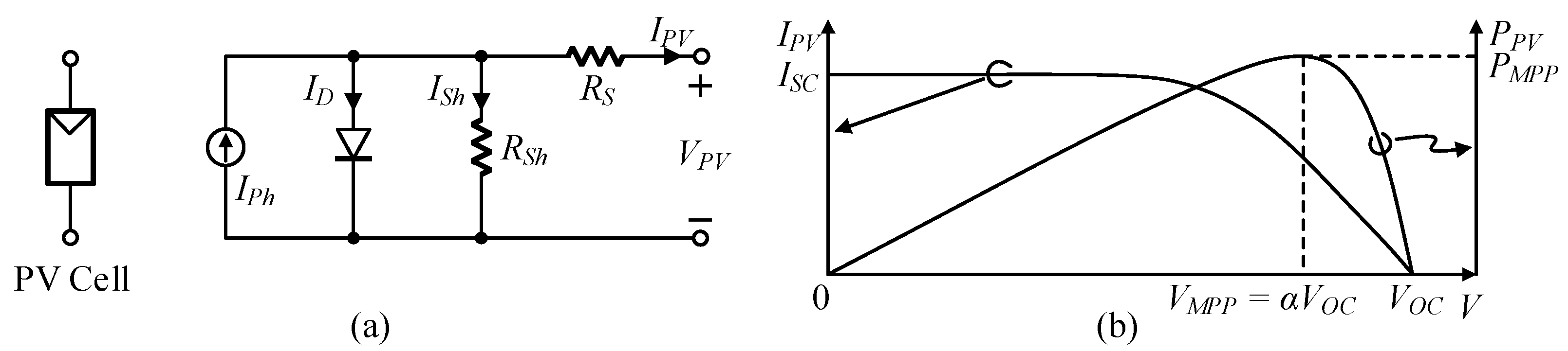
Batteryless Internet-of-Things (IoT) devices have been widely used for various wireless sensors by converting light [1], vibration [2,3], and thermal gradient [4] into electric energy. Among these various sources, a photovoltaic (PV) cell that harvests electric energy from light is the most anticipated energy source [1,5]. Since the performance and I-V characteristics of the PV cell vary depending on external environmental factors such as irradiance, temperature, and load impedance, maximum power point tracking (MPPT) methods are necessary for maximizing the power output of PV cells under various conditions [6]. Figure 1a shows an electrical model of a PV cell. Sweeping the voltage of the PV cell, , the current, , and the power, can be obtained as Figure 1b [7]. The MPP can be determined at the voltage , where is linear factor.
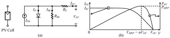
Figure 1.
PV cell: (a) Electrical model and (b) I-V and P-V characteristics of a PV cell.
There have been many MPPT methods: single step algorithm including perturb & observe (P & O), binary-weighted step algorithm including successive approximation register (SAR) [8], combined algorithm based on adaptively binary-weighted step (ABWS) and monotonically decreased step (MDS) [8], and fractional open-circuit voltage (FOCV) [9,10,11,12]. The P & O method is very popular method due to its flexibility and balance between complexity and accuracy. It can also dynamically detect the actual MPP with high tracking efficiency, although at the expense of oscillation around the MPP at the steady state, which causes a large amount of energy loss [12,13,14]. Therefore, the P & O technique is not appropriate for low power and low energy environments. SAR MPPT technique is based on the binary-weighted step (BWS) for fast tracking [13], but the most-significant-bit (MSB) operation runs first in the SAR MPPT, which aggravates the overall energy loss [6]. Although least-significant-bit (LSB) switching at the initial step in [8] reduces abrupt energy loss, a large amount of power consumption for calculating PV power makes this method improper for low energy environments. Furthermore, the three aforementioned methods cannot detect the global MPP (GMPP), so that they are not appropriate for PV cells with multiple MPPs.
As depicted in Figure 1b, in an FOCV method, the MPP is determined at the fraction of the open-circuit voltage of a PV cell, . For a simple structure and low power consumption, the FOCV methods adopt approximation-based techniques that are a more appropriate method for low energy environments [8]. However, if changes in environmental conditions are present, the mismatch of between the new and the previous values by the FOCV leads to a large amount of energy loss. In this paper, while taking advantage of FOCV methods, the GMPP is regularly scanned by using an I-V curve tracer, and the re-evaluated is set for MPPT without using an additional ad-hoc parameter.
2. Conventional MPPT Algorithms
2.1. Perturb and Observe (P & O)
The procedure to track the MPP in the P & O algorithm is explained as follows: the P & O algorithm operates by periodically incrementing or decrementing the voltage of a PV cell. At first, the MPPT controller measures the voltage and the current of the PV cell. Then, the present power is compared to the previous power of the PV cell. Depending on whether the present power or the previous power is larger, the controller changes the PV voltage. If the present power is higher than the previous power, the P & O algorithm keeps increasing the input voltage of the PV cell, and vice versa. It is very simple to implement, but it is not appropriate for low power and low energy environments because of overall power loss caused by the fluctuation of its operating point around the MPP. If there are multiple MPPs, it cannot detect the GMPP because of the oscillation.
2.2. Successive Approximate Register (SAR)
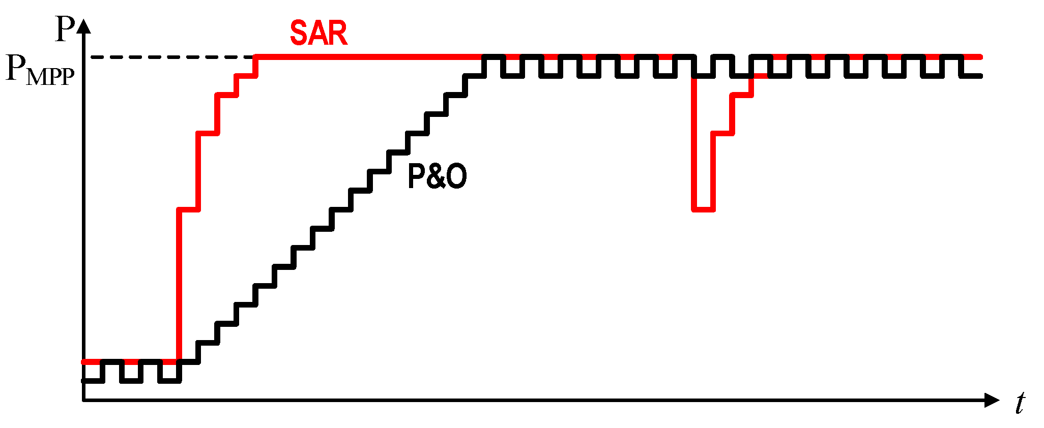
The SAR MPPT includes an active mode and a power down mode that alternate periodically [6]. The SAR MPPT tracks the MPP in the active mode, and maintains the final voltage of the previous active mode during the power down mode. Unlike the P & O algorithm that tracks the MPP with a single step, the SAR MPPT uses the BWS to make the tracking speed faster than the P & O. Therefore, like the P & O, it is not appropriate for low power and low energy environments. Figure 2 shows the MPP tracking procedure of the conventional P & O and the SAR over time.
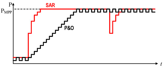
Figure 2.
The MPP tracking procedure of the conventional P & O and the SAR over time.
2.3. Combined Algorithm Based on the Adaptively Binary-Weighted Search (ABWS) and the Monotonically Decreased Step (MDS)
The combined algorithm based on the adaptively binary-weighted search (ABWS) and the monotonically decreased step (MDS) aims at tracking the MPP as quickly as possible in order to reduce the power loss under rapidly changing environmental conditions [8]. Similar to the BWS, the ABWS tracks the MPP by increasing the voltage step, but starts from the LSB until the operating voltage step passes the MPP. Then, the ABWS stops and the MDS starts to operate, tracking the exact MPP. The MDS monotonically reduces the voltage step until the MPP is found. If the variation of the MPP drops below 1 LSB resolution, the MPP remains unchanged and the MDS operation is finished. Compared to the P & O and the SAR, this algorithm tracks the MPP faster than the P & O and consumes less power under stable environments.
2.4. Fractional Open-Circuit Voltage (FOCV)
The main principle of this technique comes from the relationship between the voltage of maximum power-point () and the open-circuit voltage (), which the approximately equals to some fractional value of the . The relationship between the two voltages is defined as
where is the linear factor. Since there is no procedure for tracking the MPP, the FOCV method features the lowest implementation complexity and consumes the lowest circuit power. Therefore, the FOCV method is the most appropriate method for low-power and low-energy devices. Figure 3 illustrates the comparison of the circuit power consumption over time and the power consumption for the given time between the P & O, the SAR, and the FOCV algorithm.
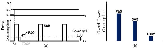
Figure 3.
Comparison of (a) the power consumption for MPPT in time (b) the energy loss between the P & O, the SAR, and the FOCV algorithms for the given time.
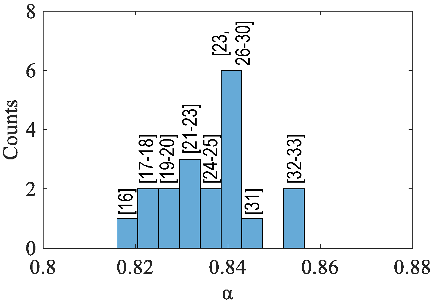
However, the MPP of the FOCV method is not the real MPP, but the approximated value. In [15], it is insisted that can be located within the range from 0.71 to 0.78. However, the values of recent PV cells on the market can be easily found between 0.8 and 0.86, as shown in Figure 4, which shows the histogram of distribution of the values for PV cells in [16,17,18,19,20,21,22,23,24,25,26,27,28,29,30,31,32,33]. Therefore, it is essential to set the exact and the MPP because values are distributed in a wide range for each PV cell.
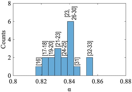
Figure 4.
Histogram of distribution of the value.
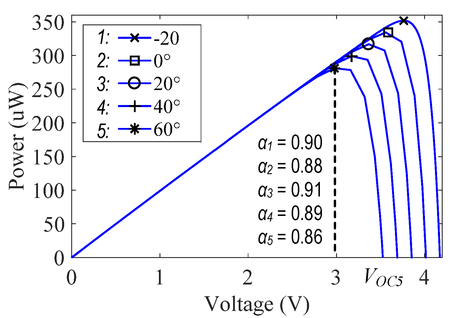
Furthermore, if external environmental factors like illuminance and temperature cause changes in the MPP, energy loss can potentially happen unless the previous value of is reset to new . Figure 5 shows how the P-V characteristics and the of a PV cell that has the value of 0.88 at 27 °C vary depending on temperature.

Figure 5.
Power versus voltage characteristics of a PV cell and the change of the value of under various temperature conditions.
If and the MPP are not reset as soon as possible, the energy loss increases. To reduce the energy loss caused by unreal MPP, the proposed FOCV intermittently and dynamically scans the I-V curve of the PV cell to detect the GMPP and reset the and the MPP. Although the circuit power consumption caused by dynamically scanning and resetting the MPP can be larger than the P & O and SAR, it operates intermittently, so that the total energy loss of the proposed FOCV is much lower than that of the P & O, SAR, and conventional FOCV. Figure 6 illustrates the comparison of the energy loss between the conventional and the proposed FOCV under varying conditions.
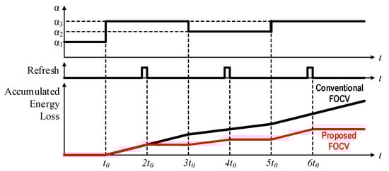
Figure 6.
Comparison of the accumulated energy loss between the conventional and the proposed FOCV with refreshing frequency of under varying .
3. Proposed FOCV MPPT Algorithm
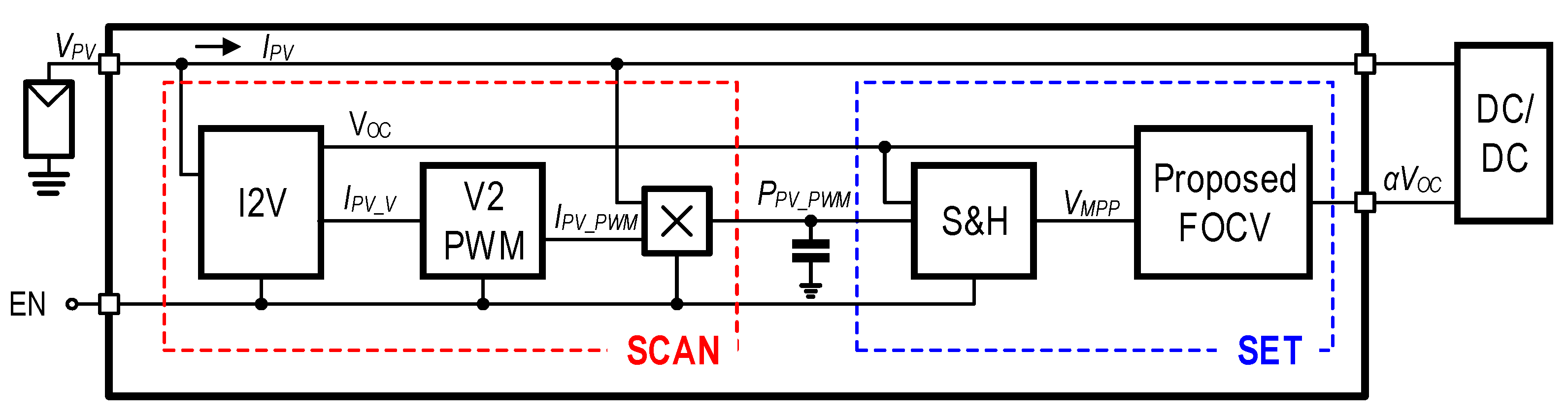
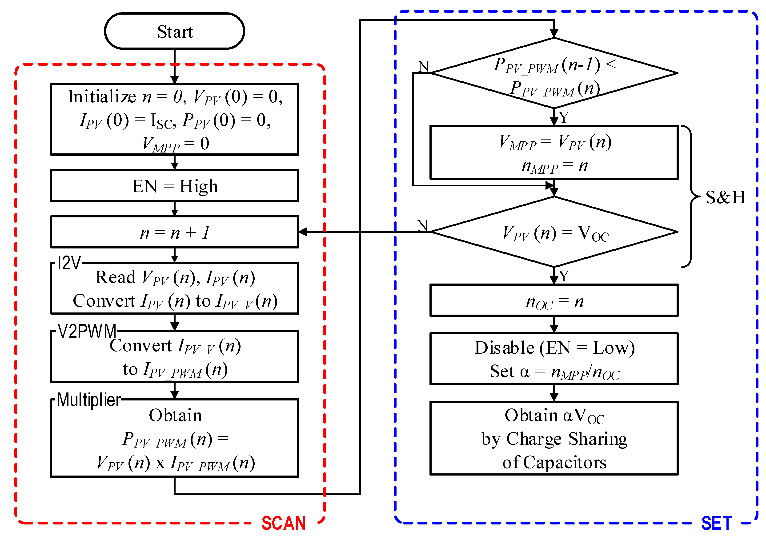
Unlike conventional MPPT methods, the proposed MPPT method finds GMPP because it scans the I-V curve for its working voltage range regardless of the number of local MPPs. The block diagram of the proposed FOCV MPPT circuit using an I-V curve tracer is shown in Figure 7 and the flow chart of the proposed FOCV MPPT is shown in Figure 8. The proposed FOCV MPPT technique consists of two phases, scan and set. In the first phase, also called scan phase, the system scans the voltage and current and calculates the power of the PV cell with the current-to-voltage converter (I2V), the voltage-to-PWM converter (V2PWM), and the multiplier. In the second phase, also called set phase, the system sets the MPP and with the calculated value of the scan phase. Set phase consists of the sample and hold (S & H), and the proposed FOCV circuit.
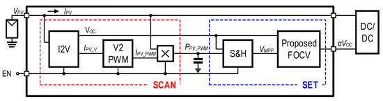
Figure 7.
The block diagram of the proposed FOCV MPPT using an I-V curve tracer.
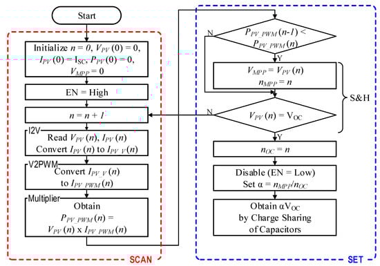
Figure 8.
The flow chart of the proposed FOCV MPPT using an I-V curve tracer.
3.1. Scan Phase
3.1.1. Current-To-Voltage (I2V) Converter and Voltage-To-PWM (V2PWM) Converter
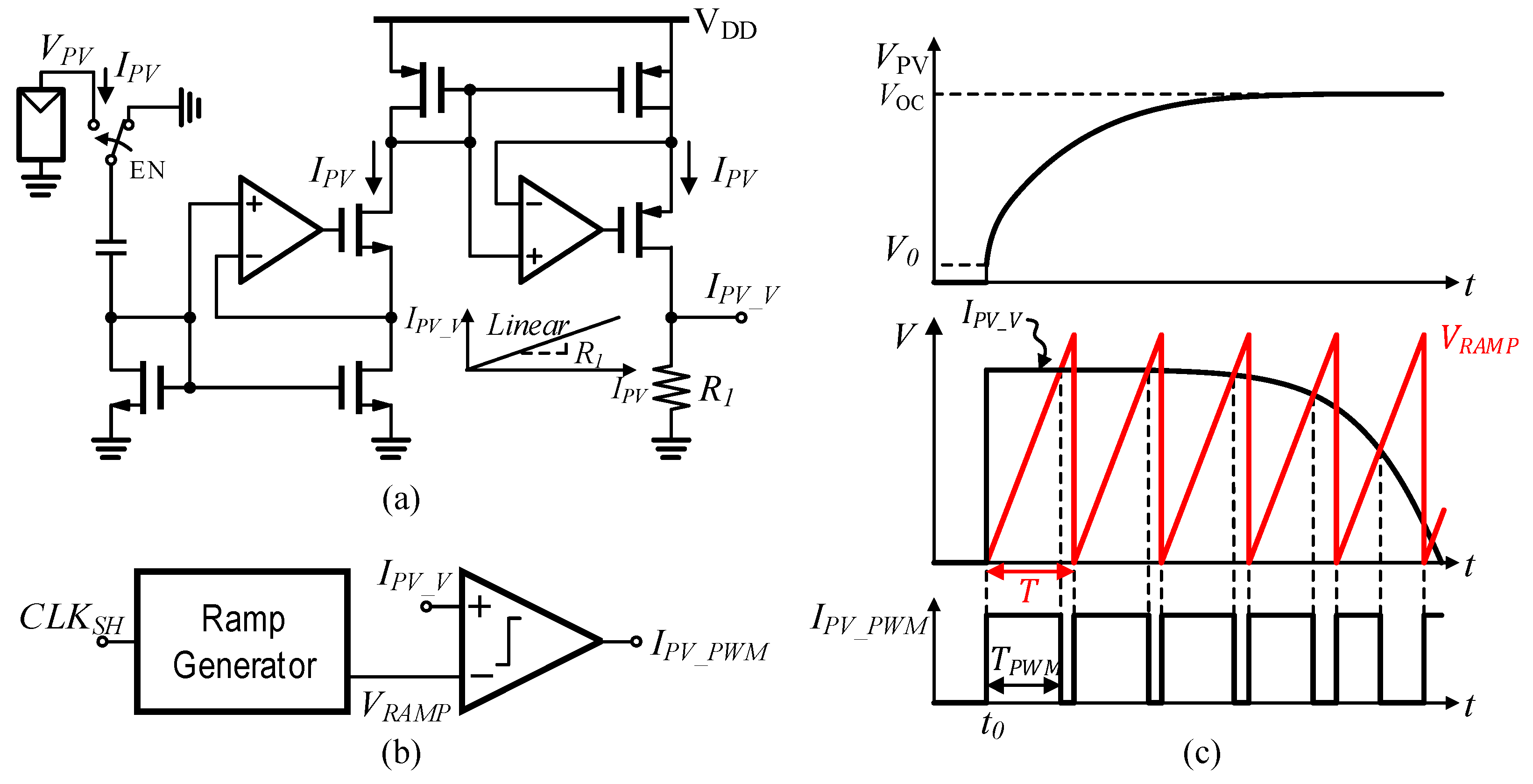
Figure 9 shows the block diagrams of the proposed I2V converter and the proposed V2PWM converter, and the timing diagrams of the I2V and the V2PWM. The I2V converter that uses the current mirror technique sweeps and scans the voltage and the current of a PV cell and makes the I-V curve. Once the enable signal () is high and the switch between the PV cell and the I2V converter turns on, the I2V sweeps and scans the current of the PV cell () from the short-circuit current () to , and the voltage of the PV cell () from to . At the same time, , which is mirrored by two current mirrors, is converted into voltage form () by being multiplied with a resistor, . The relation between and can be expressed as
where is the number of iterations. For better linearity, two OP AMPs are implemented in the I2V by making each of MOSFET that is connected to the input of OP AMP the same.

Figure 9.
The block diagrams of (a) the current-to-voltage (I2V) converter and (b) the voltage-to-PWM (V2PWM) converter and (c) the timing diagrams of the I2V converter and the V2PWM converter.
The V2PWM converter is composed of two circuits, a ramp generator and a comparator. The ramp generator generates a ramp signal () whose peak voltage () is higher than the maximum value of , . Comparing with , the comparator generates the PWM duty signal, . Using the constancy of the slope of , the slope can be expressed as
where is the period of the ramp signal and is the width of the duty signal of each iteration. Therefore, can be expressed as Equation (4).
As shown in Equation (4) and Figure 9c, the higher the current is, the wider the width of the duty signal is.
3.1.2. Multiplier
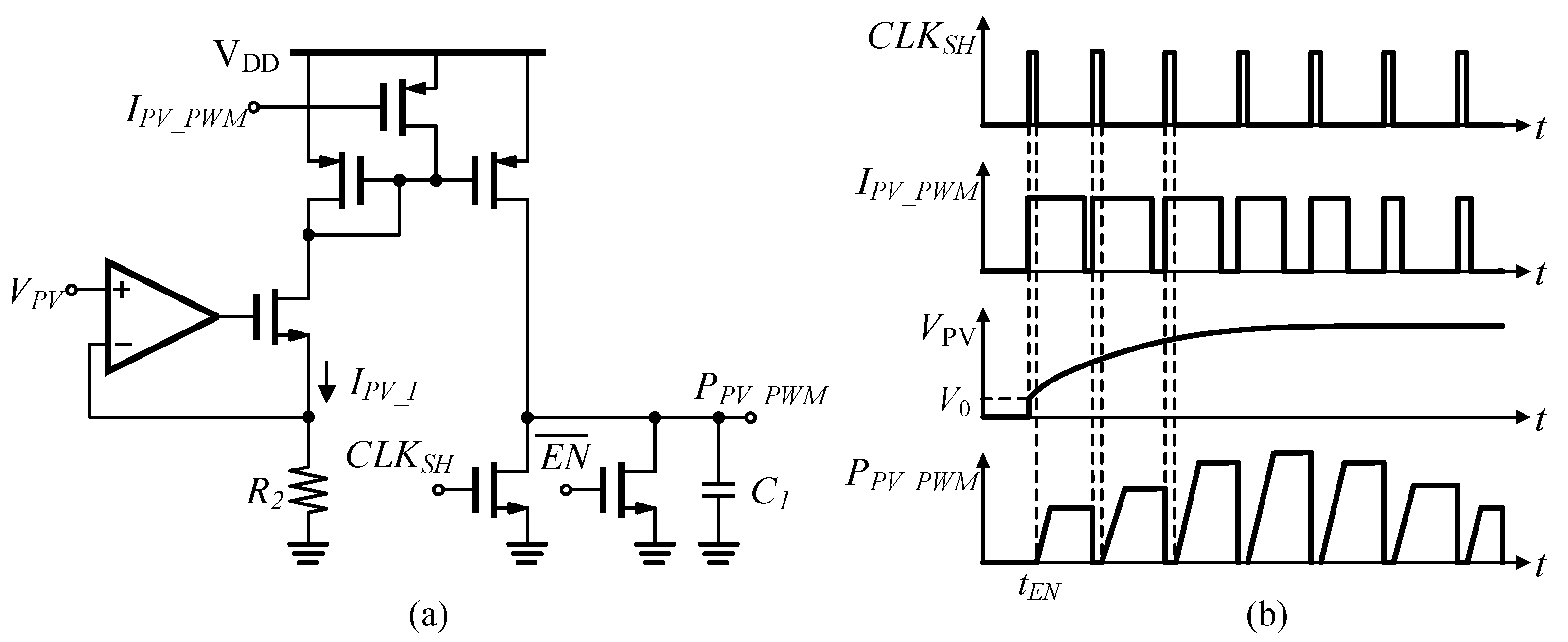
Figure 10 shows the block diagram and the timing diagram of the multiplier. The proposed multiplier calculates the power of the PV cell. For consuming low power, the proposed multiplier is implemented with analog circuits. The voltage form of the power of the PV cell, is calculated by the amount of energy in capacitor . The current form of ( can be expressed as
where is the value of a resistor. charges the capacitor, , during that is high. Calculated, the power of the PV cell, , can be expressed as Equation (5).
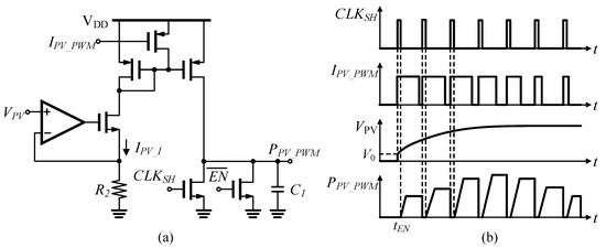
Figure 10.
(a) The block diagram and (b) the timing diagram of the multiplier.
Using Equations (4)–(6) can be expressed as
Using the Equations (2) and (7) can be expressed as
3.2. Set Phase
3.2.1. Sample and Hold (S & H)
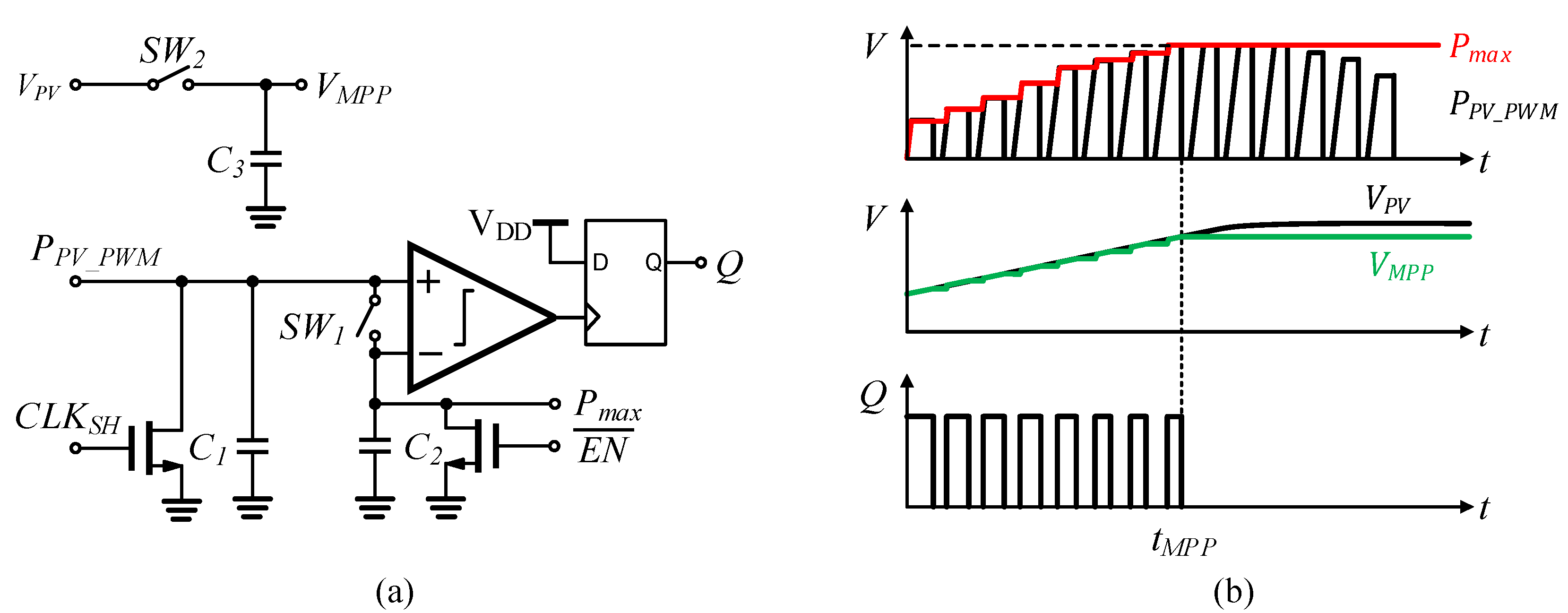
Figure 11 shows the block diagram and the timing diagram of the proposed sample and hold (S & H) circuit. In the S & H circuit, the MPP is tracked by comparing the current power, , that is stored in , with the previous maximum power, , that is stored in . If is lower than , the output of D flip-flop is low, then move to next iteration. If is higher than , is high, thus is on. Then, stores the new value of maximum power, , via charge sharing. can be expressed as
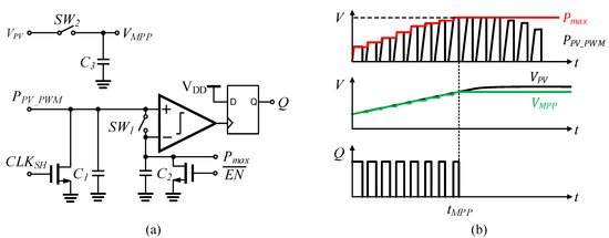
Figure 11.
(a) The block diagram and (b) the timing diagram of the sample and hold (S & H).
If is much higher than , Equation (9) can be expressed as
At the same time, is also on and the previous value of the , , is replaced by . After all iterations are done, the point that has the final value of and is the maximum power point. We can track the MPP timing by all these iterations.
3.2.2. Proposed FOCV
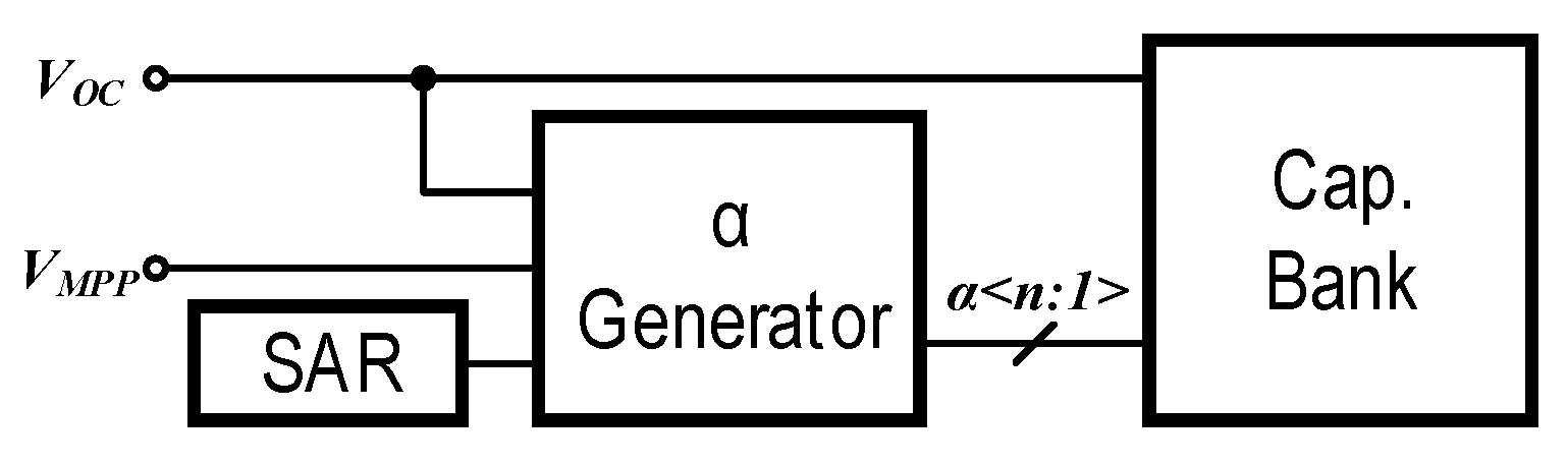
Figure 12 shows a simplified block diagram of the proposed FOCV that is composed of an generator, which is an analog-digital converter based on the SAR algorithm, and a capacitor bank. With two inputs of and , the generator generates a digital n-bit signal, , that represents the ratio of to based on the successive approximate register (SAR) algorithm. The relationship between these two signals can be expressed as
where is an n-bit digital signal.
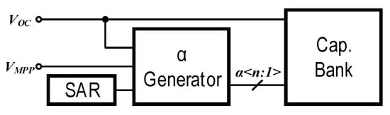
Figure 12.
The block diagram of the proposed FOCV circuit.
Figure 13 shows the detailed block diagram of the capacitor bank circuit inside the proposed FOCV circuit as well as the internal capacitor array circuit. Variable capacitors and consist of a number of unit capacitor, . The relation between these capacitors can be expressed as
where n is a natural number.
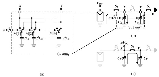
Figure 13.
The detailed block diagram of the cap bank circuit inside the proposed FOCV circuit; (a) the block diagram of the C-array circuit, (b) phase 1, and (c) phase 2.
The proposed FOCV circuit operates with two phases. In the first phase, switch S1 and switch S3 are closed, and switch S2 is open. Then, charges in . The energy charged in can be expressed as Equation (12).
In the second phase, the S1 and the S3 are open, and the S2 is closed, generating via charge sharing of . The energy charged in the and the can be expressed as Equation (13).
4. Simulation Results
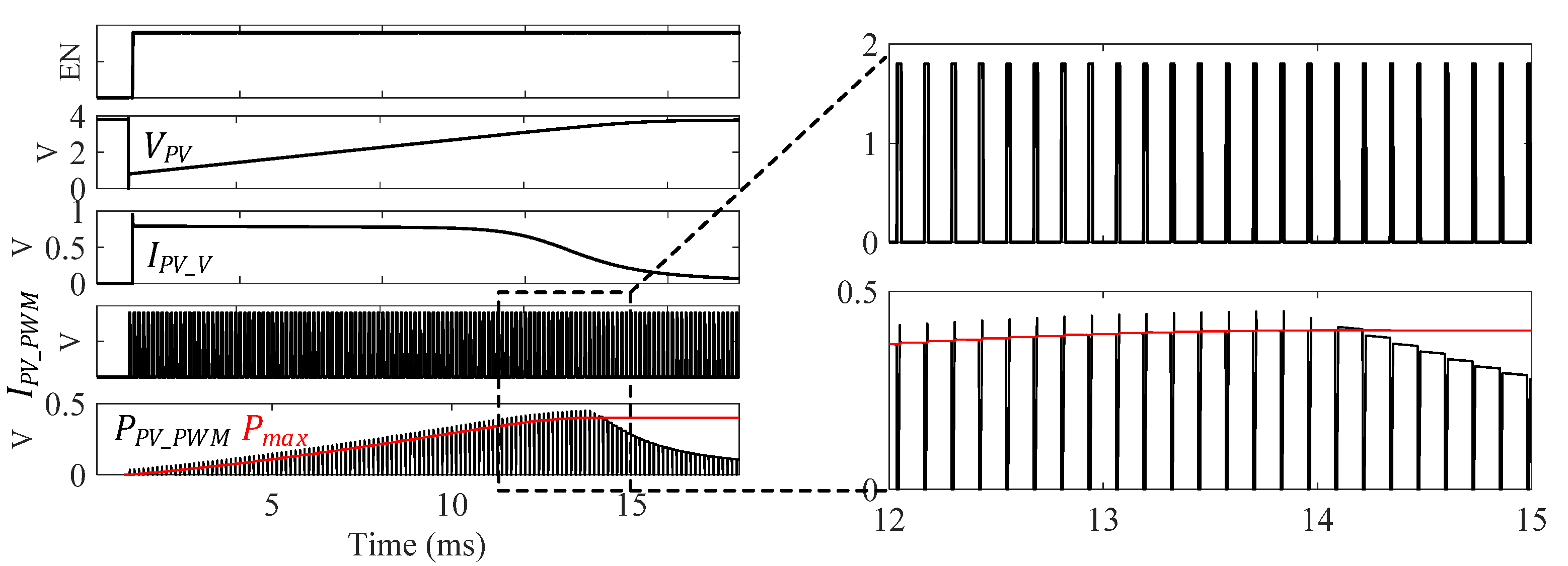
To validate the potentiality of the proposed FOCV MPPT algorithm, the proposed system is simulated with an electrically modeled PV cell that has the value of and , 3.79 V and 100 μA, respectively. Furthermore, is set in 8-bit resolution in the proposed FOCV circuit for the 99.6% tracking efficiency of The Cadence Spectre with TSMC 0.18 μm process parameters was used for SPICE (Integrated Circuit Emphasis) simulation. Figure 14 shows the simulation results of the operating voltage, , , , and , and the maximum power point tracking in the time domain of the proposed FOCV MPPT algorithm.

Figure 14.
Simulation results of the maximum power point tracking for the proposed FOCV MPPT.
Figure 15 shows the simulation result of the comparison of the energy loss between the conventional and the proposed FOCV MPPT under varying . The total simulated period was 4 h and the refreshing period of the proposed FOCV MPPT was 30 min; the varies every 1 h. The energy loss of the conventional and the proposed FOCV were 356.37 mWs and 0.09 mWs, respectively. The energy loss of the proposed FOCV decreased by 99.97% compared to that of the conventional FOCV. The simulated result shows that the proposed FOCV can reduce the energy loss tremendously compared to the conventional FOCV.
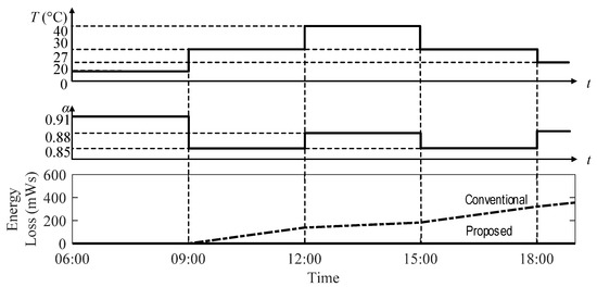
Figure 15.
Simulated results of the energy loss for the conventional FOCV and the proposed FOCV MPPT under varying .
5. Experimental Results
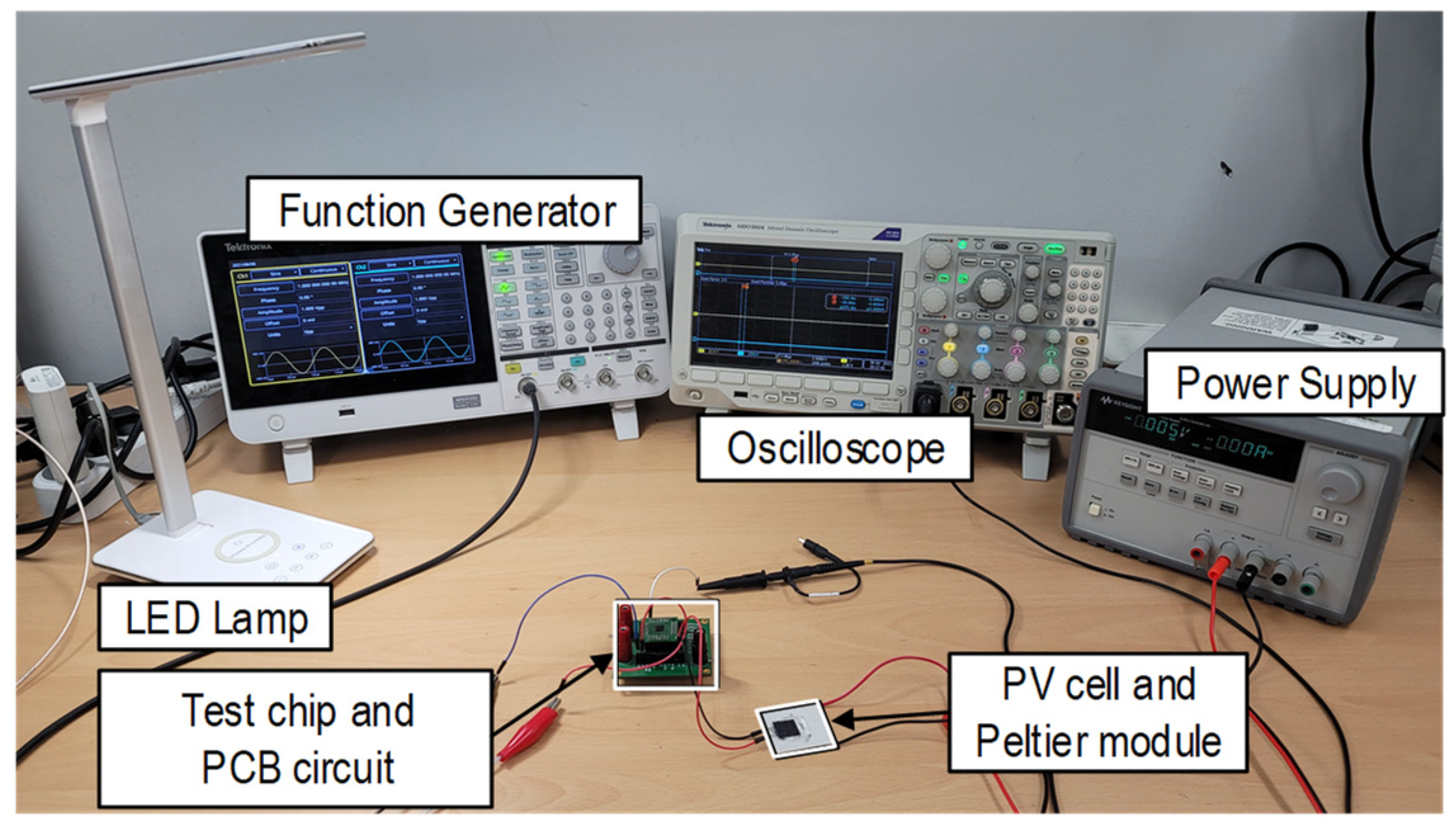
The proposed FOCV MPPT circuit was in a 0.18-μm CMOS process. Figure 16 shows a microphotograph of the fabricated chip. The proposed FOCV MPPT circuit occupies an area of 750 × 300 μm2. Figure 17 shows the experimental setup. A 5-W LED lamp (Power Stand-X1) and the neutral density filter (Kenko ND) was used for the varying illuminance condition instead of solar irradiance. A PV cell was attached on the Peltier module for the varying temperature condition. The specifications of the PV cell (AM-1815) were , , and under the condition of 200 lx and 25 °C. Under the experimental conditions, the specifications were , , and , respectively.
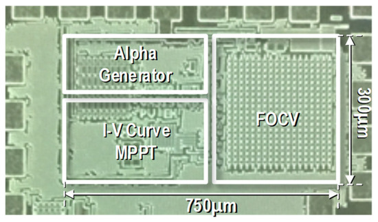
Figure 16.
Chip micrograph.
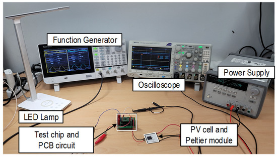
Figure 17.
Experimental setup for the proposed FOCV MPPT.
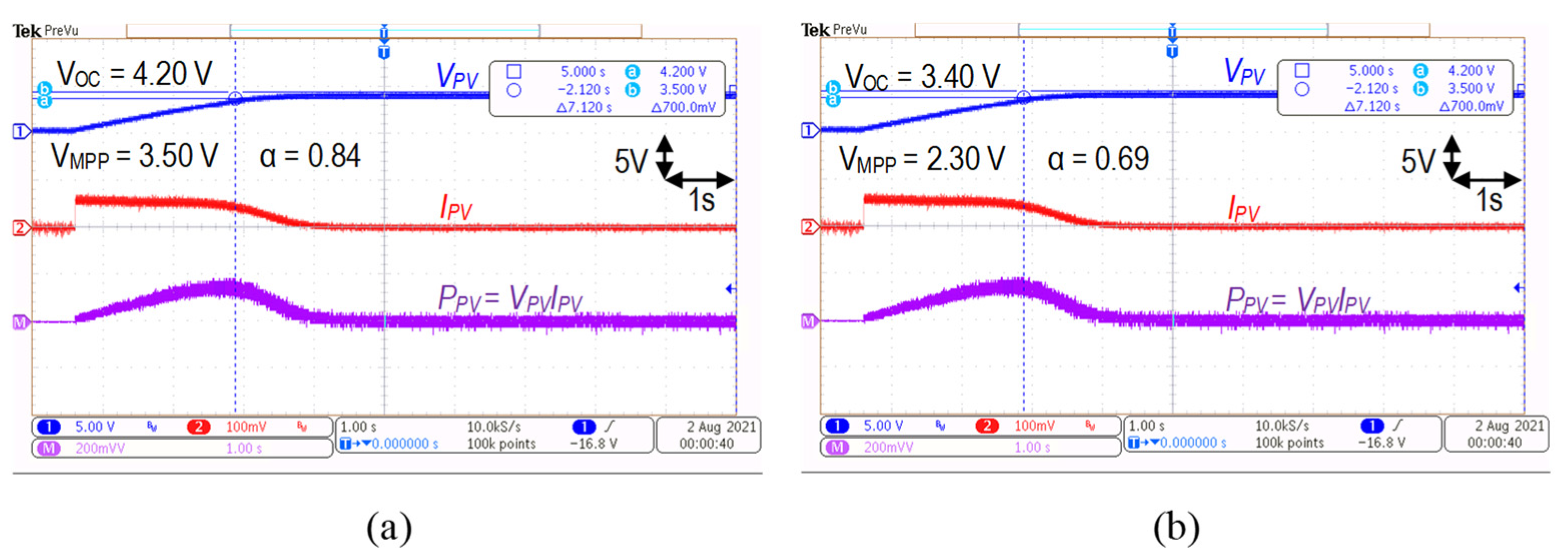
Figure 18 shows the measured I-V curves and the valuesat 25 °C and 65 °C. As the temperature varied from 25 °C to 65 °C, not only did and change, from 4.20 V to 3.40 V and from 3.50 V to 2.30 V, respectively, but also changes significantly from 0.84 to 0.69, a 17.86% difference.

Figure 18.
Measured I-V curves and of PV cell under various temperature: (a) 25 °C, (b) 65 °C.
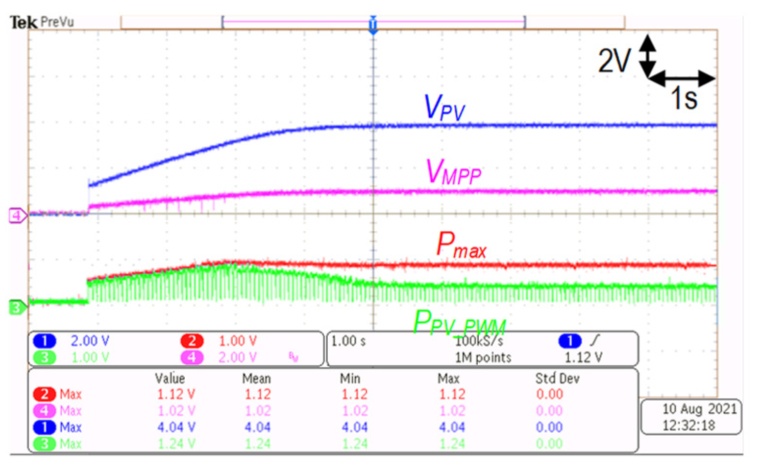
The measured MPP tracking waveforms and the operating voltages (, , , and ) are shown in Figure 19. In Figure 19, the operating points of the PV cell track the MPP according to the proposed FOCV MPPT algorithm.
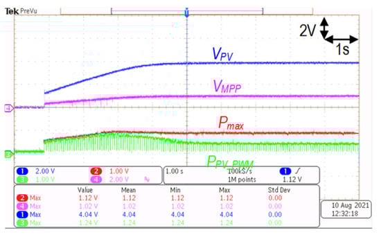
Figure 19.
Measured power tracking waveforms with the proposed FOCV MPPT under 25 °C.
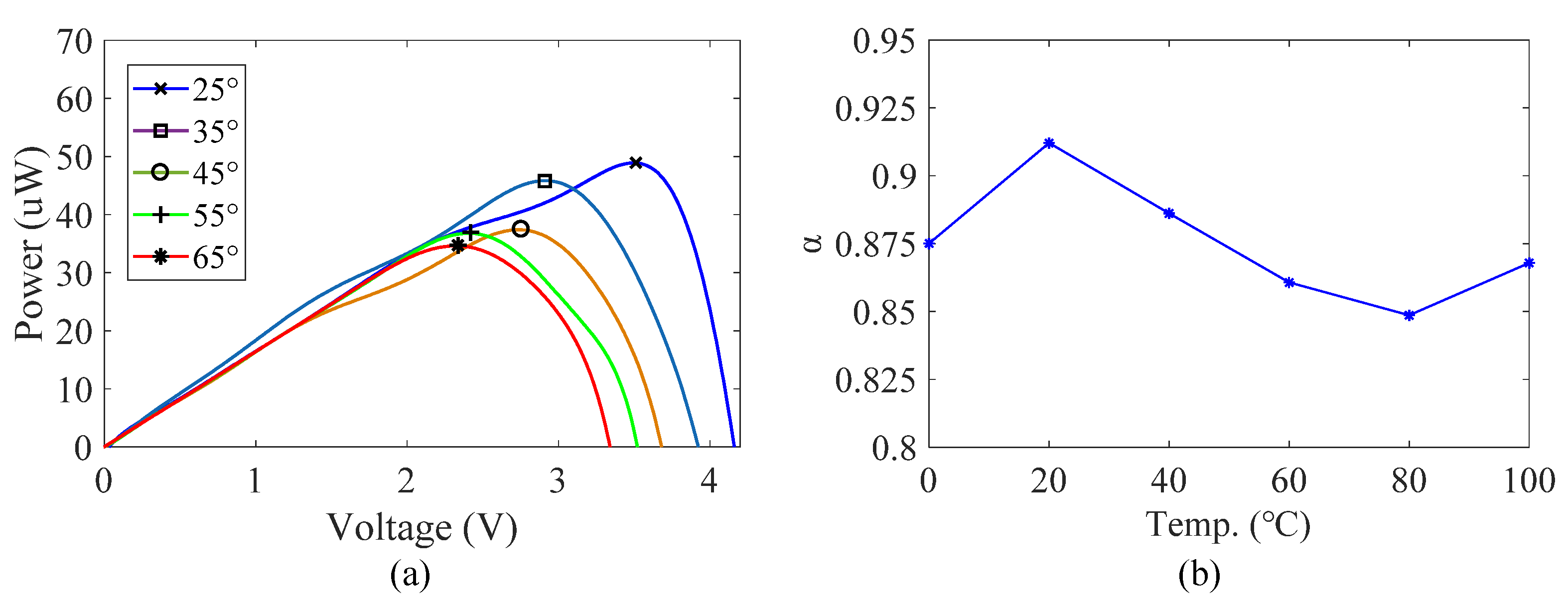
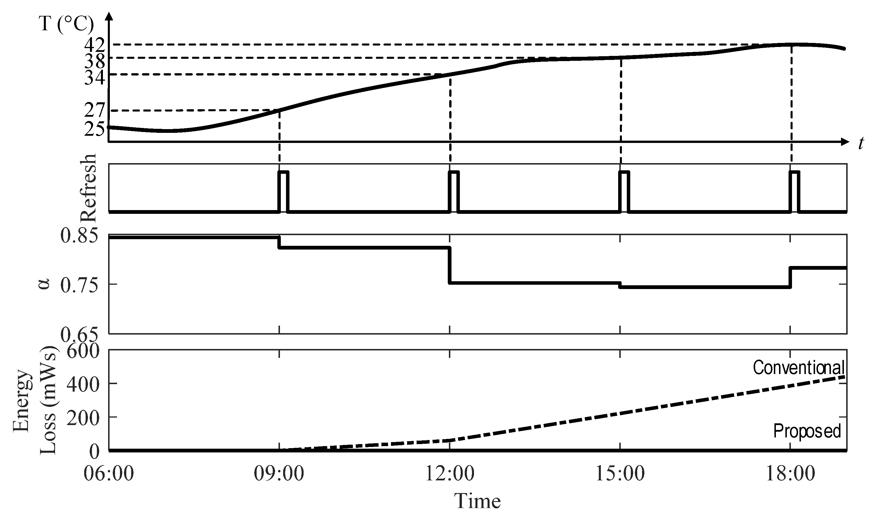
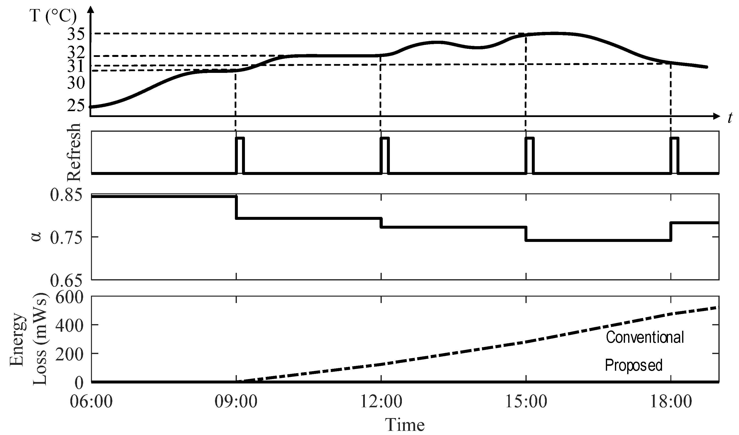
Figure 20 shows the measured varying P-V characteristics and of the PV cell under various temperature conditions, from 25 °C to 65 °C. Even in the single PV cell, varied significantly depending on temperature variation from 0.85 to 0.69. Comparison of the energy loss caused by wrong between the conventional FOCV and the proposed FOCV MPPT with the refreshing frequency for 13 h under varying temperature conditions is shown in Figure 21 and Figure 22. Each temperature daily profile was measured at Death Valley, California, USA on 30 April, 2021 [34] (Scenario I), and Seoul, South Korea on 30 July 2021 [35] (Scenario II), respectively. According to Figure 21, the energy loss of the conventional FOCV and the proposed FOCV MPPT were 441.12 mWs and 0.25 mWs, respectively while the temperature varied from 25 °C at 06:00 to 42 °C at 18:00. The energy loss by the proposed FOCV decreased by 99.94% of that of the conventional FOCV per hour. In Figure 22, the energy loss of the conventional and the proposed FOCV are 521.71 mWs and 0.36 mWs, respectively; the proposed FOCV reduced the energy loss by 99.93% compared the conventional FOCV.
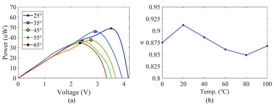
Figure 20.
Experimental results for (a) power versus voltage characteristics a PV cell and (b) under various temperatures: 25, 35, 45, 55, and 65 °C.

Figure 21.
Calculated energy loss based on experimental results in Figure 20 for the conventional and the proposed FOCV MPPTs with the daily temperature profile at Death Valley on 30 April 2021 (Scenario I).

Figure 22.
Calculated energy loss based on experimental results in Figure 20 for the conventional and the proposed FOCV MPPTs with the daily temperature profile at Seoul, South Korea on 30 July 2021 (Scenario II).
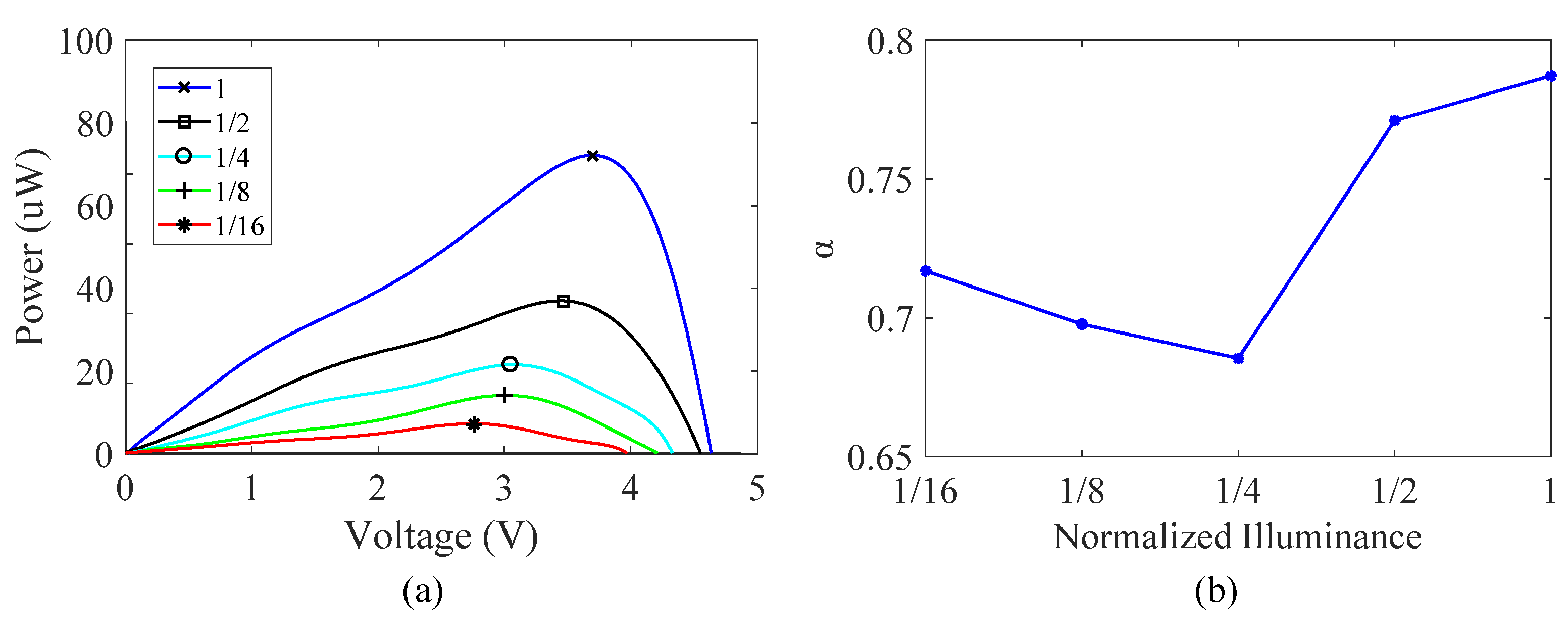
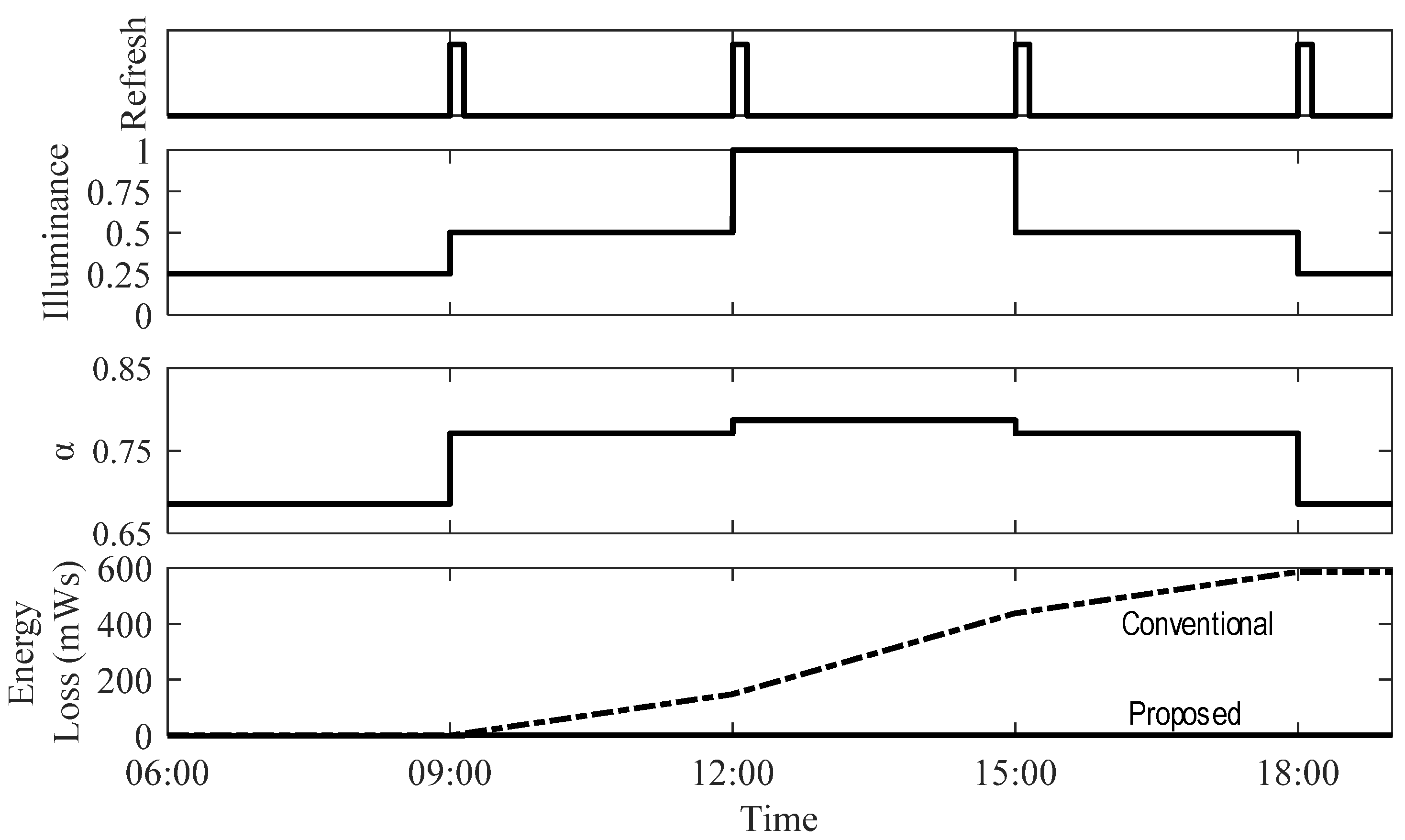
Figure 23 shows the measured varying P-V characteristics and of the PV cell under varying illuminance conditions, from the normalized illuminance 1 to 1/16. Each illuminance step is quantized by the distance and the neutral-density filter and normalized by the Illuminance-1 that was measured under a 0.3-m distance between the PV cell and the LED lamp. As shown in Figure 23b, varies significantly from 0.69 to 0.79 depending on illuminance. Figure 24 illustrates comparison of the energy loss between the conventional and the proposed FOCV with the refreshing frequency, , under varying illuminance over 13 h (Scenario III). In Figure 24, the energy loss caused by the conventional and the proposed FOCV are 585.58 mWs and 0.35 mWs, respectively. According to Figure 23, the energy loss by the proposed FOCV decreased by 99.94% of that of the conventional FOCV.
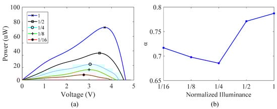
Figure 23.
Measured (a) power versus voltage characteristics and (b) of a PV cell under various normalized illuminance.
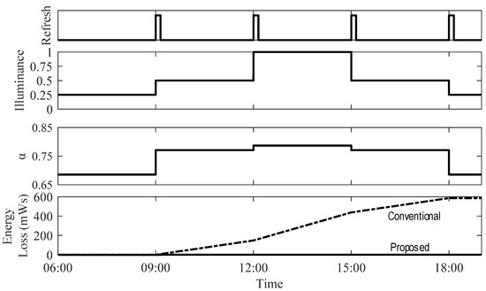
Figure 24.
Calculated energy loss for the conventional and the proposed FOCV MPPTs under varying normalized illuminance (Scenario III).
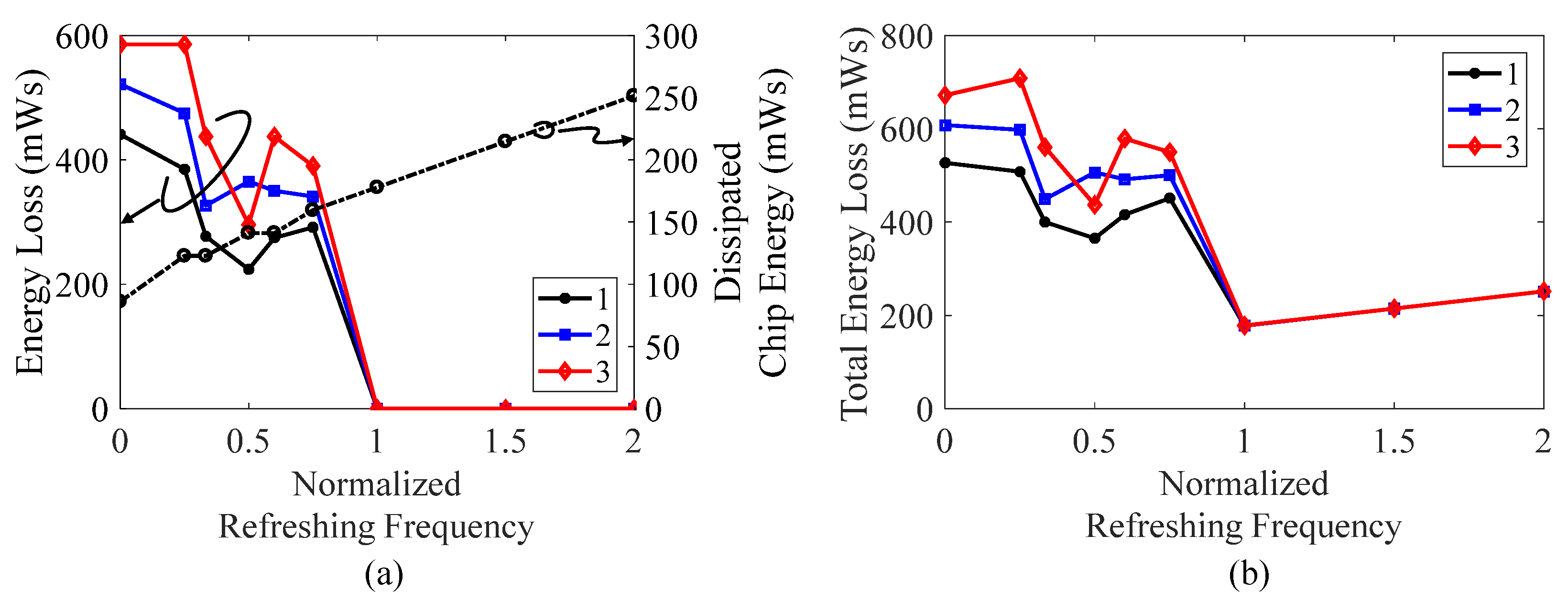
Figure 25 compares energy losses of a PV cell and the proposed FOCV MPPT according to refreshing frequency under three scenarios. In Figure 25a, the energy loss in a PV cell depends on the refreshing frequency of , where refreshing frequencies are normalized by . The energy dissipation of the proposed control is proportional to the refreshing frequency. The energy loss reaches to almost zero when the refreshing frequency is higher than or equal to one. The total energy loss of the system, including a PV cell and the MPPT control, is the sum of the energy loss and the dissipated chip energy. Figure 25b indicates that the total energy loss of the proposed system can be minimized when the refreshing frequency is one.
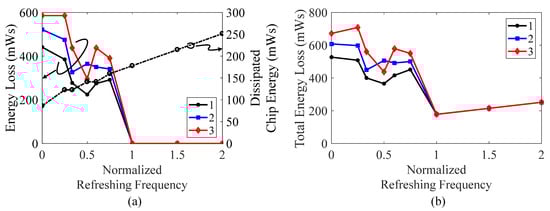
Figure 25.
Proposed FOCV MPPT according to refreshing frequency under three scenarios. (a) energy loss and the dissipated chip energy, (b) total energy loss (the sum of energy loss and dissipated chip energy).
6. Conclusions
In this paper, an intermittent FOCV MPPT using an I-V curve tracer is proposed as a solution for energy loss caused by the mismatch of due to varying environmental conditions like temperature and illuminance. To minimize energy loss, the proposed FOCV MPPT system is designed to dynamically scan the I-V curve of a PV cell to detect the GMPP, not the local MPP, and intermittently reset the MPP for varying environmental conditions. The proposed FOCV MPPT system sets in 8-bit resolution. As the chip power consumption is relatively small compared to the PV cell rated power, the proposed FOCV MPPT system with a refreshing frequency higher than the environmental change substantially reduces the energy loss, by up to 99.9% as compared to a conventional FOCV, based on daily environmental conditions.
Author Contributions
Conceptualization, Y.C.I. and Y.S.K.; methodology, Y.C.I.; validation, Y.C.I., J.P. and Y.S.K.; formal analysis, Y.C.I.; investigation, Y.C.I. and J.P.; data curation, Y.S.K.; writing—original draft preparation, Y.C.I. and Y.S.K.; writing—review and editing, Y.C.I. and Y.S.K.; visualization, Y.C.I., S.S.K. and J.P.; supervision, Y.S.K.; project administration, Y.S.K. All authors have read and agreed to the published version of the manuscript.
Funding
This research received no external funding.
Institutional Review Board Statement
Not applicable.
Informed Consent Statement
Not applicable.
Data Availability Statement
Data sharing is not applicable to this article.
Acknowledgments
This work was supported in part by the Basic Science Research Program through the National Research Foundation of Korea (NRF), Ministry of Education, under Grant NRF-2021R1A2C2014652. This work and the chip fabrication were supported by the IC Design Education Center (IDEC).
Conflicts of Interest
The authors declare no conflict of interest.
References
- Lin, K.; Yu, J.; Hsu, J.; Zahedi, S.; Lee, D.; Friedman, J.; Kansal, A.; Raghunathan, V.; Srivastava, M. Heliomote: Enabling Long-lived Sensor Networks through Solar Energy Harvesting. In Proceedings of the 3rd International Conference on Embedded Networked Sensor Systems, San Diego, CA, USA, 2–4 November 2005. [Google Scholar]
- Beeby, S.P.; Tudor, M.J.; White, N.M. Energy Harvesting Vibration Sources for Microsystems Applications. Meas. Sci. Technol. 2006, 17, 175–195. [Google Scholar] [CrossRef]
- Wu, L.; Ha, D.S. A Self-Powered Piezoelectric Energy Harvesting Circuit with an Optimal Flipping Time SSHI and Maximum Power Point Tracking. IEEE Trans. Circuits Syst. II Express Briefs 2019, 10, 1758–1762. [Google Scholar] [CrossRef]
- Lawrence, E.E.; Snyder, G.J. A Study of Heat Sink Performance in Air and Soil for Use in a Thermoelectric Energy Harvesting Device. In Proceedings of the Twenty-First International Conference on Thermoelectrics, Long Beach, CA, USA, 29 August 2002. [Google Scholar]
- Sher, H.A.; Murtaza, A.F.; Noman, A.; Addoweesh, K.E.; Al-Haddad, K.; Chiaberge, M. A New Sensorless Hybrid MPPT Algorithm Based on Fractional Short-Circuit Current Measurement and P&O MPPT. IEEE Trans. Sustain. Energy 2015, 6, 1426–1434. [Google Scholar]
- Kim, H.; Kim, S.; Kwon, C.; Min, Y.; Kim, C.; Kim, S. An Energy-Efficient Fast Maximum Power Point Tracking Circuit in an 800-uW Photovoltaic Energy Harvester. IEEE Trans. Power Electron. 2013, 28, 2927–2935. [Google Scholar] [CrossRef]
- Liu, S.; Dougal, R.A. Dynamic Multiphysics Model for Solar Array. IEEE Trans. Energy Convers. 2002, 17, 285–294. [Google Scholar]
- Hong, Y.; Pham, S.N.; Yoo, T.; Chae, K.; Baek, K.; Kim, Y.S. Efficient Maximum Power Point Tracking for a Distributed PV System under Rapidly Changing Environmental Conditions. IEEE Trans. Power Electron. 2015, 30, 4209–4218. [Google Scholar] [CrossRef]
- Esram, T.; Chapman, P.L. Comparison of Photovoltaic Array Maximum Power Point Tracking Techniques. IEEE Trans. Energy Convers. 2007, 22, 439–449. [Google Scholar] [CrossRef] [Green Version]
- Masoum, M.A.S.; Dehbonei, H.; Fuchs, E.F. Theoretical and Experimental Analyses of Photovoltaic Systems with Voltage- and Current-Based Maximum Power-Point Tracking. IEEE Trans. Energy Convers. 2002, 17, 514–522. [Google Scholar] [CrossRef] [Green Version]
- Brunelli, D.; Moser, C.; Thiele, L.; Benini, L. Design of a Solar-Harvesting Circuit for Batteryless Embedded Systems. IEEE Trans. Circuits Syst. I Regul. Pap. 2009, 11, 2519–2528. [Google Scholar] [CrossRef]
- Wang, Y.; Liu, Y.; Wang, C.; Lil, Z.; Sheng, X.; Lee, H.G.; Chang, N.; Yang, H. Storage-Less and Converter-Less Photovoltaic Energy Harvesting with Maximum Power Point Tracking for Internet of Things. IEEE Trans. Comput.-Aided Des. Integr. Circuits Syst. 2016, 35, 173–186. [Google Scholar] [CrossRef]
- Wang, J.; Li, J.; Ha, D.S. Energy Harvesting Circuit for Indoor Light based on the FOCV and P&O Schemes with an Adaptive Fraction Approach. In Proceedings of the 2020 IEEE International Symposium on Circuits and Systems (ISCAS), Seville, Spain, 10–21 October 2020. [Google Scholar]
- Femia, N.; Petrone, G.; Spagnuolo, G.; Vitelli, M. Optimization of Perturb and Observe Maximum Power Point Tracking Method. IEEE Trans. Power Electron. 2005, 20, 963–973. [Google Scholar] [CrossRef]
- Krishlnan, M.M.; Bharath, K.R. A Novel Sensorless Hybrid MPPT Method Based on FOCV Measurement and P&O MPPT Technique for Solar PV Applications. In Proceedings of the 2019 International Conference on Advances in Computing and Communication Engineering (ICACCE), Sathyamangalam, India, 4–6 April 2019. [Google Scholar]
- Canadian_Solar-Datasheet- BiHiKu_CS3W-PB-AG_High Efficiency_(1000 V & 1500 V). Available online: https://www.canadiansolar.com/wp-content/uploads/2019/12/Canadian_Solar-Datasheet-BiHiKu_CS3W-PB-AG_High-Efficiency_1000V1500V_EN-2.pdf (accessed on 27 June 2021).
- JKM395-415M-54HL4-V-F1-30-CN.ai. Available online: https://www.jinkosolar.com/uploads/JKM395-415M-54HL4-V-F1-30-CN.pdf (accessed on 27 June 2021).
- JKM440-460M-60HL4-(V)-F1-CN.ai. Available online: https://www.jinkosolar.com/uploads/JKM440-460M-60HL4-(V)-F1-CN.pdf (accessed on 27 June 2021).
- PS-M A Datasheet_TALLMAX_DE06X.05(II)_EN_2020_PA2_web. Available online: https://static.trinasolar.com/sites/default/files/US_Datasheet_DE06X.05(II)_NA_2021_PA3.pdf (accessed on 27 June 2021).
- Download | Panasonic Solar HIT | Life Solutions | Business | Panasonic Global. Available online: http://panasonic.net/lifesolutions/solar/download/index.html (accessed on 27 June 2021).
- VBHN330_325SJ47_EN.pdf. Available online: http://europe-solarstore.com/download/panasonic/VBHN330_325SJ47_EN.pdf (accessed on 20 August 2021).
- PS-M- Small Size Datasheet_TallmaxM_DEG15VC.20(II)_EN_2020_PA1_web. Available online: http://static.trinasolar.com/sites/default/files/Datasheet_Bifacial%20DEG15VC.20%28II%29_2021_B.pdf (accessed on 27 June 2021).
- Datasheets. Available online: http://q-cells.com/kr/main/service/download/datasheets~datasheets~.html?page=1 (accessed on 27 June 2021).
- Canadian_solar-Datasheet- HiKu_CS3N-MS_(1000 V & 1500 V)_EN. Available online: https://static.csisolar.com/wp-content/uploads/sites/2/2019/12/13140918/CS-Datasheet-HiKu_CS3N-MS_v2.8C25_AU-black-frame25-years-product-warranty.pdf (accessed on 27 June 2021).
- JAM72S10 400-420 MR. Available online: https://www.jasolar.com//uploadfile/2020/0605/20200605034219227.pdf (accessed on 27 June 2021).
- JAM60S10 330-350 MR. Available online: https://www.jasolar.com//uploadfile/2020/0605/20200605033853385.pdf (accessed on 27 June 2021).
- LR5-66HBD 475-500M. Available online: http://en.longi-solar.com/uploads/attach/20210507/60950dbad3c23.pdf (accessed on 27 June 2021).
- LGiLE-T-TMD-059-108 LR5-72HBD 525-545M. Available online: http://en.longi-solar.com/uploads/attach/20210512/609b53096a2a1.pdf (accessed on 27 June 2021).
- EN_Ultra_S_STP455S_B72_Vnh.pdf. Available online: http://suntech-power.com/wp-content/uploads/download/product-specification/EN_Ultra_S_STP455S_B72_Vnh.pdf (accessed on 27 June 2021).
- EN_Ultra_V_STP550S_C72_Vmh.pdf. Available online: http://suntech-power.com/wp-content/uploads/download/product-specification/EN_Ultra_V_STP550S_C72_Vmh.pdf (accessed on 27 June 2021).
- 83e8173f1203f01571b4170ae1827bbe.pdf. Available online: http://www.tw-solar.com/en/Uploads/20210409/83e8173f1203f01571b4170ae1827bbe.pdf (accessed on 27 June 2021).
- 2230b50c83aaf4092bd129beb1352d3d.pdf. Available online: http://www.tw-solar.com/en/Uploads/20210409/2230b50c83aaf4092bd129beb1352d3d.pdf (accessed on 27 June 2021).
- 2e414aeb51a11620dc-45d1a08f722a1e.pdf. Available online: http://www.tw-solar.com/en/Uploads/20210409/2e414aeb51a11620dc45d1a08f722a1e.pdf (accessed on 27 June 2021).
- Weather in April 2021 in Furnace Creek (Death Valley), California, USA. Available online: http://timeanddate.com/weather/usa/furnace-creek-death-valley/historic?month=4&year=2021 (accessed on 16 August 2021).
- Weather in July 2021 in Seoul, South Korea. Available online: http://timeanddate.com/weather/south-korea/seoul/historic?month=7&year=2021 (accessed on 17 August 2021).


Publisher’s Note: MDPI stays neutral with regard to jurisdictional claims in published maps and institutional affiliations. |
© 2021 by the authors. Licensee MDPI, Basel, Switzerland. This article is an open access article distributed under the terms and conditions of the Creative Commons Attribution (CC BY) license (https://creativecommons.org/licenses/by/4.0/).