Abstract
Engineers widely use topology optimization during the initial process of product development to obtain a first possible geometry design. The state-of-the-art method is iterative calculation, which requires both time and computational power. This paper proposes an AI-assisted design method for topology optimization, which does not require any optimized data. An artificial neural network—the predictor—provides the designs on the basis of boundary conditions and degree of filling as input data. In the training phase, the so-called evaluators evaluate the generated geometries on the basis of random input data with respect to given criteria. The results of those evaluations flow into an objective function, which is minimized by adapting the predictor’s parameters. After training, the presented AI-assisted design procedure generates geometries that are similar to those of conventional topology optimizers, but require only a fraction of the computational effort. We believe that our work could be a clue for AI-based methods that require data that are difficult to compute or unavailable.
1. Introduction
The presented paper deals with the solution of optimization problems by means of artificial intelligence (AI) techniques. Topology optimization (TO) was chosen as an application example, even though the described method is applicable to many optimization problems and thus has generality.
TO is a method of calculating a shape (topology). In TO, the material distribution over a given design domain is the subject of optimization by minimizing a given objective function while satisfying given constraints [1]. In most cases, suitable search algorithms solve the optimization problem mathematically.
The combination of AI and TO in the state-of-the-art research mostly requires optimized geometries or intermediate results generated by conventional TO. For this reason, they are subject to several limitations that affect those techniques, such as large computational effort and the need to prepare representative data.
The approach proposed here aims at removing those drawbacks by generating all the artificial knowledge required for optimization during the learning phase, with no need to rely on pre-optimized results.
1.1. Topology Optimization
In this work, only the case of mono-material topology optimization is considered. The material of which the structure is to be build is a constant of the problem, and the geometry remains unknown.
The function to be minimized in stiffness optimization is usually the scalar measure of structural compliance. In addition, the material quantity condition must be fulfilled. This material quantity corresponds to the fraction of the maximum possible amount of material (degree of filling) and is often also referred to as the volume fraction. The minimization of compliance results in maximizing the stiffness [2,3]. Typically considered restrictions are the available design domain, the static and kinematic boundary conditions for the regarded load cases as well as strength thresholds.
There are numerous possible approaches to TO [1]. According to the “Solid Isotropic Material with Penalization” (SIMP) approach of Bendsøe [2], a subdivision of the design domain into elements takes place. A factor, yet to be determined, scales the contribution of each element to the overall stiffness of the structure.
The SIMP approach is able to provide optimized geometries for many practical cases by means of an iterative process. Each iteration involves computationally intensive operations: the most critical ones are assembling the stiffness matrix and solving the system’s equation. The involvement of restrictions, such as stress restrictions, increases the complexity of the optimization problem [4,5].
1.2. Artificial Neural Networks
Artificial neural networks (ANNs) belong to the area of machine learning (ML), which, in turn, are assigned to AI. ANNs are able to learn and execute complex procedures, which has led to remarkable results in recent years. ANNs or, more precisely, feedforward neural networks, consist of layers connected in sequence. These layers contain so-called neurons [6]. A neuron (see Figure 1) is the basic element of an ANN. The combination of all layers is also called a network.

Figure 1.
Graphical representation of the calculation procedure of a single neuron.
The neuron receives n inputs (here given as vector ), which are linearly combined and added to a bias value b and passed as argument to an activation function as follows:
The coefficients of the linear combination, collected in the vector , are called weights.
It is usual that several neurons have the same input. All neurons with the same inputs are grouped together in one layer (also called the fully connected layer). Since one single output is supplied by each neuron, each layer with m neurons also produces m outputs, and the weights become matrices . The outputs of a layer (except the last layer) serve as inputs for the following layer. The first layer is called input layer and the last layer is called output layer . Any layer whose input and output values are not accessible to the user is called hidden layer . Each layer, for example, layer , has its own weights and biases .
The number of layers nL is also named the depth of the network, which also originate the attribute “deep” in the term deep learning (DL). The term DL is generally used for ANNs with several hidden layers. The presence of several layers makes it possible to map a more complex transfer behavior between the input and the output layer.
The functional relationship
realized by the ANN depends on the weights and on the biases , which are adjusted in the context of so-called training or learning, according to certain algorithms (learning algorithms). The learning algorithm used consists of the gradient-based minimization of a scalar value termed error or loss, which is obtained from the deviations of the actual outputs from given target outputs. The values, which describe the network’s architecture and do not undergo any change during training, such as the number of neurons in a layer, are termed hyperparameters.
In addition to the fully connected layers, there are convolutional layers. These layers use convolution in place of the linear combination (1). Here, the trainable weights, also called the convolution kernel, are convoluted with the input of the layer and produce an output, which is passed to the next layer. This process is efficient for grid-like data structures and is, therefore, used for many modern image applications [7,8].
The output of an ANN is henceforth referred to as prediction. Further details on the learning of an ANN can be found in the specific literature, for example, [7,9].
1.3. Deep Learning–Based Topology Optimization
DL-based TO, by predicting the geometry through ANNs, aims to deliver optimized results in only a fraction of the time required by conventional optimization, by moving the computationally intensive part to the training algorithm, which executes only once. The trained ANN provides results which can be used directly, refined with conventional methods or adapted to the desired structure size.
There have already been some attempts in this area. Some approaches [10,11,12,13,14,15,16] used an ANN or a generative adversarial network (GAN) [17] to map the boundary conditions directly to the desired optimized geometries. They, therefore, required many thousands of topology-optimized geometries as training data points for the ANN and achieved near-optimal results in terms of geometric similarity. Zhang et al. and Nie et al. used some physical fields over the initial domain, such as strain energy density or von Mises stress, for the training of the neural network [18,19]. Banga et al. used an approach in which intermediate results of conventional TO are the basis for the training data points for the ANN, which is able to produce 3D geometries [20]. Yamasaki et al. used a data-driven approach, which is characterized by selecting the best data points for training [21]. Cang et al. used a theory-driven approach in which two cases were trained and tested. In the first case, the direction of a single load could be changed. The second case had variable directions as well as the positions of the load [22]. A different approach was presented by Chandrasekhar and Suresh, where the ANN does not generate the whole geometry but only a density value at given x and y coordinates. This method provides very good results at high resolution and is also applicable to the 3D case. A disadvantage is that the training must be repeated when the boundary conditions are modified [23].
Sosnovik and Oseledets used DL to speed up conventional TO by [24] by using the results from some conventional TO iterations as input for the ANN. Qian and Ye accelerated conventional TO by utilizing surrogate models for forward and sensitivity calculations [25]. These approaches are indirect since some iterations are required.
Although such DL-based TO procedures are able to perform the above-mentioned task of a fast and mostly direct generation of optimized geometries, the predictions undergo some restrictions.
State-of-the-art procedures require the use of large number of optimized training data points. These training data points must be optimal to be suitable as training data. Depending on the optimization formulation, this may be not the case, as local minima and convergence problems may occur. A method that does not use optimized data is not subject to these restrictions.
Since topology-optimized training data are used, and the generation of these data with conventional methods is very time consuming, the number of training data points that can be considered is limited. In the case of [10], 100,000 training data points were generated; this took about 200 h. Another 8 h were needed for training. This limitation affects the accuracy in the prediction of unknown geometries (i.e., geometries which were not used within the training) negatively.
For those approaches that do not require optimized data, but require initial or intermediate results of conventional TO, the input data points must be available prior to training. Therefore, the aforementioned limitation persists.
This paper investigates the possibility, which differs from the state-of-the-art methods, to train an ANN without the use of optimized or computationally prepared data. The generation of training data points and the training itself are merged in one single procedural step, also called online training. Unlike existing approaches, the ANN does not need to be re-trained if the boundary conditions are altered.
This makes it possible to process a much larger amount of training data points for the training in a much shorter time. Since the objective function value, which is also the loss (see Section 2.7), is calculated during the training, the ANN learns to avoid undesirable results.
2. Method
The presented method is based on an ANN architecture called predictor–evaluator network (PEN), which was developed by the authors for this purpose. The predictor is the trainable part of the PEN and its task is to generate—based on input data—optimized geometries.
As mentioned, unlike the state-of-the-art methods, no conventionally topology-optimized or computationally prepared data are used in the training. The geometries used for the training are created by the predictor itself on the basis of randomly generated input data and evaluated by the remaining components of the PEN, called evaluators.
The evaluators perform mathematical operations. Other than the predictor, the operations performed by the evaluators are pre-defined and do not change during the training. It would also be possible to use evaluators based on an ANN.
Each evaluator assesses the outputs of the predictor with respect to a certain criterion and returns a corresponding scalar value as a measure of the criterion’s fulfillment. This fulfillment is the loss or the error of this evaluator. A scalar function of the evaluator outputs (objective function J, see Section 2.7) combines the individual losses.
During the training, the objective function computed for a set of geometries (batch) is minimized by changing the predictor’s trainable parameters; see Section 2.2. In this way, the predictor learns how to produce optimized geometries.
The predictor, the individual evaluators, their tasks and their way of operation are explained in detail in the following sections.
2.1. Basic Definitions
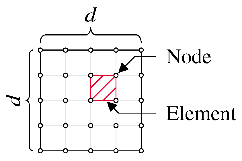
In topology optimization, the design domain is typically subdivided into elements by appropriate meshing. Figure 2 visualizes the elements (with one element hatched) and nodes.

Figure 2.
Design space overview with elements, nodes and dimension d (square case).
In this work, we examined only square meshes with equal numbers of rows and columns. However, this method can be used for non-square and three-dimensional geometries.
The total number of elements in the 2D case is as follows:
where is the number of rows and the number of columns (see Figure 2). In the square case, the number of rows and columns are equal: .
The design variables , termed density values, scale the contributions of the single elements to the stiffness matrix. The density has a value of one when the stiffness contribution of the element is fully preserved and zero when it disappears.
The density values are collected in a vector . In general, the density values are defined in the interval [0,1]. In order to prevent possible singularities of the stiffness matrix, a lower limit value for the entries of is set as follows [2]:
The vector of design variables can be transformed to a square matrix of order d by using the operator:
Although a binary selection of the density is desired (discrete TO, material present/not present), values between zero and one are permitted for algorithmic reasons (continuous TO). To get closer to the desired binary selection of densities, the so-called penalization can be used in the calculation of the compliance. The penalization is realized by an element-wise exponentiation of the densities by the penalization exponent [26].
The arithmetic mean of all defines the degree of filling of the geometry as follows:
The target value is the degree of filling that is to be achieved by the predictor.
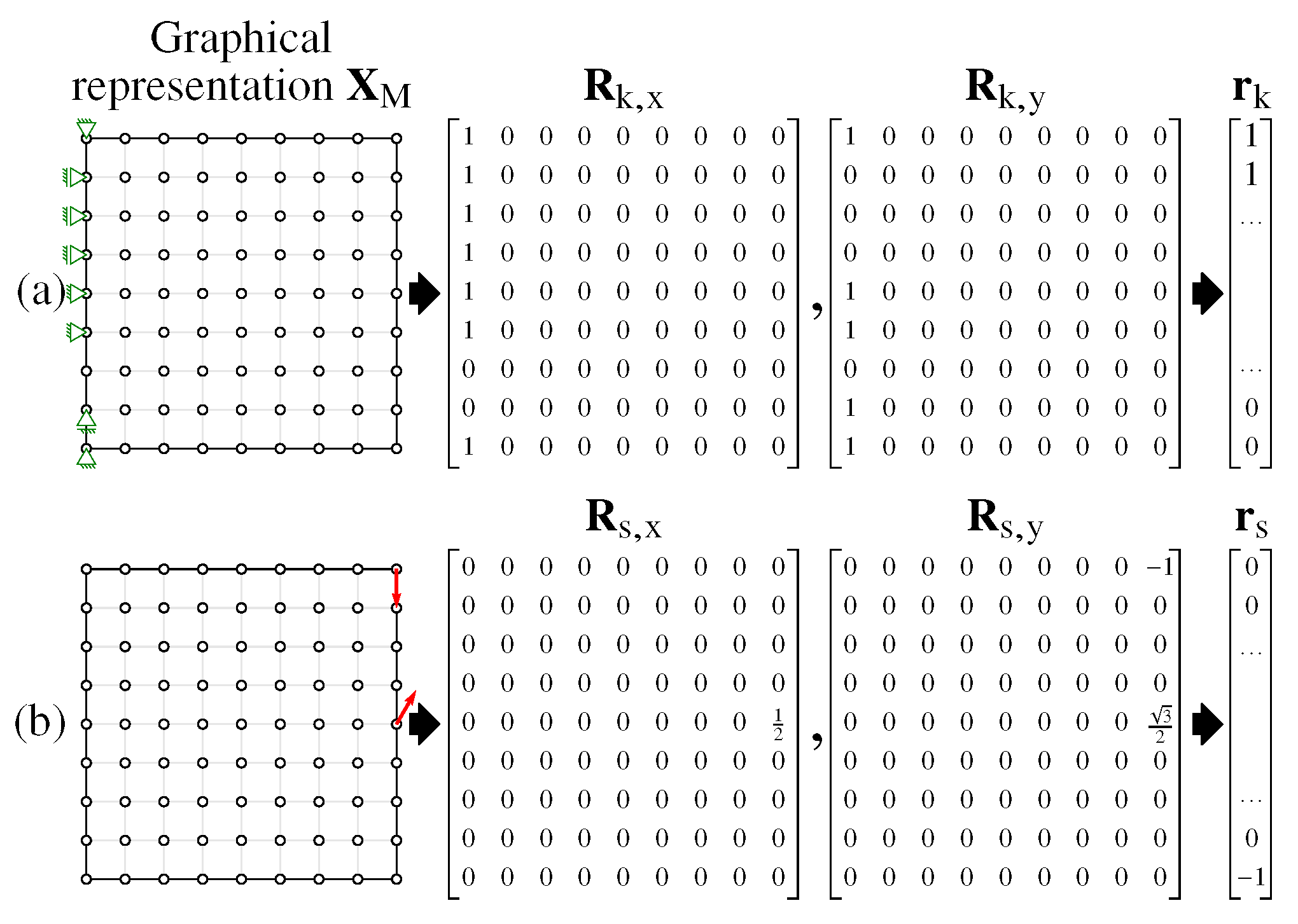
Figure 3 shows an overview of the processing of boundary conditions. In this figure as well as in following figures, the symbols represent the kinematic boundary conditions (structural supports) and the vectors of the static boundary conditions (applied forces).

Figure 3.
Matrix representation of (a) kinematic boundary conditions (structural supports) and (b) static boundary conditions (applied forces).
The kinematic boundary conditions are stored in two Boolean matrices and . The entries of are set to one if the x-component of the displacement in the corresponding node is fixed, and to zero otherwise. Analogously, the entries of are set according to the fixed y-components of the displacements. Both matrices can be transformed into vectors with the operator, which is the inverse of the operator , and then arranged in sequence so that the vector is created.
Analogous to the kinematic boundary conditions, two matrices and are firstly built on the basis of the static boundary conditions. The x- and the y-components of the applied forces are placed, respectively, into the matrices in correspondence to their magnitude, while the remaining entries are set to zero. The matrices and are then converted into the vector .
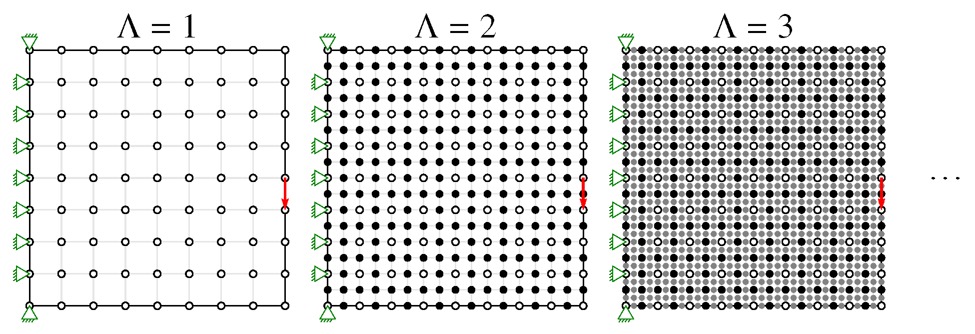
Investigations showed that the training speed could be increased, for high-resolution geometries, by dividing the training into levels with increasing resolution. Since smaller geometries are trained several orders of magnitude faster and the knowledge gained is also used for higher resolution geometries, the overall training time is reduced, compared to the training that uses only high-resolution geometries. The levels are labeled with the integer number .
Increasing by 1 results in doubling the number d of rows or columns of the design domain’s mesh. This is done by quartering the elements of the previous level. In this way, the nodes of the previous level are kept in the new level. The number of row or columns at the first level is denoted as .
The input data of the predictor include the kinematic and static boundary conditions as well as the target degree of filling . The output of the predictor is vector , which consists of the individual degree of filling values for each element. Input data can be only defined at the initial level and do not change when the level is changed. Hence, new nodes cannot be subject to static or kinematic boundary conditions (see Figure 4). When the level is changed, only the dimension of the outputs changes; the dimension of the inputs remains constant. The change in level occurs after a certain condition—which will be described later—is fulfilled.

Figure 4.
Nodes and elements at different levels (resolutions). The boundary conditions do not change.
2.2. Predictor
The predictor is responsible for generating the optimized result for a given input data point. Its ANN-architecture consists of multiple hidden layers, convolutional layers and output layers (see Figure 5).

Figure 5.
Predictor’s artificial neural network (ANN) topology (simplified).
All parameters that can be changed during training, such as the bias, the slope of the parametric rectified linear unit (PReLU) as well as the weights of the hidden layers, are generally referred to as trainable parameters in the following. They are collected in the matrix . The operations performed by the predictor can be represented by function as follows:
The predictor’s topology is shown in Figure 5 in a simplified form. An input data point (top left) is processed by several successive hidden blocks and then passed on to some residual network (ResNet)-blocks. In order to reduce the resolution to a lower level , average pooling is used.
In Figure 5, the hidden block is the combination of a hidden or fully connected layer and an activation function call. The ResNet-block is the combination of two (convolutional) layers and a shortcut that is added as a bypass to the output of the layers. The ResNet-block allows for faster learning but also reduces the error [27].
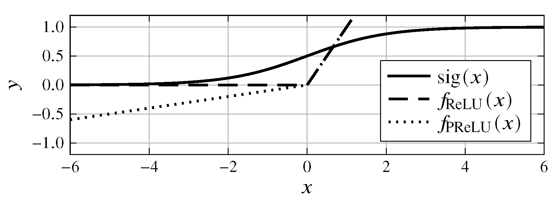
The PReLU function [28] is used as the activation function in the hidden and convolutional layers. The PReLU function is the equivalent of the rectified linear unit (ReLU) function [28]:
with the difference of a variable negative slope , which can be adapted during training as follows:
The sigmoid function
is well suited as an activation function for the output layer because it provides results in the interval (0,1); see Figure 6. This makes the predictor’s output directly suitable to describe the density values of the geometry.

Figure 6.
Sigmoid, ReLU and PReLU activation functions.
2.3. Evaluator: Compliance
The task of the compliance evaluator is the computation of the global mean compliance. For this purpose, an algorithm based on finite element method (FEM) [26] is used. The global mean compliance
is defined according to [26] as follows:
where is the stiffness matrix, is the force vector and is the displacement vector. The compliance has the dimension of energy. As is usual in [26,29], in the following, the units will be omitted for the sake of simplicity.
As already explained, the static boundary conditions vector consists first of x-entries and then y-entries. Since the degrees of freedom of the stiffness matrix are arranged in an alternate way (one x-entry and one y-entry), the force vector is to be built accordingly. In order to transform the static boundary condition vector into the force vector , the number of nodes
and a collocation matrix
are required. The force vector is then obtained as follows:
The system’s equation is as follows:
The stiffness matrix depends linearly on the geometry and is expressed by the following:
where the matrices are the unscaled contributions of the single elements to the stiffness matrix. The penalization exponent p achieves the desired focusing of the geometry toward the limits of values and 1 as described in Section 2.1.
The stiffness matrix is then reduced by removing the columns and rows corresponding to the fixed degrees of freedom according to the kinematic boundary conditions. The result is the reduced stiffness matrix , which then can be inverted. The reduced force vector is determined according to the same principle. From the reduced equation,
the reduced displacement vector is obtained as follows:
2.4. Evaluator: Degree of Filling
The task of this evaluator is to determine the deviation of the degree of filling (see (6)) from the target value as follows:
By considering the filling degree’s deviation M in the objective function, the predictor is penalized proportionally to the extent of the deviation from the target degree of filling .
2.5. Evaluator: Filter
The filter evaluator searches for checkerboard patterns in the geometry and outputs a scalar value that points to the amount and extent of checkerboard patterns detected. These checkerboard patterns consist of alternating high and low density values of the geometry. They are undesirable because they do not reflect the optimal material distribution and are difficult to transfer to real parts. These checkerboard patterns exist due to bad numerical modeling [30].
Several solutions for the checkerboard problem were developed in the framework of conventional topology optimization [31]. In this work, a new strategy was chosen, which allows for inclusion of the checkerboard filter into the quality function. In the present approach, checkerboard patterns are admitted but detected and penalized accordingly. Since the type of implementation is fundamentally different, it is not possible to compare the conventional filter method with the filter evaluator. With the matrix
the following two-dimensional convolution operation (discrete convolution) is performed:
In detail, the convolution operation is carried out as follows:
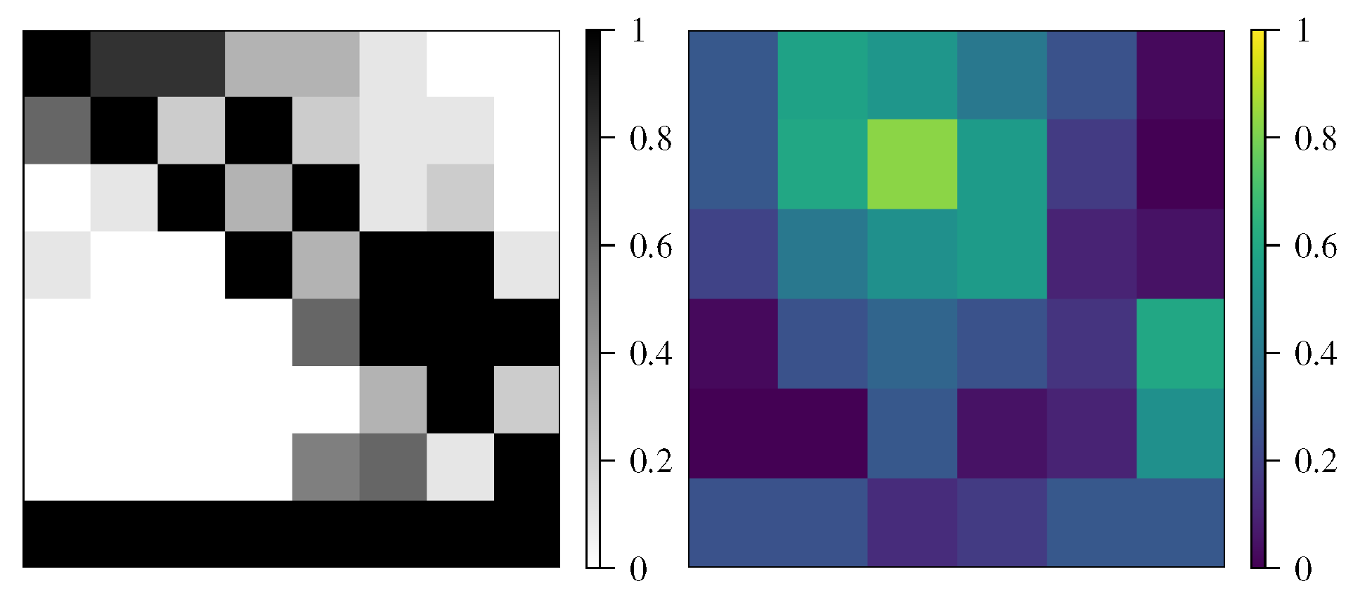
The convolution matrix is visualized in Figure 7 for an exemplary case.

Figure 7.
(Left): sample geometry. (Right): intermediate result (convolutional matrix ) in the checkerboard pattern search.
The matrix has high values in areas where the geometry has checkerboard patterns. A first indicator can be computed as the mean value of the convolution matrix:
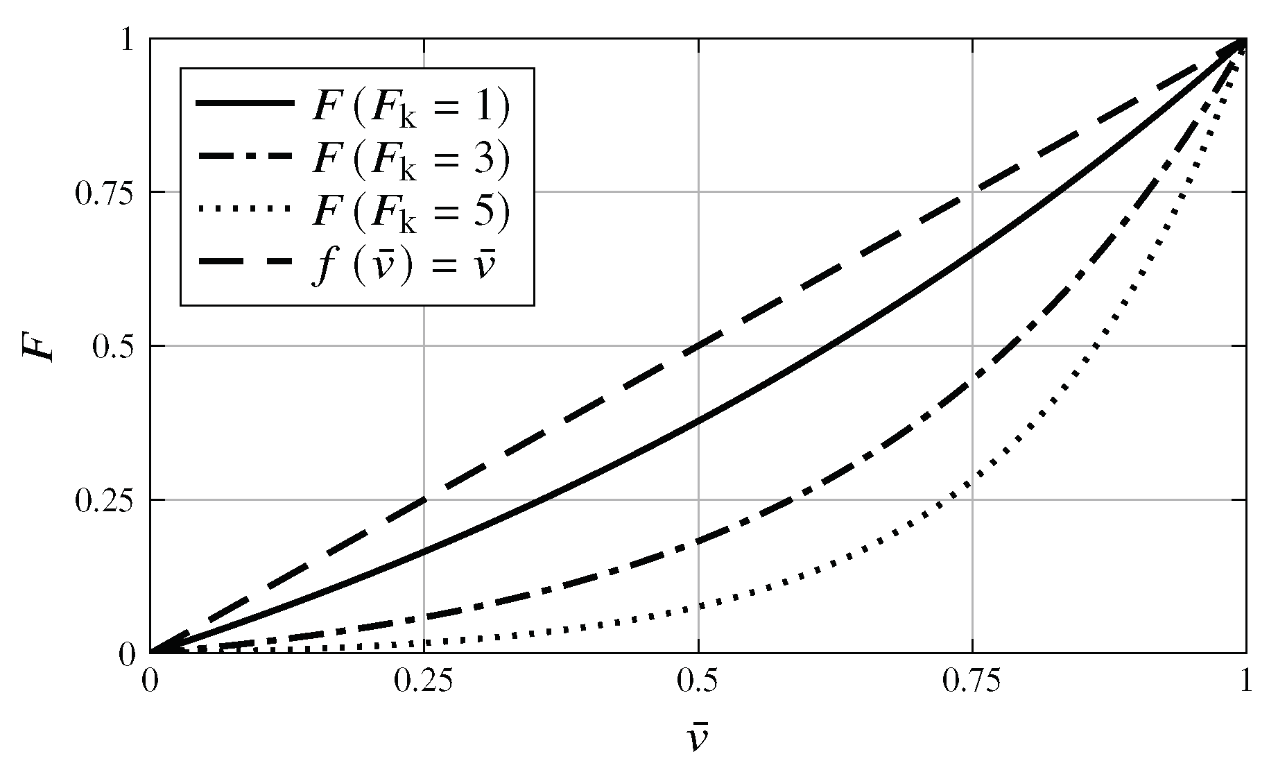
This indicator would already be sufficient to exclude geometries with checkerboard patterns but also penalizes good geometries without recognizable checkerboard patterns. Therefore, an improved indicator is formed on the basis of the mean value and with the help of the e-function, which is less sensitive to small mean values but nevertheless results in a corresponding penalization for large checkerboard patterns:
where the parameter controls the shape of the F-function (see Figure 8).

Figure 8.
Influence of factor on filter calculation.
2.6. Evaluator: Uncertainty
When calculating the density values of the geometry , the predictor should, as far as possible, focus on the limit values and 1 and penalize intermediate values. The deviation from this goal is expressed by the uncertainty evaluator with the scalar variable P. This value increases if the predicted geometry deviates significantly from the limit values and thus penalizes the predictor. The uncertainty evaluator uses the normal distribution function as follows:
with as the variance and as the expected value. The expected value is set to , at which P should have the maximum. In order for P to be normalized (with the function should have the value 1), the normal distribution function is multiplied by the term as follows:
The resulting function is evaluated for all elements of the geometry. The mean value of the results provides the following uncertainty:
where the variance determines the width of the distribution function.
2.7. Quality Function and Objective Function
The task of the quality function is to combine all evaluator losses into one scalar. The following additional requirements must be considered:
- The function should have a simple mathematical form, in order to not complicate the minimum search.
- The function must be monotonically increasing with respect to the evaluators’ losses.
- The function contains coefficients to control the relative influence of the evaluators losses.
The most obvious variant fulfilling these criteria is a linear combination of the losses. The problem with this choice consists of the different and variable order of magnitude of the compliance loss with respect to the other losses. For a given choice of the coefficients, the relative influence of the losses changes for different parametrization and input data points. To avoid this drawback, a quality function in the following form is chosen:
The addition of the constant value prevents the quality function from being dominated by one loss when its value is close to zero.
For every single data point, one value of exists. Optimization on the basis of single data points would require a large computational effort and lead to instabilities of the training process (large jumps of the objective function output). Therefore, a given number of training data points (batch) is used, and the corresponding quality function values are combined in one scalar value, which works as an objective function for the optimization that rules the training. The value of the objective function
is calculated as the arithmetic mean of the quality function values obtained for the single training data points of the batch. Investigations showed that averaging the quality function outputs over numerous training data points stabilizes the training procedure. The disadvantage of this averaging is the possibility of forming prejudices, e.g., if one element is frequently present, then its frequency is also learned, even if the element’s contribution to stiffness is in some cases small or non-existent.
2.8. Training
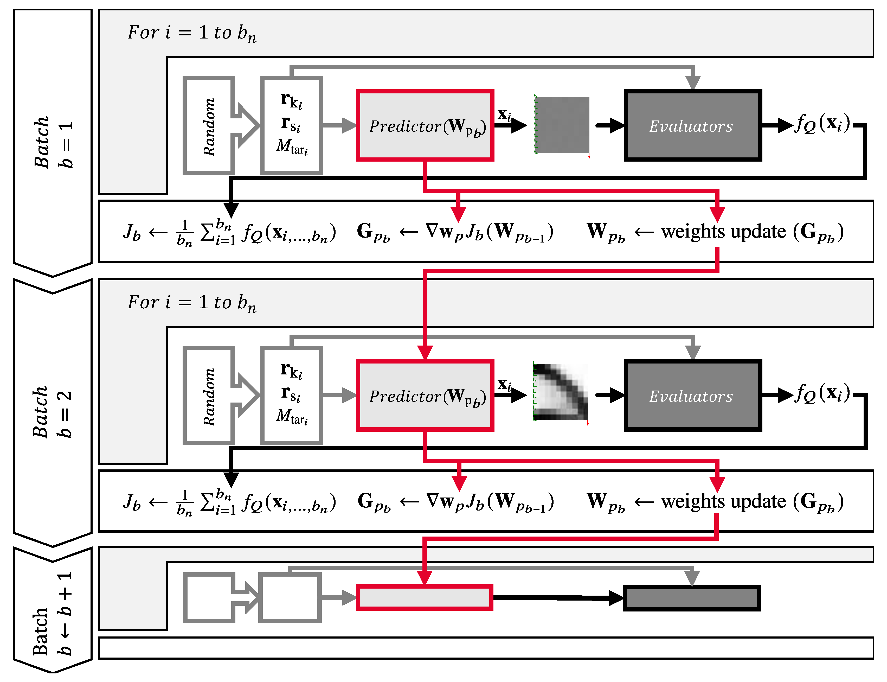
The overview in Figure 9 describes the training process for a single level. Here, it is visible that during a batch iteration, the input data points are calculated randomly and then passed to the predictor as well as to the evaluators.

Figure 9.
Training process of the predictor–evaluator network (PEN).
Within one batch, the input data points are randomly generated, and the predictor creates the corresponding geometries . Afterwards, the quality function is computed from the evaluators’ losses, according to (30). The objective function J is then calculated for the whole batch. Then, the gradient of the objective function, with respect to the trainable parameters, is calculated. The trainable parameters of the predictor for the next batch are then adjusted according to the gradient descent method to decrease the value of the objective function. In order to apply the efficient gradient descent method, the functions must be differentiable with respect to the trainable parameters [32]. For this reason, the evaluators and the objective function use only differentiable functions.
When the level increases, the predictor outputs a geometry with higher resolution, and the process starts again at batch .
It is important to stress that, unlike conventional topology optimization, the PEN method does not optimize the density values of the geometry, but only the weights of the predictor.
3. Application
3.1. Implementation
The implementation of the presented method takes place in the programming language Python. The framework Tensorflow with the Keras programming interface (API) is used. Tensorflow is developed by Google and is an open-source platform for the development of machine-learning applications [28]. In Tensorflow, the gradients necessary for the predictor learning are calculated using automatic differentiation (AD), which requires the use of differentiable functions available in Tensorflow [33]. The configuration of the software and hardware used for the training is shown in Table 1.

Table 1.
Configuration.
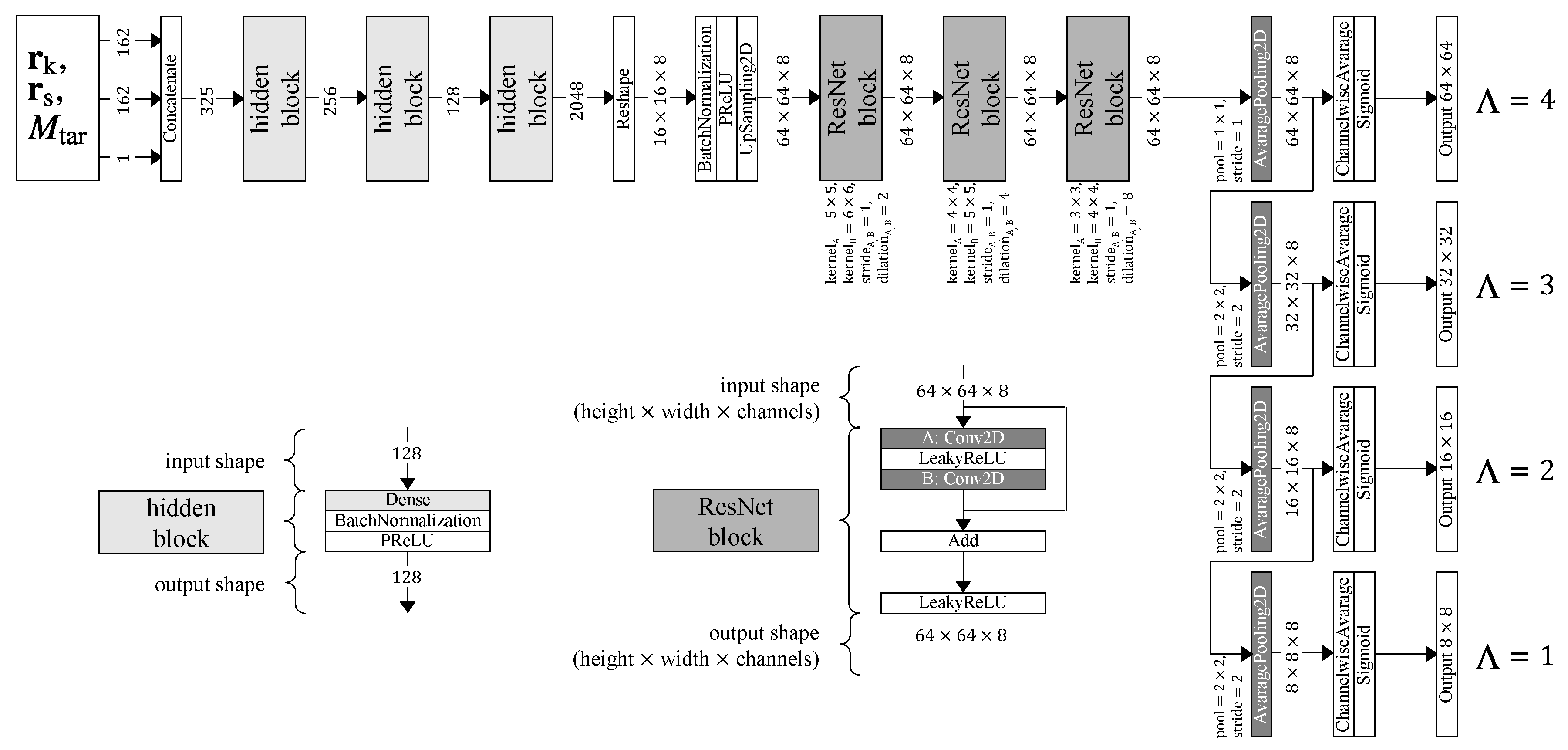
The predictor’s topology, with all layers and all hyperparameters, is shown in Figure 10. The chosen hyperparameters were found to be the best after a grid search of all parameters in which the deviations of the predictions from the ones obtained by conventional TO were evaluated. The hyperparameters are displayed by the shape (numerical expression over the arrow pointing outside the block) of the output matrix of a block or by the comment near the convolutional block. The label of the output arrow describes the dimensions of the output vector or matrix. The names of the elements in Figure 10, e.g., “Conv2D”, correspond to the Keras layer names.

Figure 10.
Predictor’s artificial neural network (ANN) topology.
The input data points (top left) are processed by four fully connected (here termed “dense”) layers, then reshaped into a three-dimensional matrix with the shape 8 × 8 × 64 and passed on to two sequential convolutional layers. Subsequently, the data are reshaped into a vector and passed through a sigmoid activation layer. As a result, the geometry at the first level is available. The following levels build on the previous levels. So the data from the last hidden block and the data prior to the sigmoid activation of the previous level are used by for the next layer by transforming the outputs to the same shape and adding them together. Afterwards, the data are reshaped into a vector and, again, passed through a sigmoid activation layer. As a result, the geometry at the next level is available.
As already mentioned, the training of the predictor is based on randomly generated input data points. All randomly chosen input data are uniformly distributed in the corresponding interval. They are generated according to the following features:
- Kinematic boundary conditions :
- –
- Fixed degrees of freedom along the left side in x and y directions.
- Static boundary condition :
- –
- Position randomly chosen from all nodes (except the nodes, which have a fixed degree of freedom) of level one.
- –
- Randomly chosen direction in the interval [0°,360°].
- –
- Fixed magnitude .
- Target degree of filling :
- –
- Uniform random .
Algorithms 1–3 show the training, the trainable parameter’s update and the convergence criterion, respectively.
The flow of data from the input of the ANN to the output and the objective function is called forward propagation.
With computation and updating of the objective function’s gradient with respect to the trainable parameters, the information flows backward through the ANN. This backward flow of information is called back-propagation [7]. Once the gradient is calculated, a trainable parameter’s update is done using the learning rate , which defines the length of the gradient step, and the Adam optimizer (see Algorithm 2), according to [32].
| Algorithm 1 Learning process, Part 1 (training) |
 |
| Algorithm 2 Learning process, Part 2 (trainable parameters update) | |
| ▹ gradients of objective function w.r.t. trainable parameters |
| ▹ rough estimation, for more details, see [32] |
After the trainable parameters of the predictor have been updated, a new batch can be elaborated. This process continues until a convergence criterion is fulfilled. In order to define a proper convergence criterion, the lowest objective function value in the current level is tracked and compared to the current objective function value . If the objective function value of one batch is not lower than , then the integer variable (patience) is increased by one—otherwise, it resets to zero:
Once the patience exceeds a predefined value , termed maximal patience (see Table 2), the level increases, or if the maximum level is reached, the training stops (see Algorithm 1 line 7).
| Algorithm 3 Learning process, Part 3 (convergence criterion) |
|
Table 2.
Parameter used for training and generation of validation data.
The values from Table 2 were used in the development of the method and in the generation of the validation data.
3.2. Results and Discussion
The training of the predictor lasted , which can be subdivided according to the individual levels as follows: 16%, 7%, 42%, 35%. The training processed approximately 7.6 million randomly generated training data points. The DL based TO geometries are similar to the results obtained by 88 lines of code (top88) according to [29] for the same input data points. Table 2 contains the parameters used for the conventional SIMP-TO density filter method. An example prediction is shown in Figure 11. The left result was obtained by the PEN method, and the right result was calculated by the conventional TO (88 lines of code) method under the same boundary conditions.

Figure 11.
Sample geometry (Left): deep learning-based topology optimization by using the predictor–evaluator network (PEN) method. (Right): 88 lines of code Andreassen et al. [29].
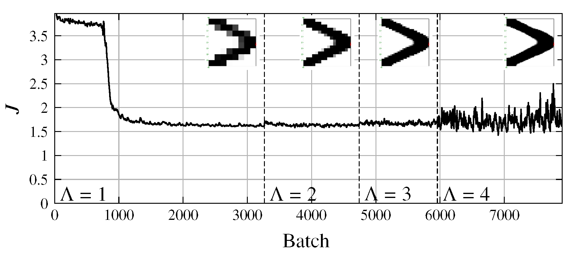
The training history shows the progression of the objective function (see Figure 12) and of the individual evaluator losses over the number of batches (see Figure 13). The smaller batch size at higher levels produces more oscillation of the curve and therefore, makes it difficult to identify a trend. For this reason, the curves shown in the figures are filtered, using the exponential moving average and a constant smoothing factor of 0.873 [34] for all levels. This filtering does not affect the original objective function and serves only visual purposes.

Figure 12.
Progression of the objective function value during training.

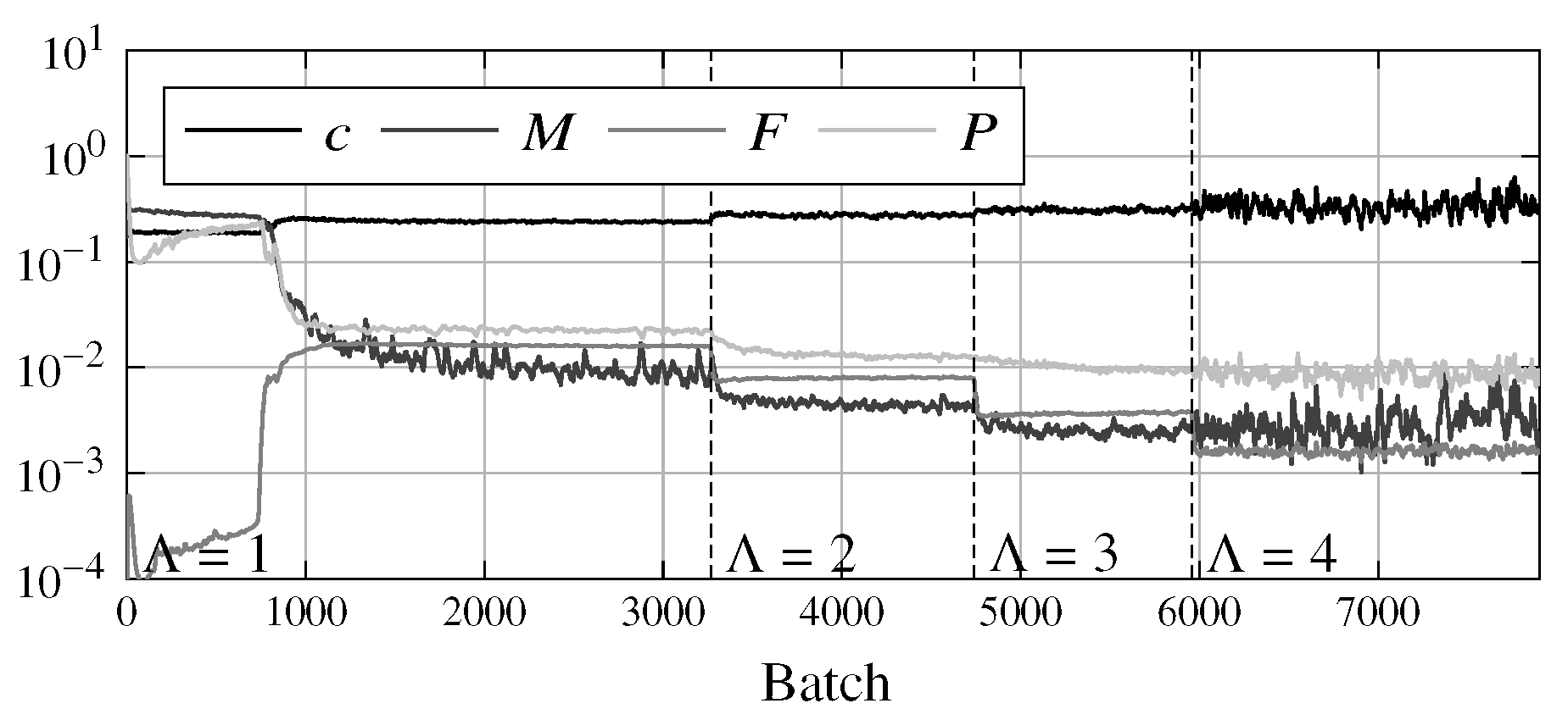
Figure 13.
Progression of the evaluator values during training.
The dashed vertical lines (labeled with the value of ) in Figure 12 and Figure 13 indicate the change in level. It can be seen that the objective function value J improves significantly in the first level and in the following levels only slightly. The reason for this is that learning in one level optimizes the resolution in subsequent levels as well. This is also the explanation for the fact that the objective function value hardly increases when a level is increased. A slight increase can nevertheless be seen, which is due to the increased resolution and thus, the higher number of evaluated elements and the increase in complexity.
The results were validated using randomly generated input data points, called validation data. These data points were not part of the training. The corresponding optimized geometries were conventionally calculated by the top88 algorithm.
The results of the comparison (PEN and top88) of the 100 validation data points are summarized in the plots in Figure 14.

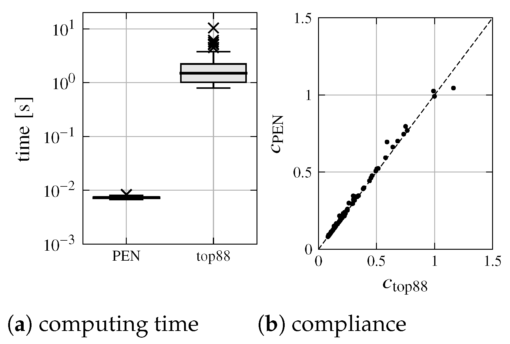
Figure 14.
Computing time and compliance comparison.
On average, the ANN-based TO can deliver almost the same result as the conventional method in about 7.3 ms, while the conventional topology optimizer according to Andreassen et al. [29] requires, on average, 1.9 s (and is, therefore, roughly 259 times slower); see Figure 14a. It can also be seen that the majority of geometries generated by PEN have a compliance that is close to the geometries generated by top88; see Figure 14b.
In addition to the comparison of compliance and computing time, there are indicators that allow the comparison of geometries generated by ANN-based TO with geometries generated by conventional TO.
The accuracy represents the conformity of the predicted geometries with the geometries of the validation data points. To determine the deviation of a single validation geometry xv from the predicted geometry xp, obtained from the same input data points, the following functions are used:
and
where n represents the number of validation data points and, in this case, has the value 100. The smaller the mean squared error (mse) and mean absolute error (mae) values, the
better the similarity of the results. The function indicates the percentage of elements with density differences of less than or equal to 0.01 with respect to the density values of the validation geometries generated by the conventional TO. For the calculation of , the Heaviside step function is used as follows:
With the help of the function
the accuracy and thus, the validity of the predictor can be determined, and predictors with different hyperparameters can be compared. The function is needed because a single indicator is not sufficient to determine the accuracy of the predictor. So, it is possible that the accuracy is low and the errors mae and mse are also small at the same time. Since these error indicators concentrate on different kinds of differences, the average of those is a more meaningful indicator.
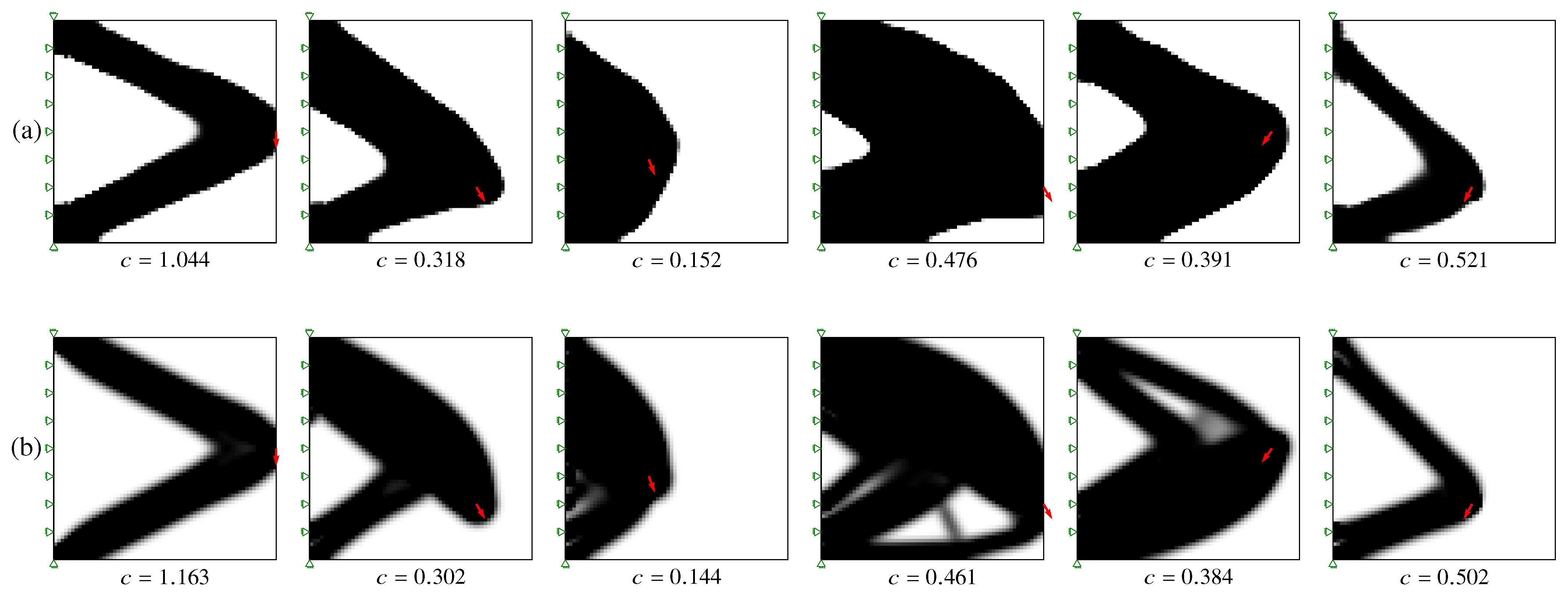
The examples in Figure 15 show that the predictor can deliver geometries that are similar to the conventional method, as well as some weaknesses. Unfortunately, the results are not always perfect, and some geometries lack details (see Figure 15, column four or five). This may be improved by an appropriate choice of layers or hyperparameters of the predictor and by adapting the quality function. For all sample geometries in Figure 15, the compliance is reported under the geometry diagram.

Figure 15.
Additional sample geometries: (a) generated with predictor–evaluator network (PEN); (b) conventionally generated validation data.
For the PEN-generated geometries, the evaluator losses are summarized in Table 3. It can be seen that the values for all evaluators—except the compliance evaluator—are close to zero. The compliance can only be reduced to an optimal value, which cannot be decreased without adding more material. It should also be noted that the deviation in the degree of filling M is not exactly zero, unlike what is expected by the conventional method. This is due to the fact that there is no restriction, but only a penalty for deviation.
Table 3.
Summary of evaluator losses (same examples as in Figure 15).
Table 4 shows all kinds of indicators that represent the conformity of PEN-generated geometries with conventionally generated geometries, averaged over all 100 examples. SD is the standard deviation.
Table 4.
Summary of indicators.
From the data in the Table 4, it can be seen that in the examined cases, 79.9% of the elements of the geometries obtained with the PEN method have density differences of less than 1% as compared to the conventionally optimized geometries.
3.3. Computing Time Comparison
It was mentioned in Section 3.2 that the PEN method is orders of magnitude faster than top88. However, the predictor profits from a computationally intensive training. So it is interesting to attempt a comparison which takes into account the training time.
The PEN computing time for a single geometry tPEN, including its share of training time, obviously depends from the number of geometries predicted ep on the basis of one single training process:
where tp is the computing time per single geometry and Tp is the training time. The break-even point (BEP) is given by the number of predictions eBEP for which both methods require the same time (including training time contribution). To calculate the BEP tPEN is set equal to tTO, which is the computing time to optimize a single geometry using the conventional method. It results as follows:
Table 5 shows the computing times of the different methods as well as the BEP.
Table 5.
Time comparison of conventional and predictor–evaluator network (PEN) based methods at a resolution of 64 × 64.
When evaluating the results of this comparison, the following points should be considered:
- Due to the fact that , the BEP, for a given reference method, essentially depends on the training time.
- The training time in turn depends on the convergency condition. Within the framework of this project, an extensive study about the proper choice of the convergency criterion could not be made. The present choice allowed for good results. It can be expected that the training time could be reduced after a targeted study in this sense.
- Of course, the training time also depends on the hardware used for training. By using a high performance hardware, the training time, and thus, the BEP, can be strongly reduced without affecting the versatility of the method in everyday use.
- This comparison does not include a study of the effect of the problem size (number of design variables).
3.4. Interactivity
Due to the ability to quickly obtain the optimized geometry by the predictor, the ANN-based TO can be executed interactively in the browser. Under the address: https://www.tu-chemnitz.de/mb/mp/forschung/ai-design/TODL/ (accessed on 23 September 2021), it is possible to perform investigations with different degrees of filling as well as static boundary conditions.
4. Conclusions
In this work, a method was presented to train an ANN using online deep learning and use it to solve optimization problems. In the context of the paper, TO was chosen as the problem to be solved. The ANN in charge of generating topology-optimized geometries does not need any pre-optimized data for the training. The generated geometries are, in most cases, very similar to the results of conventional topology optimization, according to Sigmund or Andreassen et al.
This topology optimizer is much faster, due to the fact that the computing-intensive part is shifted into the training. After the training, the artificial neural network based topology optimizer is able to deliver geometries that are nearly identical to the ones generated by conventional topology optimizers. This is achieved by using a new approach: the predictor–evaluator network (PEN) approach. PEN consists of a trainable predictor that is in charge of generating geometries, and evaluators that have the purpose of evaluating the output of the predictor during the training.
The method was tested for the 2D case up to an output resolution of 64 × 64. This choice is not a limitation of the method and can be improved by using better hardware for training or by high-performance computing. The use of the method for the 3D case and higher resolutions is conceivable. The optimization of the computational efficiency of the training phase was not the first priority of this project since the training is performed just once and, therefore, affects the performance of the method only in a limited fashion. A critical step is the calculation of the displacements in the compliance evaluator. The use of faster algorithms (e.g., sparse solvers) could remove the mentioned limitations. One approach to improve the learning process would be to train only in areas where there is a high potential for improvement, through appropriate selection of training data points.
The results of the PEN method are comparable to the ones of the conventional method. However, the PEN method could prove superior in handling applications and optimization problems of higher complexity, such as stress limitations, compliant mechanisms and many more. This expectation is related to the fact that no optimized data are needed. All methods that process pre-optimized data suffer from the difficulties encountered by conventional optimization, while managing the above-mentioned problems. Because the PEN method works without optimized data, it could also be applied to problems that have no optimal solutions or solutions that are hard to calculate, such as the fully stressed truss optimization.
To date, variable kinematic boundary conditions have not been tested. This will be done in future research, together with resolution improvement and application to three-dimensional design domains and different optimization problems.
Author Contributions
Conceptualization, A.H. (Alex Halle); data curation, A.H. (Alex Halle); formal analysis, A.H. (Alex Halle) and L.F.C.; investigation, A.H. (Alex Halle); methodology, A.H. (Alex Halle); project administration, A.H. (Alex Halle) and A.H. (Alexander Hasse); resources, A.H. (Alex Halle) and L.F.C.; software, A.H. (Alex Halle); supervision, A.H. (Alexander Hasse); validation, A.H. (Alex Halle); visualization, A.H. (Alex Halle); writing—original draft, A.H. (Alex Halle); writing—review & editing, A.H. (Alex Halle), L.F.C. and A.H. (Alexander Hasse). All authors have read and agreed to the published version of the manuscript.
Funding
The publication of this article was funded by Chemnitz University of Technology.
Institutional Review Board Statement
Not applicable.
Informed Consent Statement
Not applicable.
Data Availability Statement
The download of the predictor model as well as the validation data are publicly available at http://dx.doi.org/10.17632/459f33wxf6 (accessed on 23 September 2021).
Conflicts of Interest
The authors declare no conflict of interest.
References
- Sigmund, O.; Maute, K. Topology Optimization Approaches: A Comparative Review. Struct. Multidisc Optim. 2013, 48, 1031–1055. [Google Scholar] [CrossRef]
- Bendsøe, M.P.; Sigmund, O. Topology Optimization: Theory, Methods, and Applications; Springer: Berlin, Germany; New York, NY, USA, 2003. [Google Scholar]
- Aulig, N. Generic Topology Optimization Based on Local State Features; VDI Verlag: Dusseldorf, Germany, 2017; Volume 468. [Google Scholar]
- Picelli, R.; Townsend, S.; Brampton, C.; Norato, J.; Kim, H.A. Stress-Based Shape and Topology Optimization with the Level Set Method. Comput. Methods Appl. Mech. Eng. 2018, 329, 1–23. [Google Scholar] [CrossRef]
- Lee, E. Stress-Constrained Structural Topology Optimization with Design-Dependent Loads. Ph.D. Thesis, University of Toronto, Toronto, ON, Canada, 2012. [Google Scholar]
- Karayiannis, N.B.; Venetsanopoulos, A.N. Artificial Neural Networks: Learning Algorithms, Performance Evaluation, and Applications; Number SECS 209 in the Kluwer International Series in Engineering and Computer Science; Kluwer Academic: Boston, MA, USA, 1993. [Google Scholar]
- Goodfellow, I.; Bengio, Y.; Courville, A. Deep Learning; The MIT Press: Cambridge, MA, USA, 2016. [Google Scholar]
- Albawi, S.; Mohammed, T.A.; Al-Zawi, S. Understanding of a Convolutional Neural Network. In Proceedings of the 2017 International Conference on Engineering and Technology (ICET), Antalya, Turkey, 21–23 August 2017; pp. 1–6. [Google Scholar] [CrossRef]
- Basheer, I.; Hajmeer, M. Artificial Neural Networks: Fundamentals, Computing, Design, and Application. J. Microbiol. Methods 2000, 43, 3–31. [Google Scholar] [CrossRef]
- Yu, Y.; Hur, T.; Jung, J.; Jang, I.G. Deep Learning for Determining a Near-Optimal Topological Design without Any Iteration. Struct. Multidisc Optim. 2019, 59, 787–799. [Google Scholar] [CrossRef] [Green Version]
- Rawat, S.; Shen, M.H.H. A Novel Topology Optimization Approach Using Conditional Deep Learning. arXiv 2019, arXiv:1901.04859. [Google Scholar]
- Sasaki, H.; Igarashi, H. Topology Optimization Accelerated by Deep Learning. IEEE Trans. Magn. 2019, 55, 1–5. [Google Scholar] [CrossRef] [Green Version]
- Malviya, M. A Systematic Study of Deep Generative Models for Rapid Topology Optimization. engrXiv 2020. [Google Scholar] [CrossRef]
- Abueidda, D.W.; Koric, S.; Sobh, N.A. Topology Optimization of 2D Structures with Nonlinearities Using Deep Learning. Comput. Struct. 2020, 237, 106283. [Google Scholar] [CrossRef]
- Ates, G.C.; Gorguluarslan, R.M. Two-Stage Convolutional Encoder-Decoder Network to Improve the Performance and Reliability of Deep Learning Models for Topology Optimization. Struct. Multidisc Optim. 2021. [Google Scholar] [CrossRef]
- Behzadi, M.M.; Ilies, H.T. GANTL: Towards Practical and Real-Time Topology Optimization with Conditional GANs and Transfer Learning. arXiv 2021, arXiv:2105.03045. [Google Scholar]
- Goodfellow, I.J.; Pouget-Abadie, J.; Mirza, M.; Xu, B.; Warde-Farley, D.; Ozair, S.; Courville, A.; Bengio, Y. Generative Adversarial Networks. arXiv 2014, arXiv:1406.2661. [Google Scholar] [CrossRef]
- Zhang, Y.; Chen, A.; Peng, B.; Zhou, X.; Wang, D. A Deep Convolutional Neural Network for Topology Optimization with Strong Generalization Ability. arXiv 2019, arXiv:1901.07761. [Google Scholar]
- Nie, Z.; Lin, T.; Jiang, H.; Kara, L.B. TopologyGAN: Topology Optimization Using Generative Adversarial Networks Based on Physical Fields Over the Initial Domain. arXiv 2020, arXiv:2003.04685. [Google Scholar]
- Banga, S.; Gehani, H.; Bhilare, S.; Patel, S.; Kara, L. 3D Topology Optimization Using Convolutional Neural Networks. arXiv 2018, arXiv:1808.07440. [Google Scholar]
- Yamasaki, S.; Yaji, K.; Fujita, K. Data-Driven Topology Design Using a Deep Generative Model. arXiv 2021, arXiv:2006.04559. [Google Scholar]
- Cang, R.; Yao, H.; Ren, Y. One-Shot Generation of near-Optimal Topology through Theory-Driven Machine Learning. arXiv 2019, arXiv:1807.10787. [Google Scholar] [CrossRef] [Green Version]
- Chandrasekhar, A.; Suresh, K. TOuNN: Topology Optimization Using Neural Networks. Struct. Multidisc Optim. 2020. [Google Scholar] [CrossRef]
- Sosnovik, I.; Oseledets, I. Neural Networks for Topology Optimization. arXiv 2017, arXiv:1709.09578. [Google Scholar] [CrossRef] [Green Version]
- Qian, C.; Ye, W. Accelerating Gradient-Based Topology Optimization Design with Dual-Model Artificial Neural Networks. Struct. Multidisc Optim. 2020. [Google Scholar] [CrossRef]
- Sigmund, O. A 99 Line Topology Optimization Code Written in Matlab. Struct. Multidisc Optim. 2001, 21, 120–127. [Google Scholar] [CrossRef]
- He, K.; Zhang, X.; Ren, S.; Sun, J. Deep Residual Learning for Image Recognition. arXiv 2015, arXiv:1512.03385. [Google Scholar]
- Abadi, M.; Agarwal, A.; Barham, P.; Brevdo, E.; Chen, Z.; Citro, C.; Corrado, G.S.; Davis, A.; Dean, J.; Devin, M.; et al. TensorFlow: Large-Scale Machine Learning on Heterogeneous Distributed Systems. arXiv 2015, arXiv:1603.04467. [Google Scholar]
- Andreassen, E.; Clausen, A.; Schevenels, M.; Lazarov, B.S.; Sigmund, O. Efficient Topology Optimization in MATLAB Using 88 Lines of Code. Struct. Multidiscip. Optim. 2011, 43, 1–16. [Google Scholar] [CrossRef] [Green Version]
- Díaz, A.; Sigmund, O. Checkerboard Patterns in Layout Optimization. Struct. Optim. 1995, 10, 40–45. [Google Scholar] [CrossRef]
- Sigmund, O.; Petersson, J. Numerical Instabilities in Topology Optimization: A Survey on Procedures Dealing with Checkerboards, Mesh-Dependencies and Local Minima. Struct. Optim. 1998, 16, 68–75. [Google Scholar] [CrossRef]
- Kingma, D.P.; Ba, J. Adam: A Method for Stochastic Optimization. arXiv 2017, arXiv:1412.6980. [Google Scholar]
- Baydin, A.G.; Pearlmutter, B.A.; Radul, A.A.; Siskind, J.M. Automatic Differentiation in Machine Learning: A Survey. arXiv 2015, arXiv:1502.05767. [Google Scholar]
- Nicolas, P.R. Scala for Machine Learning, 2nd ed.; Packt Publishing, Limited: Birmingham, UK, 2017. [Google Scholar]


Publisher’s Note: MDPI stays neutral with regard to jurisdictional claims in published maps and institutional affiliations. |
© 2021 by the authors. Licensee MDPI, Basel, Switzerland. This article is an open access article distributed under the terms and conditions of the Creative Commons Attribution (CC BY) license (https://creativecommons.org/licenses/by/4.0/).