Deep Representation of a Normal Map for Screen-Space Fluid Rendering

Abstract

We propose a novel method for addressing the problem of efficiently generating a highly refined normal map for screen-space fluid rendering. Because the process of filtering the normal map is crucially important to ensure the quality of the final screen-space fluid rendering, we employ a conditional generative adversarial network (cGAN) as a filter that learns a deep normal map representation, thereby refining the low-quality normal map. In particular, we have designed a novel loss function dedicated to refining the normal map information, and we use a specific set of auxiliary features to train the cGAN generator to learn features that are more robust with respect to edge details. Additionally, we constructed a dataset of six different typical scenes to enable effective demonstrations of multitype fluid simulation. Experiments indicated that our generator was able to infer clearer and more detailed features for this dataset than a basic screen-space fluid rendering method. Moreover, in some cases, the results generated by our method were even smoother than those generated by the conventional surface reconstruction method. Our method improves the fluid rendering results via the high-quality normal map while preserving the advantages of the screen-space fluid rendering methods and the traditional surface reconstruction methods, including that of the computation time being independent of the number of simulation particles and the spatial resolution being related only to image resolution.

1. Introduction

Particle-based methods are often used for fluid simulation, and many rendering methods have been developed for drawing high-quality particle surfaces. Among the various particle rendering methods, screen-space-based methods [1] have been popular because of their ability to render particles in real-time with a configurable trade-off between speed and quality. However, screen-space-based methods have certain problems such as the surface appearing convex and cases where the front and back of a particle are not distinguishable. Some studies have proposed the use of alternative filters to address these problems [2], but these filters are not suitable for general use.

In screen-space-based methods, the normal map is crucially important because it determines the shape and color of the rendered results. The normal map is often created by filtering the particle data in the screen space. While considering screen-space rendering methods, we have been inspired by recent work in image generation using deep convolutional neural networks [3,4]. The state-of-the-art deep convolutional neural networks architecture has a trend targeting high performance. The trend lead a network architecture to more complex. Because our goal is implementation of the architecture having high cost-effectiveness, the state-of-the-art technique is not suitable. Therefore, we propose a deep learning method that generates a highly refined normal map for fluid rendering and is based on conditional generative adversarial networks (cGANs) [5]. The use of cGANs is a common aspect in a range of studies involving GANs [6]. To infer the probability distribution of the true data, a GAN trains a $generator$ and a $discriminator$ to solve a min-max problem. The discriminator is trained to distinguish the true data from data generated by the generator, and the generator is trained to “mislead” the discriminator. A cGAN leverages a GAN in a conditional setting that is not simply an approximation of the true data probability distribution but an inference of the conditional probability distribution. This makes cGANs suitable for image-to-image style translation tasks [4].

In this study, we consider the refinement of a normal map as an image-to-image style translation problem and employ a cGAN-based method for the outputs. Instead of smoothing the particle surface in the screen space using an existing approach, such as using a Gaussian blur or various filters, we train the cGAN generator as a filter to refine the low-quality normal map to produce a high-quality map, thereby improving the rendering results.

For the training process, a key issue is the construction of a training dataset that comprises pairs of low-quality and high-quality normal maps. To address this, we begin with a low-quality normal map created in the screen space by a 2D filter (bilateral Gaussian filter), which we call the “input normal map”. Then, the model uses the training process to refine the input normal map to resemble that generated by a 3D reconstructed surface [7]. We call the high-quality normal map extracted from the 3D reconstructed surface the “target normal map”. Having constructed such a normal map dataset for a variety of fluid simulation scenes, we demonstrated that use of the dataset could yield rendering results with clearer and more detailed features. In addition, we introduce a novel specialized loss term called the “normal constraint loss” for generative networks, which learns the constraints on the normal map. During the actual rendering, we first create a normal map in the screen space and then refine the normal map by inserting it into the previously trained deep learning model. Experiments demonstrated that our method can be effectively applied to an arbitrary fluid scene and can obtain satisfactory results (as shown in Figure 1).

There is a significant difference between the proposed method and existing particle rendering methods. Because the target normal map is generated using a surface reconstruction method, our method is more robust than the existing screen-space methods [1,2] with respect to preserving features in the rendering results. In addition, because the cGAN model generates a refined normal map through a convolution operation, the computation time is related neither to the number of particles nor to the resolution of the surface reconstruction method [7]. Owing to this characteristic, the rendering quality tends to be improved in some cases.

The contributions of the present study can be summarized as follows.

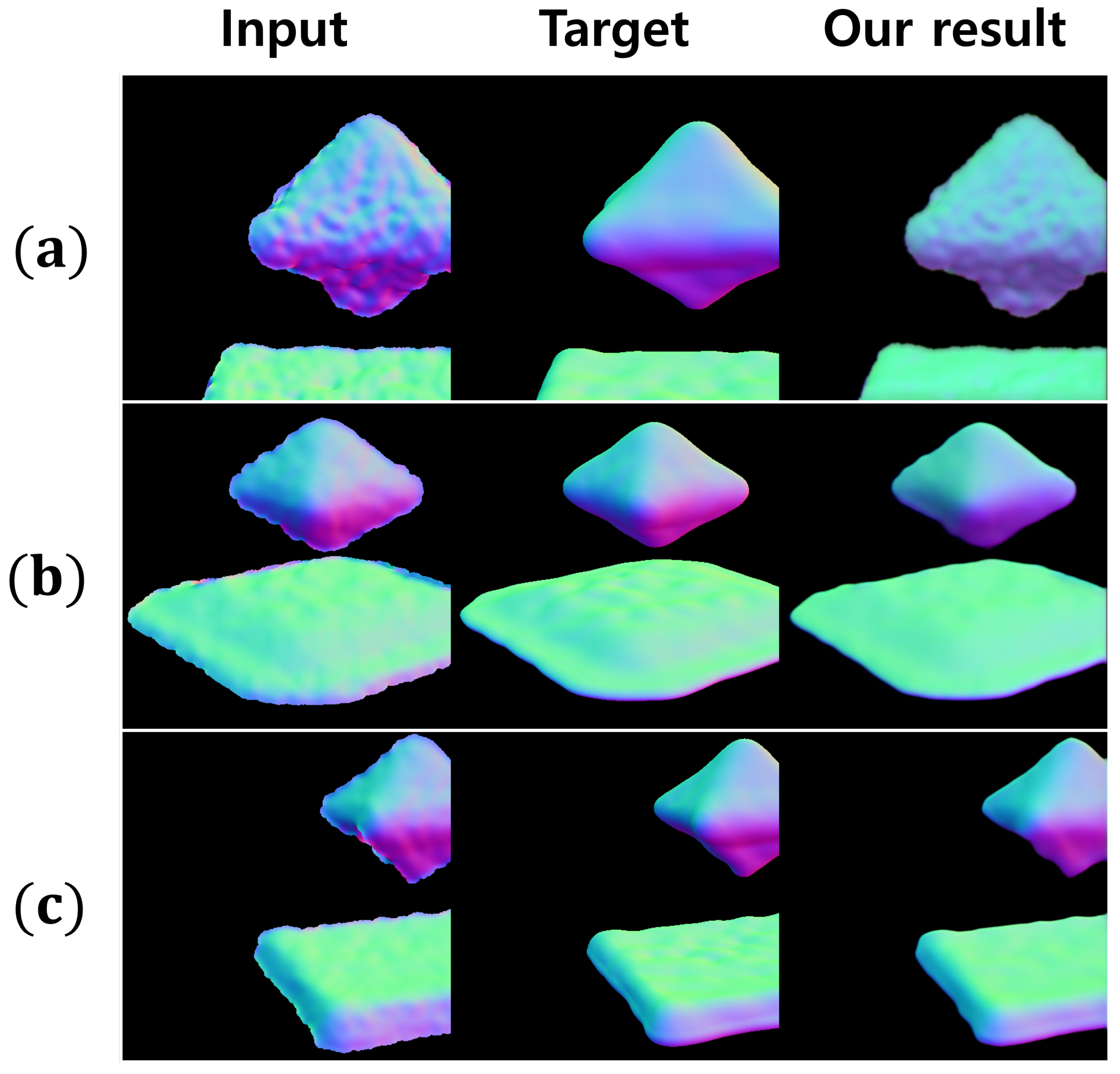
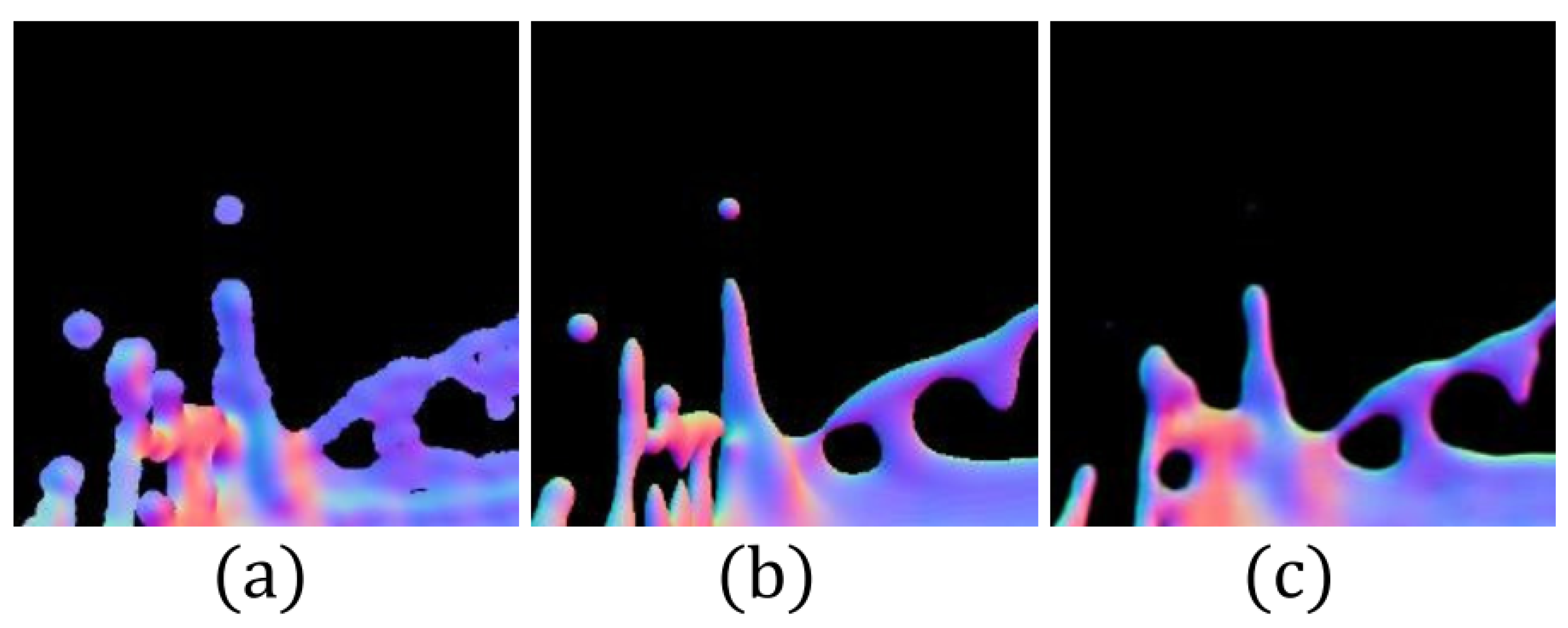
• We propose a cGAN-based filter to improve the results of screen-space fluid rendering effectively.
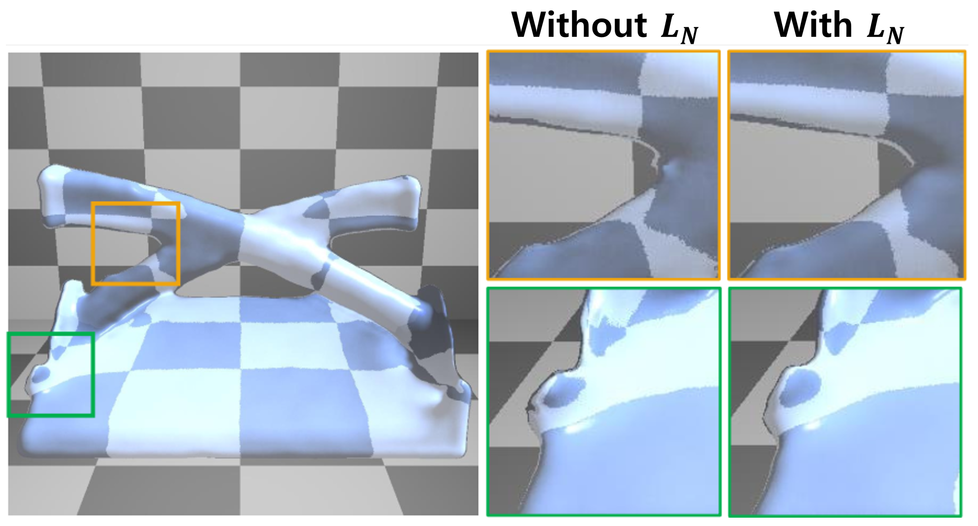
• We propose a novel loss term to encourage clear refinement of the normal map.
• Because we constructed a normal map dataset for different types of fluid simulation, the experimental results generated by the deep normal map representation demonstrated the generality of our method and its efficient applicability to arbitrary fluid scenes.

2. Related Work

Screen-space fluid rendering: There are many methods that can be used to render a particle-based fluid simulation, with the traditional method being the isosurface-based approach [7]. However, when an isotropic kernel is used to extract isosurfaces, all the particles are represented as spheres, which causes the surface of the fluid to appear rough. To address this problem, one study used an anisotropic kernel [8] to distribute nearby particles when the physical quantity at a certain point was obtained. When the anisotropic kernel is used, particles can be expressed as ellipsoids instead of spheres, which can solve the problem of surface roughness. However, the method of extracting and rendering isosurfaces requires a considerable amount of computation because the physical quantities must be calculated for each space.

Apart from creating a surface and rendering it in the world space, there are other approaches that extract and render particles in the screen space without creating a surface. Among the traditional methods, one method renders point clouds [9] and another renders fluid particles [1]. Here, a Gaussian filter [10] or a bilateral Gaussian filter is commonly used to smoothen the surface. However, when these filters are used, there is an problem in that discontinuities occur between the front and rear particles. One approach for resolving this problem uses a narrow filtering technique [2], and another, called “screen-space mesh” [11], combines the aforementioned two methods for rendering particles with a smooth surface. Finally, another method predicts the fluid surface using ray tracing alone [12] and generates the ray-traced image using both ray tracing and deep learning [13].

In these studies, the screen-space method has an advantage over other methods in terms of the computation time. However, the rendering quality of the screen-space method is primarily related to the quality of the normal map, and the existing filters do not achieve high-quality rendering results. Inspired by the screen-space rendering method, our study aims to generate an optimal deep learning-based filter for refining the normal map to achieve high-quality screen-space fluid rendering.

Deep learning techniques: Deep learning has attracted considerable attention in a variety of fields and has exhibited outstanding performance in certain areas. Image classification has evolved to the point where it can outperform humans [14], and deep learning is used in many fields, such as natural language processing [15] and image processing [16,17]. Deep learning has also been used in the field of rendering. For example, path-traced images with few samples have been denoised using an autoencoder [18], and one study examined the high-quality rendering of various shading effects by learning from example images [19]. Graph neural networks (GNN) [20,21], which have strong relational properties owing to their architecture that represents relations using a graph, were studied for simulating complex physical systems (fluid, cloth, hair, etc.). In recent years, GNNs have been extended for non-particle-based simulations such as mesh-based [22] and grid-based [23] simulations.

In addition, deep learning has made significant progress in creating a production model that generates data that are similar to real-life [24]. The GAN approach, a model introduced by Goodfellow et al. [6], creates a generation model using a generator to generate data and a discriminator to distinguish between the generated data and the actual data. The generator and discriminator compete to improve the overall performance of the generator. Zhu et al. [25] proposed a cycle-GAN method for translating two different styles of images. cGAN [5] was proposed as a method for generating data with GANs under specific conditions, and it is better suited to the image-to-image translation problem. Studies involving cGANs include research on the super-resolution problem [26,27] and the image-style transfer problem [28].

Inspired by these studies, our research adopts the cGAN method to generate an optimal deep-learning-based filter for refining the normal map to achieve high quality.

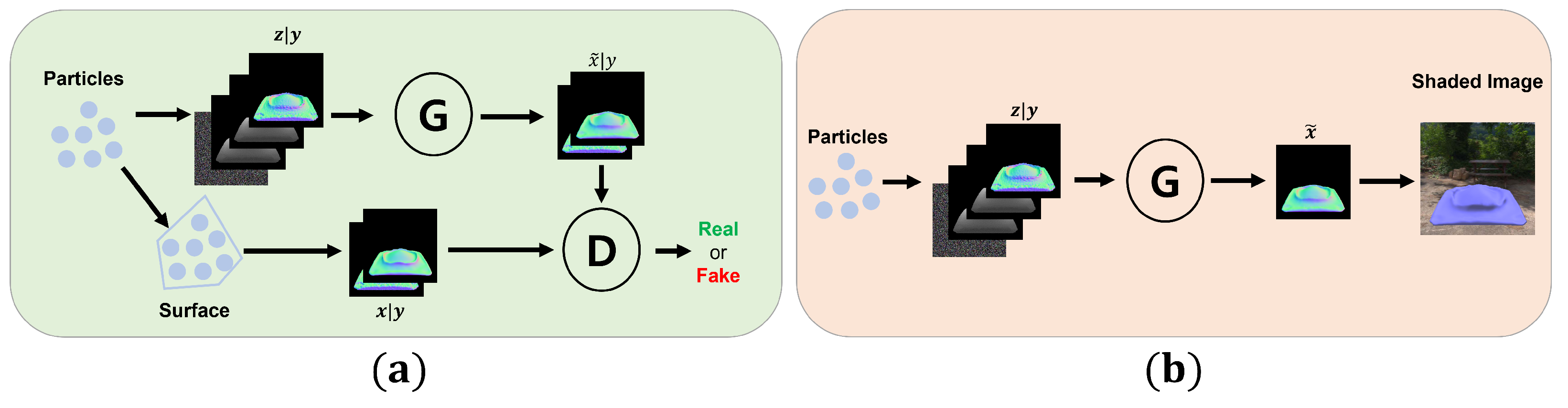
3. Deep Normal Map Representation with cGANs

Our method comprises two steps: training the deep learning model and performing fluid rendering based on the trained model (as shown in Figure 2).

In the first step, we train two networks: a generator G and a discriminator D. The cGAN learns a mapping from observed data y (including a screen-space normal map, a screen-space depth map, and a blurred screen-space depth map) and a typical random noise vector z to the target data, x (the normal map generated by the 3D reconstructed surface). Whereas the generator is trained to mimic the “real” normal map to mislead the discriminator, the discriminator is trained to judge the normal map generated by the generator as “fake” and the normal map generated by the 3D reconstructed surface as “real”. Because we want the generator to create a normal map based on the input data condition, the generator and discriminator both observe the screen-space normal map.

In the second step, we first create a depth map and a blurred depth map in accordance with the existing screen-space methods. Then, we create a normal map using the blurred depth map. The created normal map, a depth map, and a blurred depth map are given as the input data to the trained generator to create a new refined normal map. Finally, the refined normal map is used to calculate the lighting, reflection, and refraction for the final fluid rendering.

3.1. Conditional Generative Adversarial Networks

There are many the state-of-the-art neural network architecture having high performance but high cost in these day. However, because our target is the implementation of an architecture that is highly cost-effective, our method is based on the cGAN [5] for effective normal map refinement, where the objective function is

$$\begin{array}{c}\underset{G}{min}\underset{D}{max}V(D,G)=E_{x,y}\left[logD\left(x\right|y)\right]+E_{z,y}\left[log(1-D(y,G\left(z\right|y)))\right].\hfill \end{array}$$

(1)

Because generator G and discriminator D train for min-max optimization with value function $V(G,D)$, the generator outputs an image that is similar to the target image. Unlike unconditional GANs [6], G and D are both conditioned with respect to observed image y. G generates image $\tilde{x}$ according to the input noise vector, z, using information from observed image y. D takes either observed data y and generated data $\tilde{x}$ as the input or observed image y and target image x as the input; then, it evaluates the probability of the input image coming from the target image. D is trained to output 1 (“real”) for the target image pair or 0 (“fake”) for a generated image pair. Meanwhile, G is trained to encourage D to output 1 (“real”) for its generated image pair.

3.2. Normal Constraint Loss

To improve the generator’s performance, we propose a novel loss term called the “normal constraint loss”.

The normal map is a normal-vector-encoded image, and the normal data have the property that their lengths are one. We can perform a transformation that encodes the normal vector into image pixel data. First, we scale the vector by 0.5, add 0.5 for each element, and then multiply by 255 to yield element values in the range of 0 to 255. We denote the inverse of this transformation as N. For every pixel in the normal map to be decoded correctly, we use a $min$ function to help distinguish between the normal and empty positions via unit vectors and zero vectors, respectively, as follows:

$$L_N={\lambda }_{N}min(1-\parallel N\left(\tilde{x}\right){\parallel }_1,\parallel \tilde{x}{\parallel }_1).$$

(2)

Figure 3 presents examples of the optimization with and without normal constraint loss.

Empirically, loss functions $L1$ and $L2$ are commonly used with GAN-based methods to encourage G to create an image that resembles the target image [29]. We define the difference between the generated image and the target image for each pixel’s channel as a content loss and experiment with both $L1$ and $L2$ losses. However, our experiments and previous approaches [4,30] revealed that using the $L1$ loss instead of the $L2$ can lead to less blurring and fewer splotchy artifacts, as shown in Figure 4. Therefore, we adopt

$$L_C={\lambda }_C{\parallel \tilde{x}-x\parallel }_1.$$

(3)

Our final objective function can then be expressed as

$$G^{*}=\underset{G}{min}\underset{D}{max}V(D,G)+L_C\left(G\right)+L_N\left(G\right).$$

(4)

3.3. Rendering

After the cGAN training process is completed, we perform the rendering using the trained generator. Given the fluid particles’ positional data, we first create a normal map in the screen space using a bilateral Gaussian filter. To generate a result with clearer and more defined edges, we also create a depth map and a blurred depth map as inputs for the generator. The generator then generates the refined normal map that we use to render the final result. During the final rendering process, the convolution operation may cause some noise, which we remove by ignoring the pixels whose length is less than a threshold value. Examples of our rendering results are presented in Figure 1.

4. Training Data and Model Architecture

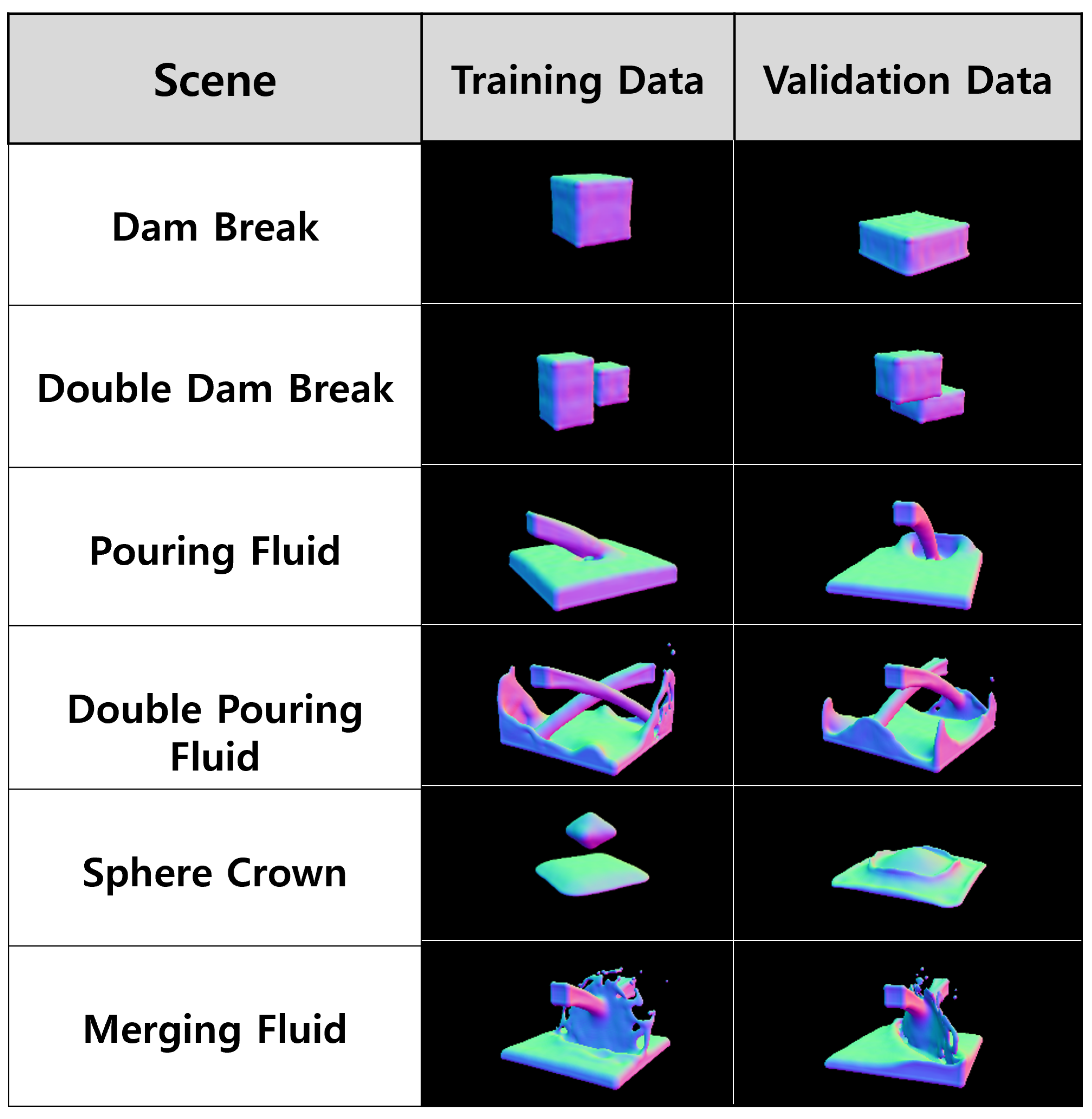
4.1. Datasets and Training Scenes

Now, we describe the preparation of the input and target training datasets. The input datasets were generated using a screen-space fluid rendering method based on a bilateral Gaussian filter. The target datasets were generated using the marching-cube method, which is a 3D surface reconstruction method that is used for particle data. We implemented the simulation of the fluid movement by adopting the smoothed particle hydrodynamics method [31,32]. Figure 5 presents examples of the training data.

Generating input datasets: The screen-space fluid rendering method is an existing method that is used to render particle data in a 3D space on a 2D screen. The basic idea is to map particles in the 3D space to a spherical point sprite on the 2D screen and blur the image to make it look like a fluid surface. First, the 3D object-space positions are transformed into 2D screen-space positions through projection, and a spherical point sprite is generated around the corresponding point. However, if we blur the spherical point sprite immediately, a problem is created. Suppose we create a virtual sphere with its center as the front and its edge as the back and use it to generate a depth map. Because the particles need to look like fluids, we smoothen the particle surface by blurring the depth map in the screen space. While blurring the depth map, only weighing the distance between pixels would not help in distinguishing between the front particles and the back particles. Therefore, we use a bilateral Gaussian filter, which also considers the depth value. In the blurred depth map, the normal direction is determined by the value of the differences between a pixel and its neighboring pixels. After the normal direction is determined, we encode the direction data into the normal map and perform deferred rendering using this generated normal map. However, because we assume every particle to be a sphere while generating the normal map, the surface appears bumpy, and the continuity between the front and back particle is not represented well. Moreover, because the filter size is fixed in the screen space, the resulting image is dependent on the distance between the camera and the particles.

Despite these artifacts, this method is most commonly used in scenes where the emphasis is on real-time processing because the computation speed is minimally related to the number of particles and can be accelerated using a GPU shader. In our experiments, a normal map generated using the screen-space method was used as part of the input data, with a bilateral Gaussian filter. To improve the finer details, the depth map and blurred depth map were also included in the input data.

Generating target datasets: The basic idea of the marching-cube approach is the creation of a triangle-shaped surface from the particle data. After the surface is created, its isosurface is extracted. First, we partition the simulation space, and the physical quantity assigned to each space (i.e., a scalar field) is calculated using the quantities assigned to each particle. The fluid surface is created by distinguishing the inside and outside of the fluid using a user-defined threshold.

Increasing the resolution to partition the space equally has the advantage of creating a smooth surface. In addition, if an anisotropic kernel is used to calculate the physical quantities assigned to a space, each particle is not generated as a simple sphere but as an ellipsoid, in accordance with the distribution of surrounding particles. When this approach is used, the computation time is increased, but a more water-like surface is created. The marching-cube method has a disadvantage in that the computation time depends on the spatial resolution and the number of particles because a scalar field must be calculated for each particle. Therefore, this method is not often used in real-time rendering, where the computation time is important.

In our experiments, a normal map generated using the marching-cube method was used for the target datasets. Because the surface creation time is independent of the computation time of our proposed algorithm, a marching-cube surface extraction algorithm with an anisotropic kernel was used.

While creating a normal map, the view-space normal was used, with every normal being a unit vector in the 3D space. Therefore, to store data in the range of 0∼1, each channel was multiplied by 0.5, and 0.5 was added.

Scene types: Several sets of training data were used to investigate the results obtained in a variety of situations (as shown in Figure 6). The training data comprised six scenes in total. The training data and validation data were generated separately for each scene. While training the model, we updated the weights using the training data and checked how the training was proceeding by using validation data at every epoch.

We simulated 500 frames for each scene. For each scene, there was a static scene where the camera was held as the motion of the fluid was rendered, and there was also a dynamic scene where the camera moved around as the fluid motion was rendered.

In the training process, we used cropped 512 × 512 images, applying data augmentation to increase the amount of data. This process was only applied to translation (not to rotation and shear) because the normal is defined in the view space, as shown in Figure 7.

4.2. Model Architecture

As shown in Figure 8(left), the generator contains convolution, deconvolution, activation, and batch normalization components. However, to prevent the problem of plaid patterns following deconvolution, we did not reverse the convolution and instead resized the data using a nearest-neighbor method; moreover, we used a same-size convolution. Batch normalization and Leaky ReLU [33] activation were applied to each convolution and deconvolution layer, and residual nets [34] were used. The auxiliary feature was used in conjunction with normal data in the first stage of the generator by using the contact operation. Because only the convolution layer is used rather than the fully connected layer at all stages, data can be processed at an arbitrary resolution after training.

As shown in Figure 8(right), the discriminator includes convolution, activation, and batch normalization components and a fully connected layer. We used the sigmoid activation function in the last layer to ensure output values in the range of 0∼1. As for the generator, batch normalization and Leaky ReLU activation were applied in the middle of each convolution operation. Screen-space normals were added to enable the discriminator to judge well.

An Adam optimizer [35] was used as the gradient descent method. The initial value of the learning rate was $0.0002$, which decreased as the training progressed. We define sampling as all the data that were sampled once in each epoch. Each training epoch was 100, and because of GPU memory limitations, we used a stochastic gradient descent that sampled only a part of the training data during the gradient descent. The batch size was set to 8. Because the training data were a continuous frame, we randomly shuffled it first. The training time was approximately four hours.

5. Experiments and Analysis

Our system was implemented using C++, Python, OpenGL, TensorFlow [36], and Boost Python. All the results were acquired using a standard PC with a 3.40 GHz i7-6700k CPU and an NVIDIA GeForce GTX 1080 graphics card. Now, we will discuss our results for the various datasets and for various parameter settings.

5.1. Auxiliary Features

As mentioned above, our model takes a normal map generated using the screen-space method as input and generates a highly refined normal map like a normal map generated using marching-cube method. Considering this, it is reasonable that only a normal map is used for training. However, recent deep learning-based research has reported that adopting auxiliary features for training improves training quality [37]. Accordingly, we introduced auxiliary features, including a depth map and a blurred depth map. To justify our choice, we investigated the effect of these auxiliary features.

Figure 9 presents the results obtained using the same parameters and conditions with and without the auxiliary features. The images were generated by our model after 100 training epochs with the same training dataset. Without the auxiliary features (depth and blurred depth), the results appear faint near the edges, and some noisy artifacts exist. Although adding only one auxiliary feature (depth or blurred depth) produced better results than the results obtained without either, we decided to add both features because the result was improved at the point where the particles are tapered.

We can hypothesize ways in which these auxiliary features can improve the training quality. The surface edge is typically generated when the distribution of the surface normal is diverse. However, there are some cases where the surface normal distribution is less varied (Figure 10). We assume that this is because the non-blurred depth map has a depth value in each pixel, and the surface edge can be improved (see the red circle in Figure 9). Because the blur method smoothens the distribution of the surface normal, the blurred depth map has information that improves the bumpy surface (see the yellow circle in Figure 9).

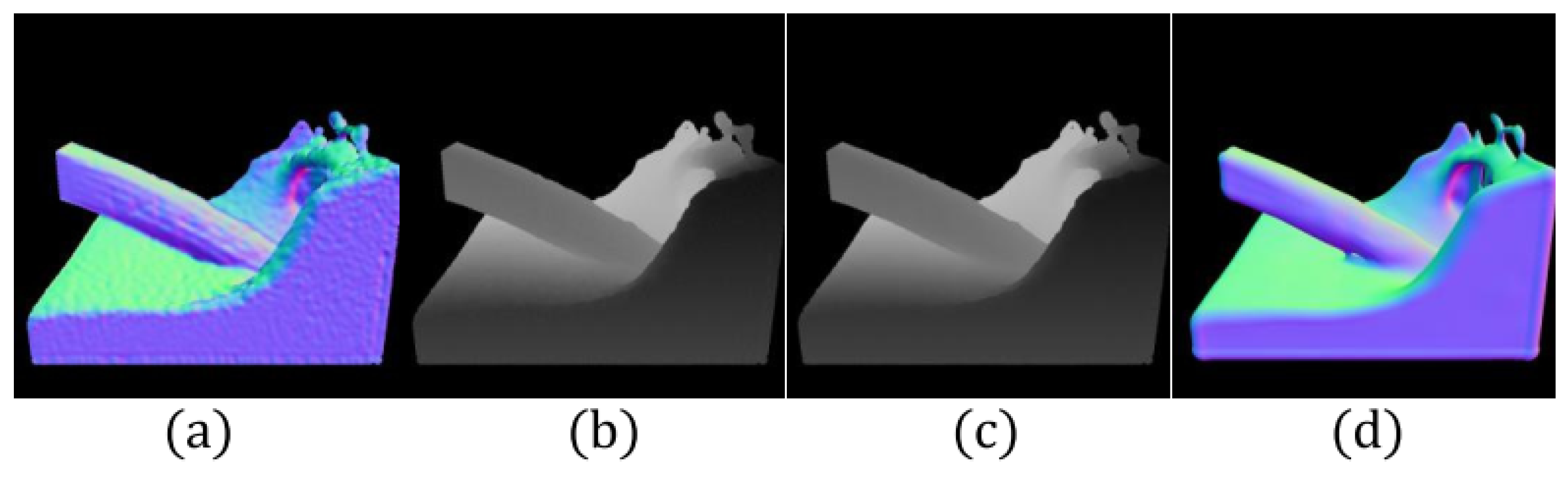
5.2. Normal Constraint Loss

We conducted experiments to investigate the effectiveness of normal constraint loss. We trained two models with and without normal constraint loss. After the training was completed, we gave the same input data to both generators, which yielded the results shown in Figure 11. Note that there are some noisy artifacts near the contour line in the image created by the model without normal constraint loss, whereas the image created by the model with normal constraint loss appears cleaner, and the edge features were captured better. This confirms that normal constraint loss plays an important role in creating a normal map. Figure 12 presents a graph of normal constraint loss over a full training run.

5.3. Training Scene

It is vitally important to confirm that the model does not overfit the training data. To ensure that this did not occur in our model, we trained the model with reduced training data and produced the results shown in Figure 13. The image used to validate the model was one frame from the dam-break scene. The comparison shown in Figure 13 reveals that the model trained with three types of scenes (Figure 13b) generated better results than the model trained with only one type of scene (Figure 13a). The model trained with six types of scenes (Figure 13c) generated results with clearer details. These results demonstrate that better performance can be achieved by adopting a variety of static and dynamic scene types.

We can conclude that our model, when trained with all the training scene data, will generate fewer artifacts than other approaches. This implies that learning a sufficient variety of types of scenes can produce good results across almost all forms of fluid simulation.

5.4. Discussion and Limitation

The results generated during the training process are presented in Figure 14. At the beginning of training, the generator acts as a filter that simply changes color. As the training progresses, the fluid surface is smoothened, and colors similar to the actual normal map are created. After sufficient training, the cGAN model generates a normal map similar to the target normal map when an input normal map is supplied.

The results presented in Figure 15 were generated using the screen-space method with a narrow-range filter, the screen-space method with a bilateral Gaussian filter, the marching-cube surface-reconstruction method with an anisotropic kernel, and our method. The marching-cube image resolution was 270 × 270 × 270, and an anisotropic kernel and vertex normal were used. For the screen-space method, the parameters were adjusted to enable the front and back of the particles to be distinguished. While using the trained cGAN, the normal map generated by the bilateral filter screen-space method was used as the input data, and validation data not previously learned were used. The result video can be found in the supplementary material.

As shown in Figure 16, the artifacts that are often observed with screen-space fluid rendering did not appear when our method was used. Moreover, the marching-cube surface-reconstruction method had an artifact involving aliasing owing to the limitation of spatial resolution of the marching cube. This artifact did not occur in our method because our method creates a normal map in the screen space.

One of our method’s limitations is that some artifacts remain for dynamic scenes where the particles are scattered. An example for such a failure is presented in Figure 17, where our method found it difficult to refine the scattered individual particles. An interesting aspect of our future work will be to investigate a hybrid method that can calculate the distribution of neighboring particles around each particle, render isolated particles via a conventional screen-space method, and render merged particles via our method.

In addition, there is the problem in that, after training, the models can be overly dependent on the parameter values used in the training data, such as the blur scale for the bilateral Gaussian filter. This problem can be alleviated by using training data with more varied parameters.

6. Conclusions

We have proposed a method that uses deep learning to refine the normal map for screen-space fluid rendering. Our method considers the cGAN model as a filter that takes a rapidly generated, rough normal map as its input and converts it to a refined normal map that is similar to the normal map extracted from a 3D reconstructed surface. We performed experiments to demonstrate that our deep normal map representation method can be successfully applied to an arbitrary fluid scene and can even obtain better results than the result generated by the traditional surface reconstruction method in some cases. Although we have focused on refining a normal map, the same algorithm could be applied to the depth map and to point clouds, in addition to fluid particles. As mentioned in the limitations section, we will make our method more robust by using training data with more varied parameters in the future.

References

1. Van der Laan, W.J.; Green, S.; Sainz, M. Screen space fluid rendering with curvature flow. In Proceedings of the 2009 Symposium on Interactive 3D Graphics and Games, Boston, MA, USA, 27 February–1 March 2009; ACM: New York, NY, USA, 2009; pp. 91–98. [Google Scholar]
2. Truong, N.; Yuksel, C. A Narrow-Range Filter for Screen-Space Fluid Rendering. Proc. ACM Comput. Graph. Interact. Tech. 2018, 1, 17. [Google Scholar] [CrossRef]
3. Radford, A.; Metz, L.; Chintala, S. Unsupervised representation learning with deep convolutional generative adversarial networks. arXiv 2015, arXiv:1511.06434. [Google Scholar]
4. Isola, P.; Zhu, J.Y.; Zhou, T.; Efros, A.A. Image-to-image translation with conditional adversarial networks. In Proceedings of the IEEE Conference on Computer Vision and Pattern Recognition, Honolulu, HI, USA, 21–26 July 2017; pp. 1125–1134. [Google Scholar]
5. Mirza, M.; Osindero, S. Conditional generative adversarial nets. arXiv 2014, arXiv:1411.1784. [Google Scholar]
6. Goodfellow, I.; Pouget-Abadie, J.; Mirza, M.; Xu, B.; Warde-Farley, D.; Ozair, S.; Courville, A.; Bengio, Y. Generative adversarial nets. In Advances in Neural Information Processing Systems; MIT Press: Cambridge, MA, USA, 2014; pp. 2672–2680. [Google Scholar]
7. Lorensen, W.E.; Cline, H.E. Marching cubes: A high resolution 3D surface construction algorithm. ACM Siggraph Comput. Graph. 1987, 21, 163–169. [Google Scholar] [CrossRef]
8. Yu, J.; Turk, G. Reconstructing surfaces of particle-based fluids using anisotropic kernels. ACM Trans. Graph. TOG 2013, 32, 5. [Google Scholar] [CrossRef]
9. Zwicker, M.; Pfister, H.; Van Baar, J.; Gross, M. Surface splatting. In Proceedings of the 28th Annual Conference on Computer Graphics and Interactive Techniques; ACM: New York, NY, USA, 2001; pp. 371–378. [Google Scholar]
10. Aurich, V.; Weule, J. Non-linear Gaussian filters performing edge preserving diffusion. In Mustererkennung 1995; Springer: Berlin/Heidelberg, Germany, 1995; pp. 538–545. [Google Scholar]
11. Müller, M.; Schirm, S.; Duthaler, S. Screen space meshes. In Proceedings of the 2007 ACM SIGGRAPH/Eurographics Symposium on Computer Animation, San Diego, CA, USA, 2–4 August 2007; Eurographics Association: Geneva, Switzerland, 2007; pp. 9–15. [Google Scholar]
12. Xiao, X.; Zhang, S.; Yang, X. Real-time high-quality surface rendering for large scale particle-based fluids. In Proceedings of the 21st ACM Siggraph Symposium on Interactive 3D Graphics and Games, San Francisco, CA, USA, 25–27 February 2017; ACM: New York, NY, USA, 2017; p. 12. [Google Scholar]
13. Burkus, V.; Kárpáti, A.; Szécsi, L. Particle-Based Fluid Surface Rendering with Neural Networks; Union: Charlotte, NC, USA, 2021. [Google Scholar]
14. Krizhevsky, A.; Sutskever, I.; Hinton, G.E. Imagenet classification with deep convolutional neural networks. In Proceedings of the Advances in Neural Information Processing Systems, Lake Tahoe, NV, USA, 3–6 December 2012; pp. 1097–1105. [Google Scholar]
15. Cho, K.; Van Merriënboer, B.; Gulcehre, C.; Bahdanau, D.; Bougares, F.; Schwenk, H.; Bengio, Y. Learning phrase representations using RNN encoder-decoder for statistical machine translation. arXiv 2014, arXiv:1406.1078. [Google Scholar]
16. Simonyan, K.; Zisserman, A. Very deep convolutional networks for large-scale image recognition. arXiv 2014, arXiv:1409.1556. [Google Scholar]
17. Ronneberger, O.; Fischer, P.; Brox, T. U-net: Convolutional networks for biomedical image segmentation. In International Conference on Medical Image Computing and Computer-Assisted Intervention; Springer: Berlin/Heidelberg, Germany, 2015; pp. 234–241. [Google Scholar]
18. Chaitanya, C.R.A.; Kaplanyan, A.S.; Schied, C.; Salvi, M.; Lefohn, A.; Nowrouzezahrai, D.; Aila, T. Interactive reconstruction of Monte Carlo image sequences using a recurrent denoising autoencoder. ACM Trans. Graph. TOG 2017, 36, 98. [Google Scholar] [CrossRef]
19. Nalbach, O.; Arabadzhiyska, E.; Mehta, D.; Seidel, H.P.; Ritschel, T. Deep shading: Convolutional neural networks for screen space shading. In Computer Graphics Forum; Wiley Online Library: Hoboken, NJ, USA, 2017; Volume 36, pp. 65–78. [Google Scholar]
20. Sanchez-Gonzalez, A.; Godwin, J.; Pfaff, T.; Ying, R.; Leskovec, J.; Battaglia, P. Learning to simulate complex physics with graph networks. In Proceedings of the International Conference on Machine Learning, Virtual Event, 12–18 July 2020; PMLR: Long Beach, CA, USA, 2020; pp. 8459–8468. [Google Scholar]
21. Shlomi, J.; Battaglia, P.; Vlimant, J.R. Graph neural networks in particle physics. Mach. Learn. Sci. Technol. 2020, 2, 021001. [Google Scholar] [CrossRef]
22. Pfaff, T.; Fortunato, M.; Sanchez-Gonzalez, A.; Battaglia, P.W. Learning mesh-based simulation with graph networks. arXiv 2020, arXiv:2010.03409. [Google Scholar]
23. Kochkov, D.; Smith, J.A.; Alieva, A.; Wang, Q.; Brenner, M.P.; Hoyer, S. Machine learning–accelerated computational fluid dynamics. Proc. Natl. Acad. Sci. USA 2021, 118, e2101784118. [Google Scholar] [CrossRef] [PubMed]
24. Dosovitskiy, A.; Brox, T. Generating images with perceptual similarity metrics based on deep networks. In Proceedings of the Advances in Neural Information Processing Systems, Barcelona, Spain, 4–9 December 2016; pp. 658–666. [Google Scholar]
25. Zhu, J.Y.; Park, T.; Isola, P.; Efros, A.A. Unpaired image-to-image translation using cycle-consistent adversarial networks. In Proceedings of the IEEE International Conference on Computer Vision, Venice, Italy, 22–29 October 2017; pp. 2223–2232. [Google Scholar]
26. Ledig, C.; Theis, L.; Huszár, F.; Caballero, J.; Cunningham, A.; Acosta, A.; Aitken, A.; Tejani, A.; Totz, J.; Wang, Z.; et al. Photo-realistic single image super-resolution using a generative adversarial network. In Proceedings of the IEEE Conference on Computer Vision and Pattern Recognition, Honolulu, HI, USA, 21–26 July 2017; pp. 4681–4690. [Google Scholar]
27. Xie, Y.; Franz, E.; Chu, M.; Thuerey, N. tempogan: A temporally coherent, volumetric gan for super-resolution fluid flow. ACM Trans. Graph. TOG 2018, 37, 95. [Google Scholar] [CrossRef]
28. Wang, T.C.; Liu, M.Y.; Zhu, J.Y.; Liu, G.; Tao, A.; Kautz, J.; Catanzaro, B. Video-to-Video Synthesis. In Proceedings of the Advances in Neural Information Processing Systems (NeurIPS), Montreal, QC, Canada, 3–8 December 2018. [Google Scholar]
29. Pathak, D.; Krahenbuhl, P.; Donahue, J.; Darrell, T.; Efros, A.A. Context encoders: Feature learning by inpainting. In Proceedings of the IEEE Conference on Computer Vision and Pattern Recognition, Las Vegas, NV, USA, 27–30 June 2016; pp. 2536–2544. [Google Scholar]
30. Zhao, H.; Gallo, O.; Frosio, I.; Kautz, J. Loss functions for image restoration with neural networks. IEEE Trans. Comput. Imaging 2016, 3, 47–57. [Google Scholar] [CrossRef]
31. Müller, M.; Charypar, D.; Gross, M. Particle-based fluid simulation for interactive applications. In Proceedings of the 2003 ACM SIGGRAPH/Eurographics Symposium on Computer Animation, San Diego, CA, USA, 26–27 July 2003; Eurographics Association: Geneva, Switzerland, 2003; pp. 154–159. [Google Scholar]
32. Macklin, M.; Müller, M. Position based fluids. ACM Trans. Graph. TOG 2013, 32, 104. [Google Scholar] [CrossRef]
33. Maas, A.L.; Hannun, A.Y.; Ng, A.Y. Rectifier nonlinearities improve neural network acoustic models. Proc. ICML 2013, 30, 3. [Google Scholar]
34. He, K.; Zhang, X.; Ren, S.; Sun, J. Deep residual learning for image recognition. In Proceedings of the IEEE Conference on Computer Vision and Pattern Recognition, Las Vegas, NV, USA, 27–30 June 2016; pp. 770–778. [Google Scholar]
35. Kingma, D.P.; Ba, J. Adam: A method for stochastic optimization. arXiv 2014, arXiv:1412.6980. [Google Scholar]
36. Abadi, M.; Barham, P.; Chen, J.; Chen, Z.; Davis, A.; Dean, J.; Devin, M.; Ghemawat, S.; Irving, G.; Isard, M.; et al. Tensorflow: A system for large-scale machine learning. In Proceedings of the 12th {USENIX} Symposium on Operating Systems Design and Implementation ({OSDI} 16), Savannah, GA, USA, 2–4 November 2016; pp. 265–283. [Google Scholar]
37. Thomas, M.M.; Forbes, A.G. Deep Illumination: Approximating Dynamic Global Illumination with Generative Adversarial Network. arXiv 2017, arXiv:1710.09834. [Google Scholar]
Figure 1. (a) Rendering via a bilateral Gaussian filter [1]. (b) Rendering via our approach.
Applsci 11 09065 g001
Figure 2. Algorithm overview: (a) the training part and (b) the rendering part.
Applsci 11 09065 g002
Figure 3. Normal constraint loss comparison: (a) the input normal map, (b) the target normal map, (c) the generated normal map without normal constraint loss, and (d) the generated normal map with normal constraint loss.
Applsci 11 09065 g003
Figure 4. Loss comparison: (a) the input normal map, (b) the target normal map, (c) the generated normal map using the L2 loss function, and (d) the generated normal map using the L1 loss function.
Applsci 11 09065 g004
Figure 5. Examples of the training data: (a) the normal map generated by the screen-space rendering method, (b) the depth map, (c) the blurred depth map, and (d) the normal map generated by the surface-reconstruction method.
Applsci 11 09065 g005
Figure 6. Various types of scenes.
Applsci 11 09065 g006
Figure 7. (a) 1024 × 1024 image, (b) 512 × 512 upsampled image cropped from a 1024 × 1024 image.
Applsci 11 09065 g007
Figure 8. Model architecture: (left) the model’s generator architecture and (right) the discriminator architecture. y is the conditional data, z is the noise data, x ˜ is the generated data, and x is the target data.
Applsci 11 09065 g008
Figure 9. Comparisons of the results obtained with and without the auxiliary features.
Applsci 11 09065 g009
Figure 10. (a) When an edge is generated on a similar normal distribution case, and (b) when an edge is generated in a non-similar normal distribution.
Applsci 11 09065 g010
Figure 11. Comparison of the results obtained by the models with and without the normal constraint loss.
Applsci 11 09065 g011
Figure 12. Convergence of the normal constraint loss.
Applsci 11 09065 g012
Figure 13. Comparison of the generated normal map results for (a) training with one scene (Sphere Crown), (b) training with three scenes (Merging Fluid, Pouring Fluid, and Double Pouring Fluid), and (c) training with all scenes. The various scene types are shown in Figure 6.
Applsci 11 09065 g013
Figure 14. Left to right, the columns present input, target, and our result. (a) epoch 0 (b) epoch 5 (c) epoch 10.
Applsci 11 09065 g014
Figure 15. Comparison of the rendering results.
Applsci 11 09065 g015
Figure 16. Close-ups of the rendering results for obtained using our method, the screen-space (bilateral Gaussian filter) method, and the surface reconstruction method.
Applsci 11 09065 g016
Figure 17. Failure case: (a) the input image, (b) the target image, and (c) the result obtained by our method.
Applsci 11 09065 g017
Publisher’s Note: MDPI stays neutral with regard to jurisdictional claims in published maps and institutional affiliations.