Study on Wind Field Characteristics in a Coastal Plain Based on a New Three-Dimensional Joint Distribution Model

Abstract

This paper studied the joint probability distribution of wind speed, wind direction, and wind height. The measured wind field data of a coastal plain in Zhongshan city, Guangdong Province, China, were taken as the research object. A three-dimensional joint distribution modeling method, based on the copula function and the AL (angular–linear) model, is proposed. Firstly, the wind speed is modeled by the common distribution model, and the Weibull distribution is selected. Secondly, the mvM (mixed von Mises distribution) was used to fit the wind direction probability density, and the joint distribution of wind speed and wind direction was established based on the AL model. Finally, a three-dimensional joint distribution model of wind speed, wind direction, and height was established by considering the effect of height through the copula function. The results showed that Weibull distribution can better describe the wind speed distribution in this region. The north–south wind prevailed in this region, and the probability of the main wind direction decreased with the increase in height. The joint distribution of wind speed and direction, based on the AL model, fitted well with the measured data, and the final three-dimensional distribution model had a good fitting effect.

1. Introduction

As a common natural phenomenon, wind profoundly affects our lives. On the one hand, with the development of society and the global economy, humankind’s demand for energy is increasing, and wind energy has been widely used as a clean energy in recent years [1,2]. On the other hand, the volume of human buildings is gradually increasing, and more and more skyscrapers and large-span bridges have appeared, which are particularly sensitive to wind [3]. Whether it is for wind energy evaluation or structural wind resistance design, the study of wind characteristics is of fundamental importance. The most direct and effective way of studying wind characteristics is to measure them. For huge measured data, using the appropriate distribution model of wind speed and direction can simply and effectively describe its law. Many scholars have carried out extensive research on this.

Christopher Jung et al. [4] evaluated 115 different wind speed distribution models, as proposed in 46 articles from 2010 to 2018, according to the quantity and quality of analysis data; the results showed that five-parameter Wakeby distribution and four-parameter Kappa distribution scored the highest. Ilhan Usta et al. [5] proposed an innovative method, PWMBP (probability weighted moments based on the power density method), which was developed and proposed for estimating the Weibull parameters in wind energy applications. Jianzhou Wang et al. [6] took four locations in central China as examples to compare commonly used wind speed probability distribution models and estimation methods of corresponding parameters. The results showed that the nonparametric model had better fitting accuracy and operation simplicity, and that the random heuristic algorithm was better than the widely used estimation method. Christopher Jung et al. [7] compared the goodness of fit between 24 single-component probability density functions, 21 mixed probability density functions, and empirical wind speed probability density functions worldwide. They found that the five-parameter Wakeby probability density function was suitable for land wind speed and the four-parameter Kappa probability density function was suitable for sea wind speed. The two-parameter Weibull probability density function is only optimal for a few wind speeds. Fatma Gul Akgul et al. [8] used the inverse Weibull (IW) distribution to model wind speed, and the results showed that, in most cases, IW distribution based on ML and MML parameter estimation had better results than Weibull distribution, based on corresponding estimation. Talha Arslan et al. [9] used generalized Lindley (GL) distribution and power Lindley (PL) distribution to model wind speed data. The results show that both GL distribution and PL distribution can provide the best fit according to different evaluation criteria.

Many scholars have carried out research on the distribution of wind speed, but in many cases, wind direction also needs to be focused on; therefore, some scholars have conducted research on the distribution of wind direction and the joint distribution of wind direction and speed, through which the influence of wind direction can be considered. Jose A. Carta et al. [10] used von Mises (vM-pdf) finite mixed distribution to represent the distribution of directional wind speed. Analysis of wind direction data from several weather stations in the Canary Islands shows that the model is suitable for wind conditions in areas with multiple patterns of prevailing wind directions. Wang Hao et al. [11] predicted the basic wind speed of Sutong Bridge based on the joint distribution of wind speed and direction. X.W. Ye et al. [12] proposed extended parameter estimation algorithms for multivariate and multi-peak cyclic distribution to build a joint distribution model of wind speed and direction. It was found that the model had good representativeness, and that the algorithm could save significant amounts of time in parameter estimation. Qinkai Han et al. [13] proposed the use of non-parametric kernel density (NP-KD) and non-parametric JW (NP-JW) models. It was shown that the non-parametric models (NP-KD, NP-JW) generally outperformed the parametric models (AG, Weibull, Rayleigh, JW-TNW, JW-FMN) and showed a more robust performance in fitting the joint speed and direction distributions. Zheng Xiaowei et al. [14] used the multiplication theorem and the AL model to model the joint probability distribution of wind speed and direction, respectively. The results show that the joint probability density function of wind speed and direction derived from the AL model is better than that based on the multiplication theorem, and that ignoring the effects of wind direction significantly improves estimates of extreme wind speeds. Dong Sheng et al. [15,16] proposed a new method for establishing a joint distribution model, based on a wind rose diagram using a continuous AL joint distribution model, drawing a new wind speed and direction distribution diagram. The results show that the statistical model has high reliability and a strong correlation with the original data distribution.

Previous researchers have mainly focused on the modeling of wind speed distribution or joint distribution of wind speed and direction, i.e., one or two-dimensional joint distribution models; however, for wind power in small geographic areas, in areas with complex tall buildings [17,18] and so on, it is necessary to take three-dimensional joint distribution into consideration. Specifically, the spatial correlation of wind power is concerned when clusters of wind generators are spread over small geographic areas, and a suitable three-dimensional joint distribution model can describe the correlation suitably. For flexible tall buildings, wind-induced dynamic responses are three-dimensional, so the three-dimensional wind load should be clearly described. For the third dimension, the height direction, the change in wind speed is usually considered by exponential law and logarithmic law; however, some studies [19,20] show that these laws do not describe the variation law of wind speed in some areas. Therefore, the three-dimensional modeling of wind speed probability distribution is necessary. Based on the AL (angular–linear) model and the copula function, this paper proposes a modeling method to describe the three-dimensional distribution of wind speed.

2. Materials and Methods

2.1. Copula Function

In 1959, Sklar [21] proposed that an n-dimensional joint distribution function could be decomposed into n edge distribution functions and a copula function, which describes the correlation between variables. Nelson [22] provided a strict definition of the copula function in 1999. The copula function is a connecting function that connects the joint distribution function $F(x_1,x_2,\cdots x_N)$ of random variables $X_1,X_2,\cdots X_N$ with their respective edge distribution functions $F_{X_1}(x_1),F_{X_2}(x_2),\cdots F_{X_N}(x_N)$, that is, function $C({\mu }_1,{\mu }_2,\cdots {\mu }_N)$,

$$F(x_1,x_2,\cdots x_N)=C[F_{X_1}(x_1),F_{X_2}(x_2),\cdots F_{X_N}(x_N)]$$

(1)

When the edge distribution of each random variable is known, it is easy to calculate their joint distribution function using the copula function. At present, the copula function is mainly used in financial fields [23,24,25], for measurements such as that of value-at-risk of multiple financial assets.

Table 1 lists some commonly used copula functions.

Table 1. Commonly used copula functions.

Function	Expression	Parameter	Clan
Gumbel-	$\exp \left(-{\left[{\displaystyle \sum _{i=1}^N{(-\ln u_i)}^{\theta }}\right]}^{1/\theta }\right)$	$\theta \in [1,+\infty )$	Archimedes/Extremum
Frank-	$\frac{1}{\theta }\ln \left(1+(\underset{i=1}{\overset{N}{\mathrm{\Pi }}}(\exp (-\theta u_i)-1))/{(\exp (-\theta )-1)}^{N-1}\right)$	$\theta \in (-\infty ,+\infty )$	Archimedes
Clayton-	${\left({\displaystyle \sum _{i=1}^N{u}_i{}^{-\theta }-N+1}\right)}^{-1/\theta }$	$\theta \in (0,+\infty )$	Archimedes
Gaussian-	${\mathrm{\Phi }}_{\theta }({\mathrm{\Phi }}^{-1}(u_1),{\mathrm{\Phi }}^{-1}(u_2),\cdots {\mathrm{\Phi }}^{-1}(u_N))$	$\theta \in (-1,1)$	Ellipse
Student’s t-	$T_{\theta ,\lambda }(T_{\lambda }^{-1}(u_1),T_{\lambda }^{-1}(u_2),\cdots T_{\lambda }^{-1}(u_N))$	$\theta \in (-1,1),\lambda \in (0,+\infty )$	Ellipse

2.2. AL–Copula Three-Dimensional Wind Speed Probability Distribution Model

Johnson and Wehrly [26] derived the angular–linear distribution model from the maximum entropy principle, and used it to describe the joint probability distribution of wind speed and direction. The joint probability density function is

$$f(v,\theta )=2\pi g(\zeta )f(v)f(\theta )$$

(2)

Among them, $f(v)$ is the wind speed probability density function of the full wind direction, which can be described by commonly used wind speed probability distribution models. $f(\theta )$ is the wind direction angle probability density function, which can be described by the mixed von Mises distribution (mvM) [10]. Its probability density function is

$$f(\theta )={\displaystyle \sum _i^N{\omega }_i}\frac{\exp [k_i\cos (\theta -{\mu }_i)]}{2\pi I_0(k_i)}$$

(3)

In Equations:

$$\begin{array}{l}\theta :wind \mathrm{angle},0\le \theta <2\pi \\ {\mu }_i:average \mathrm{wind} \mathrm{direction},0\le {\mu }_i<2\pi \\ {\omega }_i:weight,0\le {\omega }_i<1,{\displaystyle \sum {\omega }_i}=1\\ k_i:\mathrm{scale} \mathrm{parameters},k_i\ge 0\\ I_0(k_i):\mathrm{zero}\text{-}\mathrm{order} \mathrm{modified} \mathrm{type} \mathrm{{\rm I}} Bessel \mathrm{equation}\end{array}$$

$g(\zeta )$ is the probability density function of parameter ζ, which is obtained by fitting the mvM. Among them

$$\zeta =\{\begin{array}{c}2\pi [F(v_i)-F({\theta }_i)] , F(v_i)\ge F({\theta }_i)\\ 2\pi +2\pi [F(v_i)-F({\theta }_i)] , F(v_i)<F({\theta }_i)\end{array}$$

(4)

When fitting the high order mixed von Mises distribution, giving a better initial value of parameters can significantly improve the accuracy and efficiency of the fitting. Carta [10] proposed a calculation method to determine the initial value of parameters in the mvM. Firstly, the wind direction data are divided into the following N groups: $0^{\circ }-{\theta }_1,{\theta }_1-{\theta }_2,\cdots {\theta }_{i-1}-{\theta }_i,{\theta }_{N-1}-{\theta }_N({\theta }_N={360}^{\circ })$. Among them, the number of samples in the i-th group $[{\theta }_{i-1}-{\theta }_i)$ is $n_i$. The initial value can be calculated using the following formula:

$${\omega }_i=\frac{n_i}{{\displaystyle \sum _{i=1}^N{n}_i}}$$

(5)

$${\mu }_i=\{\begin{array}{cc}\arctan (\frac{s_i}{c_i})& ,s_i\ge 0,c_i>0\\ \frac{\pi }{2}& ,s_i>0,c_i=0\\ \pi +\arctan (\frac{s_i}{c_i})& ,c_i<0\\ 2\pi +\arctan (\frac{s_i}{c_i})& ,s_i<0,c_i>0\\ \frac{3\pi }{2}& ,s_i<0,c_i=0\end{array}$$

(6)

$k_i$ can be obtained by the following formula:

$$\frac{I_1(k_i)}{I_0(k_i)}={(s_i^2+c_i^2)}^{0.5}$$

(7)

$$s_i=\frac{{\displaystyle \sum _{j=1}^{n_i}\sin {\theta }_j}}{n_i},c_i=\frac{{\displaystyle \sum _{j=1}^{n_i}\cos {\theta }_j}}{n_i}$$

(8)

The previous copula function is used to connect the distribution of one-dimensional random variables. This paper attempts to connect the joint distribution of two-dimensional random variables with the copula function. Firstly, the AL model is used to describe the joint distribution of wind speed and direction at each height $F_{V_1{\theta }_1}(v_1,{\theta }_1),F_{V_2{\theta }_2}(v_2,{\theta }_2),\cdots F_{V_N{\theta }_N}(v_N,{\theta }_N)$. Then, the joint distribution of wind speed and wind direction at each height is connected by the copula function to construct the three-dimensional joint distribution of wind speed, wind direction, and height. The expression of the AL–Copula three-dimensional wind speed probability distribution model is as follows:

$$F(x_1,x_2,\cdots x_N)=C[F_{V_1{\theta }_1}(v_1,{\theta }_1),F_{V_2{\theta }_2}(v_2,{\theta }_2),\cdots F_{V_N{\theta }_N}(v_N,{\theta }_N)]$$

(9)

3. Results

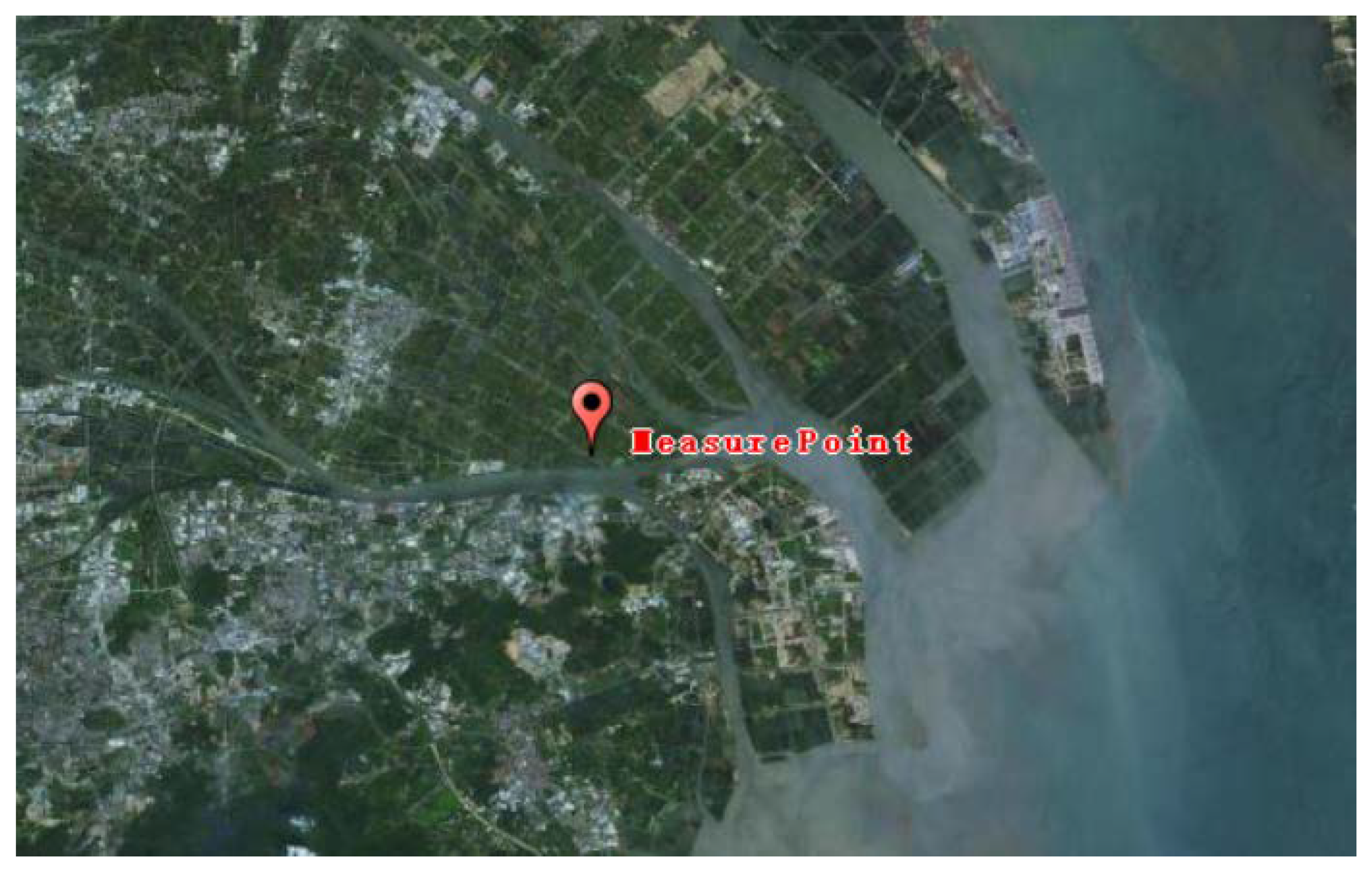
The sample of this calculation example came from the measured data. The observation instrument was a VT-1 phased array Doppler radar system. The wind observation location was near the Hengmen Waterway, which is a typical coastal plain area. The Hengmen Waterway is in the east of Zhongshan City, Guangdong Province, China. It starts at Dananwei, Gangkou Town (the junction of the Jiya Waterway and Xiaolan Waterway) and enters the sea at Hengmen Mountain. As shown in Figure 1, the surrounding area of the observation site is dominated by fish ponds, the terrain is flat, the water surface is open, and there are few obstructions. The height of the sample was 30 m–180 m. The observation time was the whole year of 2020. After screening, the number of valid samples for the study was 8270.

Figure 1. Location of measuring point.

3.1. Probability Density Function of All Wind Speeds

To keep the model as simple as possible, this paper compares the fitting effects of three common distribution models. The functional expressions of the three distribution models are shown in Table 2.

Table 2. Common wind speed probability distribution model.

Distribution Model	Weibull Distribution	Gamma Distribution	Lognormal Distribution
Probability Density Function	$f(v)=\frac{k}{c}{(\frac{v}{c})}^{k-1}{e}^{-{(\frac{v}{c})}^k}$	$f(v)=\frac{v^{k-2}}{c^k\mathrm{\Gamma }(k)}{e}^{-(\frac{v}{c})}$	$f(v)=\frac{v^{k-2}}{v{\sigma }_0\sqrt{2\pi }}e\frac{-{(\ln v-{\mu }_0)}^2}{2{\sigma }_0}$
Cumulative Distribution Function	$F(v)=1-e^{-{(\frac{v}{c})}^k}$	$F(v)=\frac{\mathrm{\Gamma }\frac{v}{c}(k)}{\mathrm{\Gamma }(k)}$	$F(v)=\mathrm{\Phi }(\frac{\ln v-{\mu }_0}{{\sigma }_0})$
Estimated parameters	Scale parameter c, Shape parameter k	Scale parameter c, Shape parameter k	Position parameter μ0, Scale parameter σ0

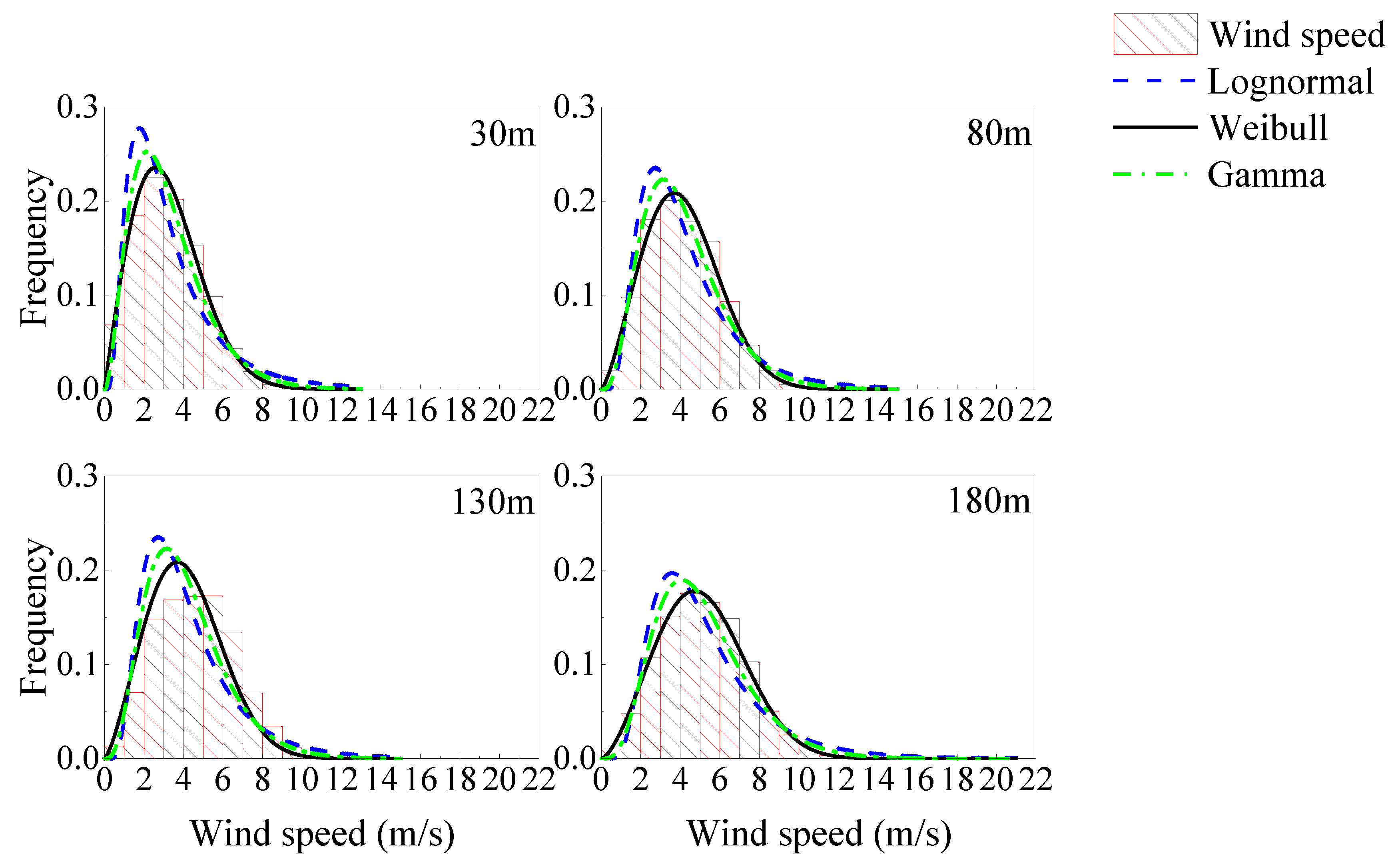
Figure 2 shows the fitting effect of different probability distribution models on wind speed distribution at each height. The A–D method is used to test the goodness of fit of each distribution model. It can be seen in the figure that the probability of high wind speed increases with increased height; however, overall, the wind speed is mainly concentrated in low wind speed. As shown in Table 3, this group of samples better obeys the Weibull distribution. Therefore, the subsequent work will use the Weibull distribution to describe wind speed distribution; the Weibull distribution parameters at each height are shown in Table 4.

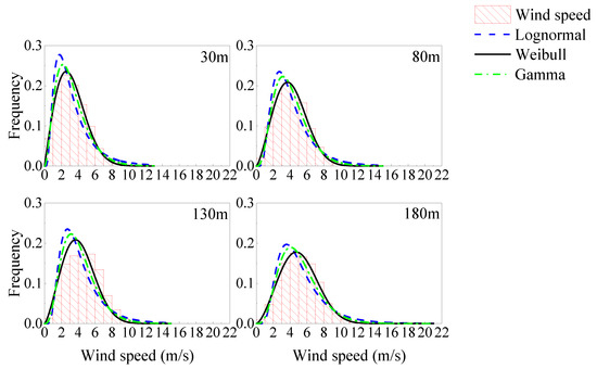
Figure 2. Wind speed probability distribution.

Table 3. Goodness-of-fit test of distribution model.

Height (m)	Goodness-of-Fit Test (A–D Test)
	Lognormal Distribution	Weibull Distribution	Gamma Distribution
30	117.67859	3.12768	29.16908
40	101.15522	3.77735	20.73015
50	86.83476	11.36016	21.57331
60	83.15549	5.2625	22.8545
70	84.38502	4.56088	24.49062
80	88.26657	3.90411	25.50058
90	84.07432	3.72759	22.2613
100	90.78233	4.77145	27.25642
110	93.99505	7.09786	32.82279
120	102.19729	5.5742	38.62026
130	108.79653	5.66863	41.60047
140	105.66157	4.06106	39.41389
150	106.74012	3.00408	38.5011
160	96.69295	2.45435	33.79262
170	104.77383	2.79012	36.42134
180	107.23918	2.47474	35.762

Table 4. Parameters of the Weibull distribution model at different heights.

Height (m)	α	β
30	3.64485	2.00181
40	3.39006	1.80455
50	3.55701	1.7978
60	4.3308	2.28137
70	4.57121	2.37895
80	4.64485	2.37083
90	4.56443	2.27996
100	4.70691	2.30711
110	4.87823	2.36004
120	5.14665	2.51522
130	5.19367	2.48331
140	5.36856	2.57419
150	5.47269	2.59135
160	5.58688	2.60495
170	5.65285	2.56085
180	5.75441	2.54396

3.2. Wind Speed–Direction Joint Distribution

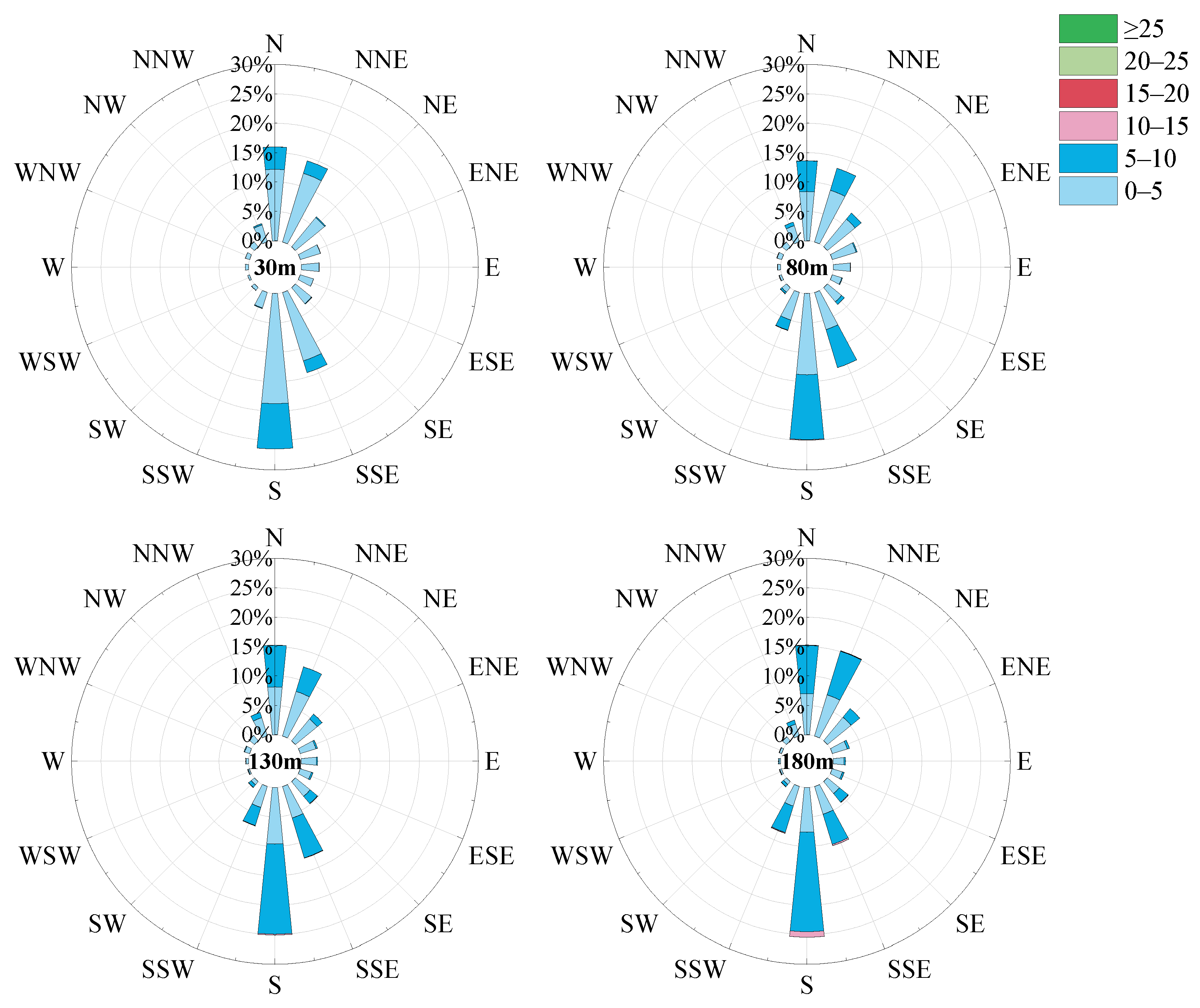
In Figure 3, the distribution of wind speed in different wind directions can be seen intuitively. The wind directions in this area are mainly in the north and south directions, which are consistent with the climate characteristics of the southern coastal areas of China. This paper uses the AL model to describe the joint distribution of wind speed and wind direction.

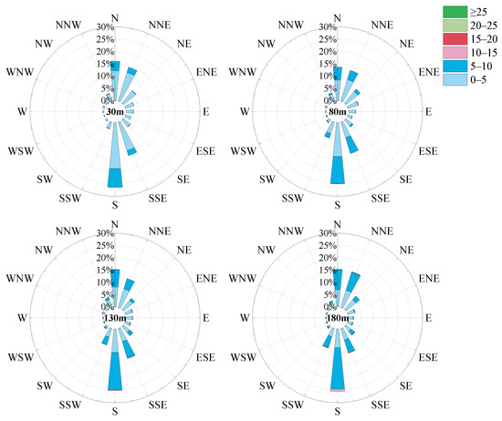
Figure 3. Wind rose at different heights.

Research shows [10] that the sixth-order mvM can describe the wind direction distribution well, and that the low-order mvM can fit $g(\zeta )$ well. This paper calculated the fitting parameters of the mvM from the second to the seventh order for the wind direction distribution. Due to space limitations, this article only gives the fitting results of different orders of the 30 m height, as shown in Table 5.

Table 5. Results and effects of each order fitting parameter at 30 m height.

	Order	7	6	5	4	3	2
Parameter
k1		15.1200	13.8300	13.7100	13.8200	11.5800	7.6120
k2		3.4140	1.1610	1.1200	1.3100	0.8083	23.6900
k3		46.6900	592.4000	68.8500	68.3600	30.2400
k4		46.9200	59.1600	12.4800	12.0200
k5		330.8000	10.5900	61.2100
k6		0.7352	61.5400
k7		79.3300
u1		0.1984	0.2273	0.2282	0.1756	0.1915	0.2260
u2		0.4825	0.8841	0.9113	0.9020	1.6960	3.0250
u3		2.7010	2.7150	3.0650	3.0640	3.0340
u4		3.0570	3.0590	2.9520	2.9510
u5		3.4110	2.9440	6.2830
u6		1.9110	6.2830
u7		6.2800
w1		0.2265	0.2491	0.2512	0.2875	0.3346	0.4284
w2		0.1400	0.2710	0.2726	0.2649	0.2952	0.4366
w3		0.0730	0.0077	0.1691	0.1713	0.3776
w4		0.3204	0.2076	0.2704	0.2743
w5		0.0104	0.2280	0.0378
w6		0.2066	0.0376
w7		0.0261
R2		0.9787	0.9786	0.9780	0.9763	0.9619	0.9203

Considering the simplicity of the model as much as possible, while taking into account the overall goodness of fit of the three-dimensional distribution model, this study finally adopted the fifth-order mvM. The wind direction probability density function parameters at each height are shown in Table 6. It can be seen that the fifth-order mvM model has a good fitting effect on wind direction distribution, with an R² parameter as high as 0.92 or more.

Table 6. Parameter fitting value of $f(\theta )$.

Height(m)	k1	k2	k3	k4	k5	u1	u2	u3	u4	u5	w1	w2	w3	w4	w5	R2
30	13.7100	1.1200	68.8500	12.4800	61.2100	0.2282	0.9113	3.0650	2.9520	6.2830	0.2512	0.2726	0.1691	0.2704	0.0378	0.9780
40	52.8300	12.1300	20.8500	64.9700	0.5033	0.0832	0.1685	3.0270	3.1170	1.1230	0.0847	0.2782	0.1969	0.2129	0.2312	0.9766
50	66.6700	18.4000	19.9600	114.0000	0.8051	0.0560	0.2575	3.0450	3.1150	1.1330	0.0832	0.2039	0.2176	0.2199	0.2766	0.9822
60	13.8900	321.6000	17.1600	0.8760	38.6700	0.3152	2.9980	3.0520	1.1880	6.2830	0.2020	0.0415	0.4024	0.2765	0.0793	0.9710
70	10.9200	1.4450	11.7100	395.5000	529.5000	0.2020	0.9131	3.0620	2.9720	3.1140	0.2673	0.2562	0.4069	0.0457	0.0187	0.9694
80	11.7100	11.3000	106.0000	1.1640	23.9800	0.3307	3.0720	3.0150	0.8896	6.2830	0.1770	0.3941	0.0656	0.2812	0.0836	0.9686
90	9.3340	1.0250	9.7470	79.1600	19.9200	0.3040	0.8569	3.0470	3.0100	6.2830	0.1775	0.2987	0.3707	0.0791	0.0747	0.9566
100	9.2550	2.2240	5.2980	29.6300	5.3990	0.1421	0.9106	3.0010	3.0450	5.0800	0.2592	0.2206	0.3049	0.1931	0.0259	0.9543
110	9.6020	1.0870	489.7000	29.6900	6.3710	0.1726	0.9397	2.9100	3.0950	2.9980	0.2449	0.2934	0.0130	0.1867	0.2639	0.9583
120	9.8490	0.7306	55.2100	15.9600	54.9000	0.2483	1.1830	2.4370	3.0720	6.2010	0.2427	0.2850	0.0220	0.4171	0.0365	0.9670
130	15.5900	5.4960	46.0400	17.4900	0.5679	0.0945	0.4032	2.4590	3.0890	1.5540	0.1985	0.1299	0.0314	0.4082	0.2343	0.9623
140	19.8100	13.0900	40.2700	15.3600	0.8162	0.0000	0.4384	2.4440	3.0980	0.9455	0.1299	0.1335	0.0367	0.4127	0.2897	0.9636
150	8.9870	3.1880	3.7330	20.6500	7.5860	0.1108	0.7274	2.8700	3.1300	5.1230	0.2474	0.1976	0.2615	0.2726	0.0222	0.9581
160	22.5100	33.7600	4.0460	50.7100	2.5220	3.1490	0.0000	2.8980	0.4082	0.4151	0.2493	0.0922	0.2819	0.0430	0.3304	0.9652
170	6.6820	0.6062	28.8100	15.4500	62.3500	0.2638	1.1850	2.4790	3.1390	6.2380	0.2842	0.2343	0.0548	0.3971	0.0320	0.9646
180	20.5900	2.9850	25.8800	99.9700	3.5700	0.2392	0.4578	3.1490	0.0333	2.9180	0.1665	0.2657	0.2676	0.0366	0.2627	0.9672

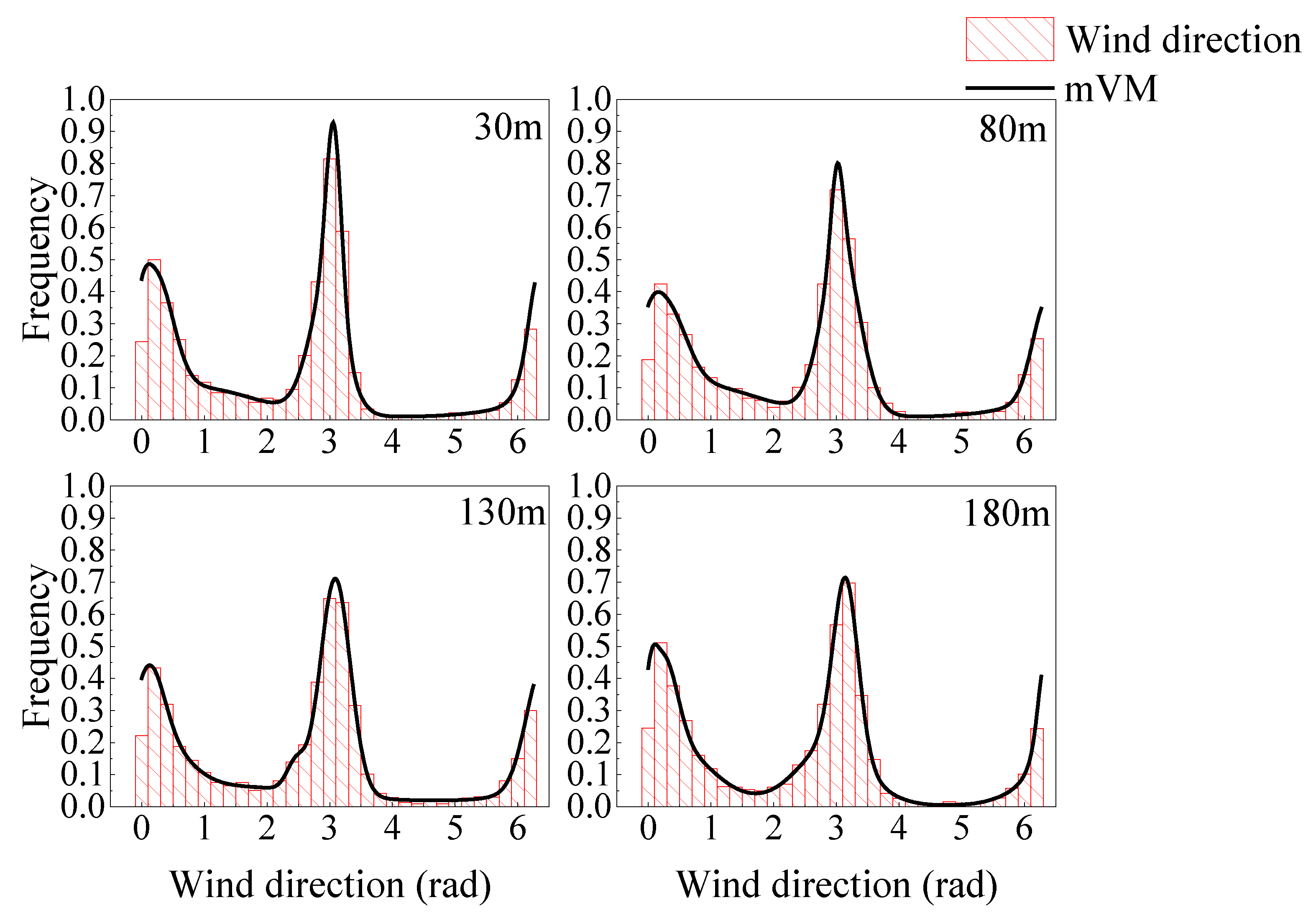
Finally, the fitting effect of the function on wind direction distribution is shown in Figure 4. Similarly, the third-order mixed distribution was used to describe the correlation coefficients of wind speed and wind direction, and the results are shown in Table 7.

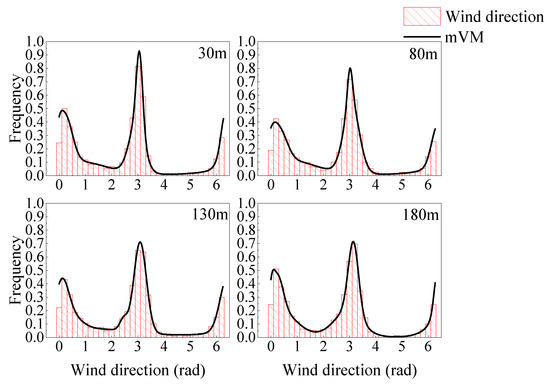
Figure 4. Results of the fitting of wind.

Table 7. Parameter fitting value of $g(\zeta )$.

Height (m)	k1	k2	k3	u1	u2	u3	w1	w2	w3	R2
30	0.6672	147.8000	1.3400	4.9220	5.6180	1.5220	0.6452	0.0135	0.3460	0.9788
40	0.5144	2.8280	4.6260	1.6050	4.5070	5.5370	0.7490	0.1400	0.1110	0.9752
50	53.3900	2.1320	0.5736	0.9577	1.6970	5.1360	0.0291	0.2269	0.7489	0.9804
60	0.6317	1.2940	13.5200	1.8460	5.1140	0.8774	0.6311	0.3480	0.0209	0.9547
70	4.0900	2.6680	0.4680	1.0640	2.2170	5.1050	0.1079	0.1783	0.7138	0.982
80	1.6190	5.3890	0.6176	1.3280	2.6010	4.9860	0.2995	0.0913	0.6092	0.9554
90	4.0300	0.3784	1.9390	2.5790	5.2240	1.3990	0.1006	0.6953	0.2041	0.9839
100	0.4858	1.7340	4.0630	5.1250	1.3430	2.6130	0.6476	0.2541	0.0984	0.9793
110	1.2830	3.5460	0.7891	1.2230	2.6220	5.0040	0.3694	0.1188	0.5119	0.9743
120	1.2510	6.5100	0.7259	1.3440	2.7020	4.9620	0.3793	0.0675	0.5532	0.9553
130	0.2516	9.0010	4.6660	1.1730	2.5760	4.8990	0.8914	0.0215	0.0871	0.9066
140	1.1460	1.6970	0.8594	5.0090	0.6983	2.3080	0.3560	0.2202	0.4238	0.9755
150	0.2522	10.7400	5.2870	1.0770	3.1060	4.8310	0.9289	0.0142	0.0569	0.9259
160	0.7875	1.8100	1.7690	0.8724	2.8150	4.8900	0.5837	0.1912	0.2252	0.9514
170	2.8060	1.7220	0.5832	2.8900	4.8850	1.0080	0.1054	0.2051	0.6895	0.9066
180	10.9900	2.4180	0.2066	2.2860	4.6390	0.6778	0.0171	0.0924	0.8906	0.959

In our calculations, we found that using the process shown in Figure 5 to determine the parameters could improve the accuracy of the mvM model:

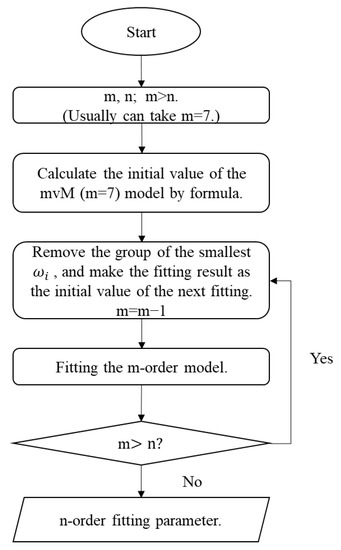
Figure 5. Flow chart of parameter determination of mvM model.

We grouped the measured samples at the measuring points and calculated the i-th wind speed interval $[v_i,v_{i+1}]$ and the j-th wind direction interval $[{\theta }_j,{\theta }_{j+1}]$ (number of samples $n_{ij}$). The joint probability density of measured wind speed and direction can be expressed as follows:

$$p_{ij}=\frac{n_{ij}}{N_{\Delta }{v}_{i\Delta }{\theta }_j}$$

(10)

In the formula, $N$ is the number of measured wind speed samples, $\Delta v_i=v_{i+1}-v_i$, $\Delta {\theta }_j={\theta }_{j+1}-{\theta }_j$.

This paper takes $\Delta v_i=1 \mathrm{m}/\mathrm{s}$, $\Delta {\theta }_j=22.5\times \pi /180 \mathrm{rad}$, divides 21 × 16 grids, and calculates the $p_{ij}$ and the probability density function $f(v_i+\Delta v_i/2,{\theta }_j+\Delta {\theta }_j/2)$ corresponding to the midpoint of the grid $(v_i+\Delta v_i/2,{\theta }_j+\Delta {\theta }_j/2)$. The coefficient of determination, R2, is used to evaluate the wind speed and wind direction joint distribution model:

$$R^2=1-\frac{{\displaystyle \sum _{i=1}^{21}{\displaystyle \sum _{j=1}^{16}{(p_{ij}-f_{ij})}^2}}}{{\displaystyle \sum _{i=1}^{21}{\displaystyle \sum _{j=1}^{16}{(p_{ij}-\overline{p_{ij}})}^2}}}$$

(11)

The results are shown in Table 8, which shows that the fitting effect of the two-dimensional joint distribution model is good.

Table 8. Goodness-of-fit test of AL model.

Height(m)	30	40	50	60	70	80	90	100
R2	0.8502	0.8536	0.8441	0.8399	0.8146	0.8582	0.8578	0.8552
Height(m)	110	120	130	140	150	160	170	180
R2	0.8399	0.8545	0.8466	0.8717	0.8721	0.8838	0.8843	0.8997

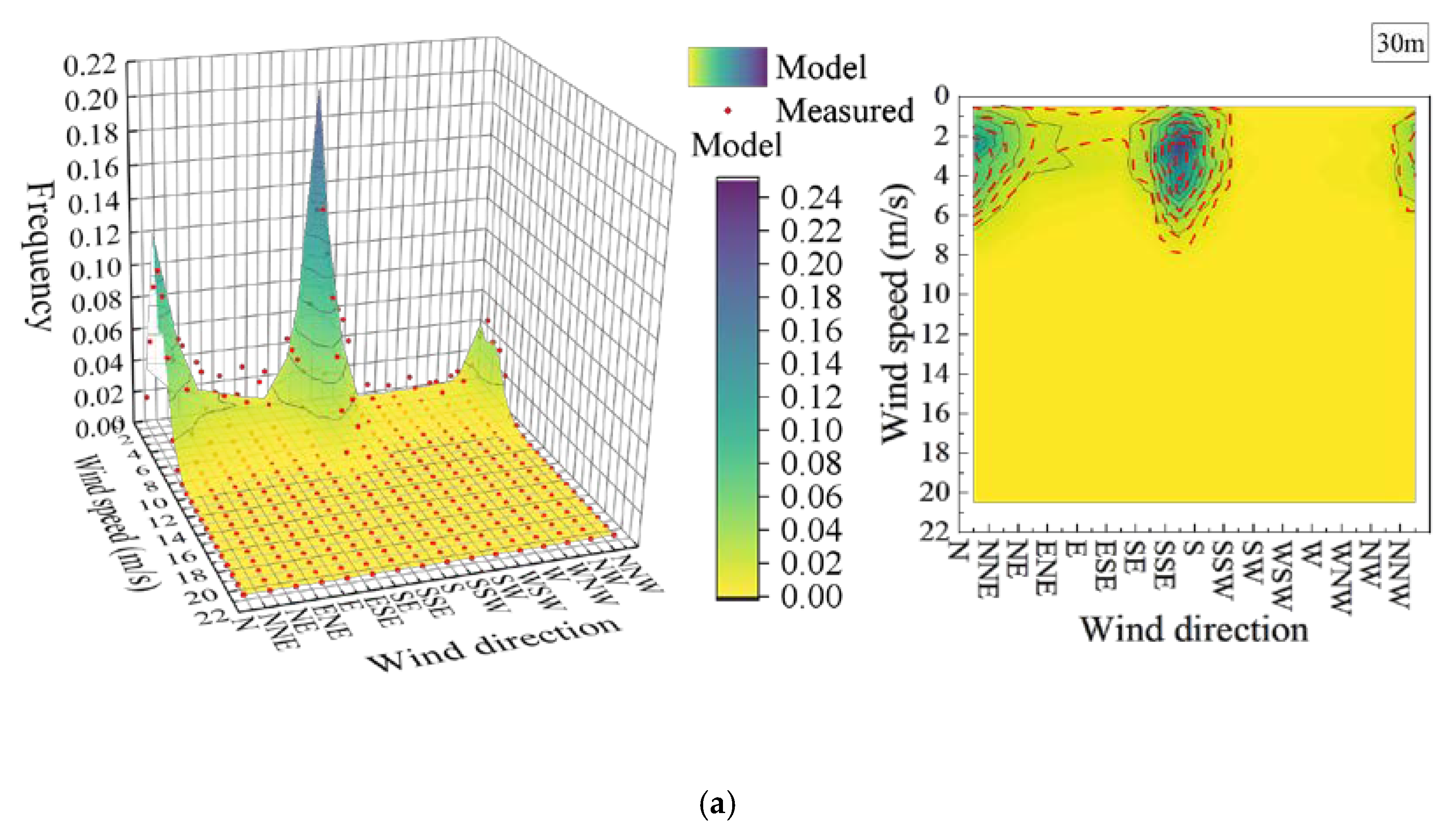
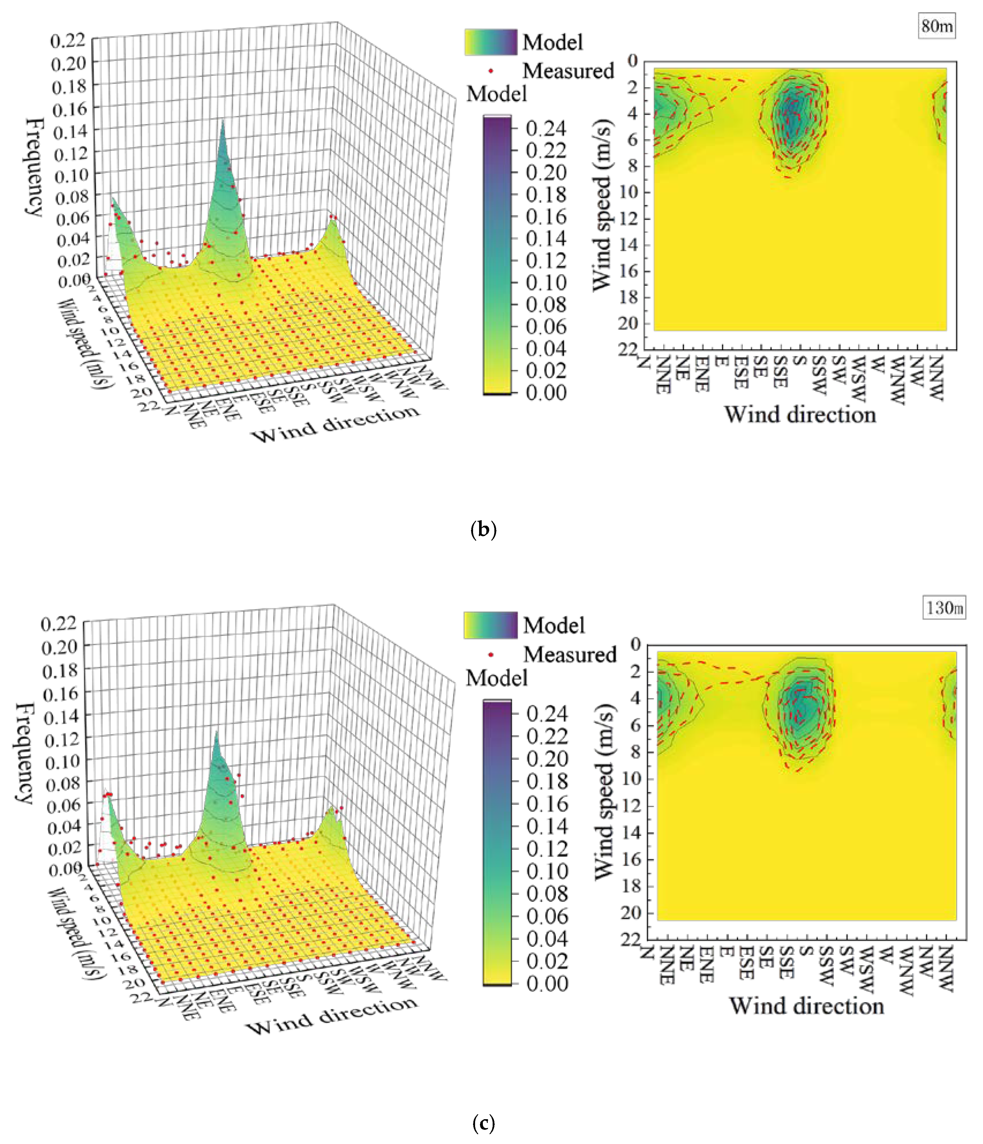
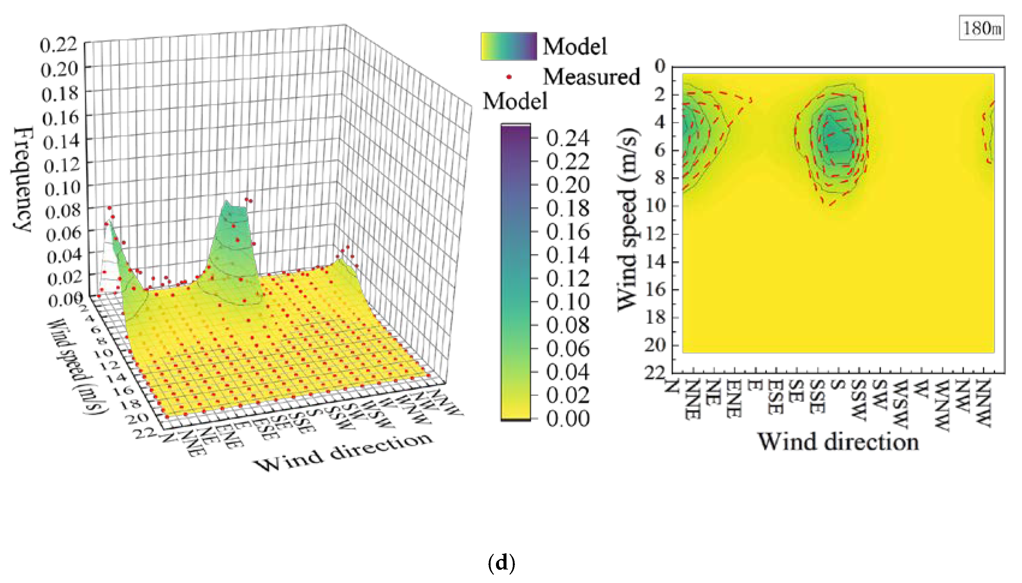
The fitting effect of the AL model is shown in Figure 6a–d. As can be seen in the figure, the probability of main wind direction decreased with an increase in height, due to the influence of the surface. The model prediction results fitted well with the measured data.

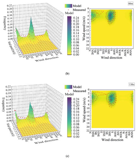
Figure 6. (a–d) AL model fitting effect.

3.3. Joint Distribution of Wind Speed and Wind Direction at Diffierent Heights

It can be seen from the expression in Table 1 that the elliptic family copula function has too many parameters. Taking the 16 heights in this paper as an example, 120 parameters would be required if this type of copula function was used, which is inconvenient for practical applications; therefore, it is recommended that the Archimedes copula function is used. In this paper, the Gumbel copula and Clayton copula functions, which can describe asymmetric correlation, are used to estimate the parameters through the maximum likelihood method. In the study, it was noted that each sample was unique, i.e., the probability of occurrence of each sample was 1/8270; therefore, CDF was used for the goodness-of-fit test in this part. The results are shown in Table 9. It can be seen that the Gumbel copula function describes the correlation of this group of wind speed samples better, so the Gumbel copula function is recommended for this group of wind speed samples. CDF of measured data and model prediction results were calculated and compared. The model’s final fitting effect is shown in Figure 7.

Table 9. Copula function parameter results and goodness of fit.

Function	θ	R2
Clayton	3.65455	0.91741
Gumbel	3.82273	0.94963

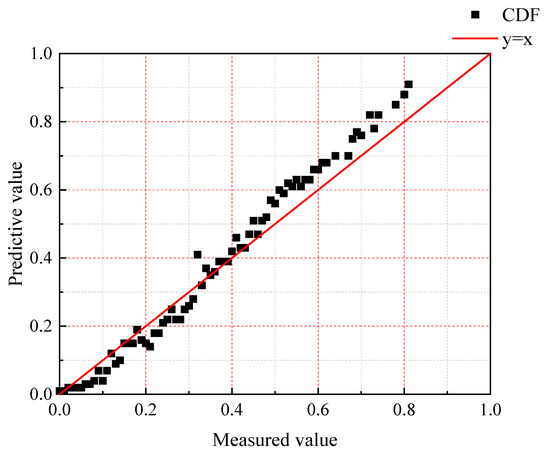
Figure 7. The AL–Copula model fitting effect.

4. Conclusions

In this paper, the formula for connecting two-dimensional distribution function with the copula function is derived and a modeling method is given for the three-dimensional joint distribution of wind speed, wind direction, and height. The method started with a one-dimensional wind speed distribution model and used mvM to describe a wind direction distribution. A two-dimensional joint distribution model of wind speed and wind direction at each height was established through the AL model. Then, the two-dimensional joint distributions at each height were connected by the copula function, from which a three-dimensional joint distribution model of wind speed, wind direction, and height was formed. Our main conclusions are as follows:

(1) The copula function can connect not only one-dimensional distribution but also two-dimensional or even multi-dimensional distribution. In practice, the joint distribution function of variables that have a clear relationship between each other can be obtained first, and then the copula function can be used to connect these joint distribution functions to form the overall joint distribution function.

(2) This kind of joint distribution model has a good fitting effect, can make full use of the original data, and is not affected by the characteristics of wind speed data. The example in this paper is based on the measured data in a flat area. Because of the compatibility of its function, it can be applied to complex terrains, such as mountain canyons, in subsequent research.

(3) The two-dimensional joint distribution model can describe the relationship between wind speed and wind direction; a suitable two-dimensional distribution model can be adopted to fit the data. The distribution model proposed in this paper can be used for three-dimensional distribution fitting. The number of different heights will not affect the establishment of a low-dimensional model. This will only affect the parameter value of the copula function. In practical applications, the influence of bad data points on the final results can be avoided.

(4) The wind speed in the area chosen for this study is in good compliance with the Weibull distribution parameters, and the north and south wind prevails in this area. In addition, the probability of prevailing wind direction decreases as height increases.

(5) The three-dimensional distribution model was used to obtain the wind field characteristics and to further calculate the wind load of the structure. It provides a basis for wind resistance design of high-rise buildings or long-span bridges. The model can also be applied to the field of wind power to evaluate the potential wind energy in a certain area.

References

- Chaurasiya, P.K.; Warudkar, V.; Ahmed, S. Wind energy development and policy in india: A review. Energy Strategy Rev. 2019, 24, 342–357. [Google Scholar] [CrossRef]
- Zheng, C.-W.; Xiao, Z.-N.; Peng, Y.-H.; Li, C.-Y.; Du, Z.-B. Rezoning global offshore wind energy resources. Renew. Energy 2018, 129, 1–11. [Google Scholar] [CrossRef]
- Caracoglia, L. Wind effects on structures: Modern structural design for wind. J. Struct. Eng. 2021, 147. [Google Scholar] [CrossRef]
- Jung, C.; Schindler, D. Wind speed distribution selection - a review of recent development and progress. Renew. Sustain. Energy Rev. 2019, 114. [Google Scholar] [CrossRef]
- Usta, I. An innovative estimation method regarding weibull parameters for wind energy applications. Energy 2016, 106, 301–314. [Google Scholar] [CrossRef]
- Wang, J.; Hu, J.; Ma, K. Wind speed probability distribution estimation and wind energy assessment. Renew. Sustain. Energy Rev. 2016, 60, 881–899. [Google Scholar] [CrossRef]
- Jung, C.; Schindler, D. Global comparison of the goodness-of-fit of wind speed distributions. Energy Convers. Manag. 2017, 133, 216–234. [Google Scholar] [CrossRef]
- Akgul, F.G.; Senoglu, B.; Arslan, T. An alternative distribution to weibull for modeling the wind speed data: Inverse weibull distribution. Energy Convers. Manag. 2016, 114, 234–240. [Google Scholar] [CrossRef]
- Arslan, T.; Acitas, S.; Senoglu, B. Generalized lindley and power lindley distributions for modeling the wind speed data. Energy Convers. Manag. 2017, 152, 300–311. [Google Scholar] [CrossRef]
- Carta, J.A.; Bueno, C.; Ramirez, P. Statistical modelling of directional wind speeds using mixtures of von mises distributions: Case study. Energy Convers. Manag. 2008, 49, 897–907. [Google Scholar] [CrossRef]
- Wang, H.; Xu, Z.; Tao, T.; Yao, C.; Li, A. Analysis on joint distribution of wind speed and direction on sutong bridge based on measured data from 2008 to 2015. J. Southeast Univ. (Nat. Sci. Ed.) 2016, 46, 836–841. [Google Scholar] [CrossRef]
- Ye, X.W.; Xi, P.S.; Nagode, M. Extension of rebmix algorithm to von mises parametric family for modeling joint distribution of wind speed and direction. Eng. Struct. 2019, 183, 1134–1145. [Google Scholar] [CrossRef]
- Han, Q.; Hao, Z.; Hu, T.; Chu, F. Non-parametric models for joint probabilistic distributions of wind speed and direction data. Renew. Energy 2018, 126, 1032–1042. [Google Scholar] [CrossRef] [Green Version]
- Zheng, X.; Li, H.; Li, C.; Liu, Y.; Zhang, H. Joint probability distribution and application of wind speed and direction based on multiplication rule and al model. Eng. Mech. 2019, 36, 50–57, 85. [Google Scholar]
- Dong, S.; Lin, Y. Study of joint probabilistic distribution of wind speed and direction at a fixed observation station. Eng. Mech. 2016, 33, 234–241. [Google Scholar]
- Lin, Y.; Dong, S. Study of seasonal change of the extreme wind speed at zhifudao observation station considering wind direction distribution. Period. Ocean Univ. China 2018, 48, 132–139. [Google Scholar]
- Diaz, G.; Casielles, P.G.; Coto, J. Simulation of spatially correlated wind power in small geographic areas-sampling methods and evaluation. Int. J. Electr. Power Energy Syst. 2014, 63, 513–522. [Google Scholar] [CrossRef] [Green Version]
- Lou, W.; Zhang, L.; Huang, M.F.; Li, Q.S. Multiobjective equivalent static wind loads on complex tall buildings using non-gaussian peak factors. J. Struct. Eng. 2015, 141. [Google Scholar] [CrossRef]
- Li, Y.; Hu, P.; Xu, X.; Qiu, J. Wind characteristics at bridge site in a deep-cutting gorge by wind tunnel test. J. Wind Eng. Ind. Aerodyn. 2017, 160, 30–46. [Google Scholar] [CrossRef]
- Bai, H.; Li, J.; Liu, J. Experimental study on wind field characteristics of sanshui river bridge site located in west valley region. J. Vib. Shock 2012, 31, 74–78. [Google Scholar]
- Sklar, A. Fonctions de Repartition a n Dimensions et Leurs Marges; Publications de l’Institut de Statistique de l’Université de Paris: Paris, France, 1959; Volume 8, pp. 229–231. [Google Scholar]
- Nelsen, R. An introduction to Copulas; Springer: New York, NY, USA, 2006. [Google Scholar]
- Gilenko, E.; Chernova, A. Saving behavior and financial literacy of russian high school students: An application of a copula-based bivariate probit-regression approach. Child. Youth Serv. Rev. 2021, 127, 106122. [Google Scholar] [CrossRef]
- Kumar, S.; Tiwari, A.K.; Raheem, I.D.; Hille, E. Time-varying dependence structure between oil and agricultural commodity markets: A dependence-switching covar copula approach. Resources Policy 2021, 72, 102049. [Google Scholar] [CrossRef]
- Wang, L.; Xu, T. Bidirectional risk spillovers between exchange rate of emerging market countries and international crude oil price-based on time-varing copula-covar. Comput. Econ. 2021, 1–32. [Google Scholar] [CrossRef]
- Johnson, R.A.; Wehrly, T.E. Some angular-linear distributions and related regression models. J. Am. Stat. Assoc. 1978, 73, 602–606. [Google Scholar] [CrossRef]
Publisher’s Note: MDPI stays neutral with regard to jurisdictional claims in published maps and institutional affiliations. |
© 2021 by the authors. Licensee MDPI, Basel, Switzerland. This article is an open access article distributed under the terms and conditions of the Creative Commons Attribution (CC BY) license (https://creativecommons.org/licenses/by/4.0/).