Article

Explaining Bad Forecasts in Global Time Series Models

1
Jožef Stefan Institute, Jamova 39, 1000 Ljubljana, Slovenia
2
Qlector d.o.o., Rovšnikova 7, 1000 Ljubljana, Slovenia
3
Jožef Stefan International Postgraduate School, Jamova 39, 1000 Ljubljana, Slovenia
4
Faculty of Electrical Engineering, University of Ljubljana, Tržaška 25, 1000 Ljubljana, Slovenia
*
Author to whom correspondence should be addressed.
Appl. Sci. 2021, 11(19), 9243; https://doi.org/10.3390/app11199243
Submission received: 9 August 2021 / Revised: 23 September 2021 / Accepted: 24 September 2021 / Published: 4 October 2021
(This article belongs to the Special Issue Explainable Artificial Intelligence (XAI))

Abstract

:

Featured Application

The outcomes of this work can be applied to understand better when and why global time series forecasting models issue incorrect predictions and iteratively groom the dataset to enhance the models’ performance.

Abstract

While increasing empirical evidence suggests that global time series forecasting models can achieve better forecasting performance than local ones, there is a research void regarding when and why the global models fail to provide a good forecast. This paper uses anomaly detection algorithms and explainable artificial intelligence (XAI) to answer when and why a forecast should not be trusted. To address this issue, a dashboard was built to inform the user regarding (i) the relevance of the features for that particular forecast, (ii) which training samples most likely influenced the forecast outcome, (iii) why the forecast is considered an outlier, and (iv) provide a range of counterfactual examples to understand how value changes in the feature vector can lead to a different outcome. Moreover, a modular architecture and a methodology were developed to iteratively remove noisy data instances from the train set, to enhance the overall global time series forecasting model performance. Finally, to test the effectiveness of the proposed approach, it was validated on two publicly available real-world datasets.

1. Introduction

Time series forecasting is a relevant problem with application in many domains [1], gaining further relevance with the increasing availability of historical data [2]. Historically, much research focused on time series models trained on a single time series [3]. Though global machine learning models issued good results in the past, they gained new attention with the advent of deep learning [4], and recent success on the M4 and M5 time series forecasting competitions [5,6]. Such models can learn patterns shared across multiple time series, enhancing the overall forecasting performance. The usage of multiple time series to train the model can be considered a source of explainability: each forecast can be explained not only through past behavior on a single time series, but similar patterns can be found in other time series, providing a different perspective and complementary insights [7]. The ability to develop global time series models implicates scaling advantages too: it reduces the number of forecasting models, and thus the amount of human supervision required to build them, and fewer deployments, monitoring, and maintenance [8].
While authors have shown that global time series machine learning forecasting models (GTSMLFM) can achieve better performance overall, “understanding when and why global forecasting models work, is arguably the most important open problem currently in time series forecasting” [3]. It is thus crucial to develop Explainable Artificial Intelligence (XAI) approaches to answer those questions. The approaches can differ based on the goal they aim to tackle (e.g., increase trust in the model or provide insights that can be used to improve the model), the user profile they target and focus (if the explanations provided are either local or global) [9].
The paper focuses on understanding when and why GTSMLFMs work, providing relevant information to the end-users and the machine learning engineers. The end-users must understand if a particular forecast instance can be relied upon (e.g., detect if it can be considered anomalous) and what features do influence the forecast. If the forecast is anomalous, the user can be interested in getting to know some counterfactual examples. While machine learning engineers will appreciate this information, they can also find which instances from the train set most likely influenced the models’ learning to issue an unlikely forecast. To provide such an understanding to the users, we use local features relevance, anomaly detection models, and develop a novel approach to provide counterfactual explanations for regression methods. Furthermore, we integrate the insights into a dashboard that can serve the end-users and the machine learning engineers, to understand better when and why global time series forecasting models work.
This research provides several contributions, with which we address the gap of providing means to answer when and why a GTSMLFM prediction should be considered a bad forecast [3]. First, we make use of anomaly detection algorithms to identify potentially wrong forecasts. Then, we compute the models’ feature attribution for those data instances, identify similar data instances in the train set, and create counterfactual examples. Furthermore, we develop a dashboard integrating the insights mentioned above and a line plot showing the time series, with a relevance heatmap overlay to inform the influence of data points on a given forecast. While such relevant heatmaps have been widely applied for deep learning models, they are not frequently used for other time series models. In addition, such a dashboard enables a visual inspection of time series and forecasts—a valuable tool for end-users and machine learning engineers. Finally, based on our experience, we outline an architecture and a methodology that can be followed to enhance the dataset and GTSMLFMs iteratively.
To evaluate our approach, we conduct a series of experiments and perform a quantitative evaluation to measure the impact of the insights are developed when engineering the GTSMLFM. In particular, we measure the Mean Absolute Scaled Error (MASE) [10], the number of outliers observed in the test set, and the number of instances removed from the train set, based on the detected anomalous predictions.
We organized the remainder of this paper as follows. In Section 2, we review related scientific works; in Section 3, we introduce the proposed architecture, while in Section 4, we provide details on the methodology that we followed to treat the dataset and train new GTSMLFMs iteratively. In Section 5, we describe two different time series datasets that we used to test our approach, detailing the preprocessing steps and features that we created. In Section 6, we describe the experiments that we performed, provide a more detailed overview regarding the metrics used to measure the results, and the results we obtained, while in Section 7 we address the limitations of this research. Finally, in Section 8, we conclude by summarizing this research, and outline future work.

2. Review of Related Scientific Works

2.1. Forecasting Time Series: Local vs. Global Approach

For many decades, most research on time series forecasting assumed that the time series are generated by independent processes and can be tackled as a regression problem, creating a single model per time series (local models) [8,11]. Growing empirical evidence suggests that creating a single model to forecast multiple time series (under the assumption of forecasts’ independence for different time series) known as global models can outperform local ones. Seminal research on using global models developed decades ago [12], and the concept was further explored by many researchers afterwards [13]. The first approaches towards global models considered pooling similar time series, which improves the overall models’ accuracy. By having more training data of similar time series, algorithms can better distinguish common data patterns, while also minimizing distortions introduced by outlier data points [14]. On the other side, this approach requires defining some time series grouping criteria, which can lead to suboptimal groupings [15]. Among pooling strategies, we can find model-based clustering [14,16,17], random clustering [8], grouping based on similarity measures [18,19,20], or expert judgement [21]. Recent research has explored creating global models considering all available time series, regardless of their heterogeneity, obtaining promising results [3,8,22]. Furthermore, it has been demonstrated that, for every dataset, some global model exists that can equal or outperform a local model, regardless of how heterogeneous the data may be [8]. Such models make the strong assumption that some relationship exists between time series, though the forecasts are independent of each other [11].
These insights, the good results obtained by applying global neural network models for time series forecasting [11,23,24,25,26,27], and success of global models at the M4 and M5 competitions [5,6], have renewed the research interest on global models for time series forecasting [3]. In such models, the relationship between time series is not very well understood, and understanding why and when do global time series forecasting models work remains an open research topic [3]. We envision that anomaly detection algorithms can be used to detect when the GTSMLFM provides accurate forecasts or not, and XAI approaches can provide insights to understand better factors affecting the forecasts, and provide prototype (local) explanations [28], and counterfactual examples.

2.2. Time Series Anomaly Detection

One of the open research questions regarding GTSMLFM is, when do such models provide acceptable forecasts [3]? Such response can be obtained from anomaly detection algorithms and models, which can alert on point anomalies. In this section, we provide an overview of anomaly detection techniques, focusing on the ones developed and applied in a time series setting. We use the terms anomaly, outlier, or deviant interchangeably [29], to denote “observations that deviate so much from others as to arouse suspicion that it was generated by another mechanism” [30]. In particular, outliers related to time series data must also consider the behavior across time [31].
Outliers can be characterized into many types. The first characterization of this type can be found in [32], who introduced the concepts of two time series’ outlier types: those (a) that affect a single observation (type I), and those (b) that affect an observation and the subsequent ones (type II). More recently, [31] distinguishes between point outliers (single point in the time series, which has an unusual value when compared to the whole time series or the neighboring points) and subsequence outliers (points which may not be outliers by themselves, but the sequence arrangement is anomalous). Subsequence outliers are further classified into contextual anomalies (they are anomalous in the context of the surrounding observations) or pattern anomalies (they are anomalous regardless of the surrounding observations) [33]. In this research, we limit ourselves to point outliers.
Anomaly detection techniques are frequently classified into three categories: statistical, distance-based approaches, and model-based approaches [34]. The first anomaly detection techniques were developed in statistics and remained among the most frequently used ones. Non-parametric techniques usually allow fast computations and are adopted where such speed is of primary importance. Among them, we find the histogram-based approaches, which assume feature independence and determine the outliers based on the histogram distribution [35,36,37,38]. Other non-parametric approaches are bitmap time series anomaly detectors, which compute the relative frequency of its features to create a bitmap and identify anomalous time series [39,40], and statistical methods that allow estimating outliers based on a kernel density estimation by using a kernel function. Such kernel functions can provide a probability estimate, given that function is a probability density function [34,41,42,43]. Among the parametric methods, we find the Gaussian methods, such as box-plot anomaly detection [44], the Gaussian process [45,46], or regression approaches such as least squares regression [47,48,49].
Statistical anomaly detection methods cannot be applied on datasets with an unknown distribution [38]. Different approaches were developed to overcome this issue. When considering the distance between data points, we find the k-nearest-neighbors (kNN), which determines the outliers based on the kNN distance. While approaches were developed to determine the best k parameter [50], some techniques attempted to avoid dependence on the k-value. One such method is the local outlier factor (LOF) method, which computes the distance from a point to all other points in the dataset [51]. A similar approach was followed at the outlier detection using indegree number (ODIN), which computes the number of instances that contain a given point in their neighborhood. However, a parameter is required to determine the outlier threshold [52]. A different method was developed by [53], who introduced the multi-granularity deviation factor to identify local density variations that lead to isolated outliers or outlying clusters. Variations to the LOF method were developed to solve some of its shortcomings. For example, the connectivity-based outlier factor (COF) aims to capture better clusters where the data points are distributed in a linear manner [54], while influenced outlierness (INFLO) attempts to better discriminate points nearby two clusters with different densities [55]. Finally, to account for the different feature importance, [56] developed an alternative anomaly detection algorithm, using a weighted kNN.
Model-based techniques can be divided into (i) models that learn and predict whether the value is anomalous and (ii) models that compare the potential outlier with expected values drawn from a generative model or data distribution. Since model-based techniques require labeled data, active learning can be utilized to minimize the labeling effort [57]. Among the models of the first group, we find the SVM-based models, such as the one-class support vector machine (OC-SVM), which was introduced by [58], and later enhanced by many authors [59,60]. Since the regular SVM algorithm can provide poor generalization on an imbalanced dataset, the authors suggested representing the anomalous classes with the high dimensional space origin and mapping anomalous instances close to it. Other SVM variants used for anomaly detection include support vector data description (SVDD) [61], and SVM-SVDD [62]. A different intuition is followed in the Isolation Forest. This tree-based model is based on the principle that the fewer instances of anomalies generate a smaller number of partitions, and thus are likely to have short paths in the tree structure [63]. Other models reported in the literature involve the use of random forests [64], gradient boosted machines [65], artificial neural networks [66], or voting ensembles [67]. Models from the second group have multiple configurations, varying the generative methods and outlier detection criteria. Some examples are the use of ARIMA models to predict future time series values and mark incoming readings as anomalies if they exceed a certain threshold when compared with the forecast [68,69]. Other approaches fused statistical methods and ANNs [70], or used ANNs alone [31,71].
Anomaly detection algorithms can identify anomalous forecasts in the context of a particular time series. Based on the algorithm type, insights can be gained on why the point forecast is considered anomalous. Additional insights can be obtained through XAI to understand which features were most influential to such forecast and provide counterfactual examples, highlighting value changes to those features that would produce a better outcome.

2.3. Explainable Artificial Intelligence

The increasing adoption of artificial intelligence demands understanding the logic beneath the forecasts so that a decision can be made as to whether such forecasts can be trusted or not [72]. The sub-field of artificial intelligence devoted to research on obtaining and providing such understanding is called explainable artificial intelligence (XAI). Authors identify two sources of model opacity [73]. The first one is the complexity of the formal structure of the model, which can be beyond human comprehension, or alien to human reasoning. When the opacity cannot be removed even by human experts, we speak about deep opacity [74]. The second source of opacity is the intentionally induced opaqueness to avoid revealing sensitive model details (e.g., due to their proprietary nature).
Researchers developed multiple approaches to provide black-box explanations of forecasting models. Among the most frequently cited, we find LIME [75] and its variants (e.g., k-LIME [76], DLIME [77], and LIMEtree [78]), Anchors [79], Local Foil Trees [80], or LoRE [81]. These approaches build surrogate models for each prediction sample, learning the reference model’s behavior on the particular case of interest by introducing perturbations to the feature vector variables. The Shapley additive explanations take a different approach (SHAP) [82,83], which are grounded in cooperative game theory. The feature relevance is computed based on the approximate computation of Shapley values. Shapley values are also used to explain features relevance in a time series setting. In particular, the TimeSHAP implementation measures which features and past events are most relevant to a recurrent model [84].
Research regarding XAI for time series has focused mainly on explainability for deep learning models. One of the first of such methods was introduced by [85], who computed feature attributions by taking the partial derivative of the output class with respect to the input. This method was later improved in the Gradient*Input method, which computes neuron and filter activations for a specific instance by multiplying the input by the partial derivative of a layer with respect to the input [86]. Similar approaches followed, such as the Deep Learning Important FeaTures (DeepLIFT) [87], integrated gradients [88], or Smooth-Grad [89]. The introduction of attention mechanisms to deep learning models was also envisioned as a source of explainability, since it provides insights regarding which points in time are relevant to the forecast [90]. Such information is frequently presented in heatmaps [91,92], saliency maps [85,93], and custom visualizations [94]. Finally, several feature perturbation methods were developed to measure the features’ contribution to the forecasted value when such features are removed [95], or masked [96,97,98].
Methods such as Shapley values [99] and region partition trees [100] have been successfully applied to explain detected anomalies. More systemic approaches have been developed too, such as Exathlon [101], EXAD [102], and others [103]. While EXAD focuses on explanation discovery for each anomaly, Exathlon crafts the explanations, providing two pieces of information to the user: why the data point was identified as an anomaly and the root causes of such anomaly.
Along with feature relevance, it is sometimes important to know how values should change to achieve a different forecast. Such examples are known as counterfactual explanations. When counterfactual explanations are provided as actionable advice, they are known as directive explanations. Directive explanations can be either directive-specific (suggest a concrete action to change the forecasted value), or directive-generic (suggest a generic action to alter the forecasted value) [104]. While most frequently applied to classification models, counterfactual explanations are also applied to regression models. While such counterfactual explanations most frequently use some threshold [105], other implementations were developed based on potentials [106], or satisfiability modulo theories solvers [107], among others.
While counterfactual examples provide value to understand how to change a certain target state, sometimes it is useful to visualize prototypical instances similar to the feature vector used to issue a prediction. Such examples are known as prototype explanations, and allow us to understand better which instances influenced a certain forecast [108].
As described above, multiple methods exist to obtain relevant information that can explain the underlying reasoning of an artificial intelligence model. Along with them, it is also important to consider how such information is presented to the users. Good explanations should convey meaningful information, resemble a logic explanation [109], target a specific user profile [110], focus on actionability, and if possible, provide some counterfactual examples [111]. An explanation should take into account relevant context, which can be captured in three elements: the target user profile, the explanation goals (e.g., improve the model, or enhance trust in the system), and the focus (if the explanations provided are meant at a global or local level).
When developing our architecture and dashboard, we considered different intuitive ways to present the information, ranging from plots and tables to human-readable sentences. When the forecasts are considered anomalous, it is helpful to the user to understand why such a forecast is considered anomalous, which are the most relevant features to that forecast, provide counterfactual examples, and examples from the training set that could have influenced the forecast.

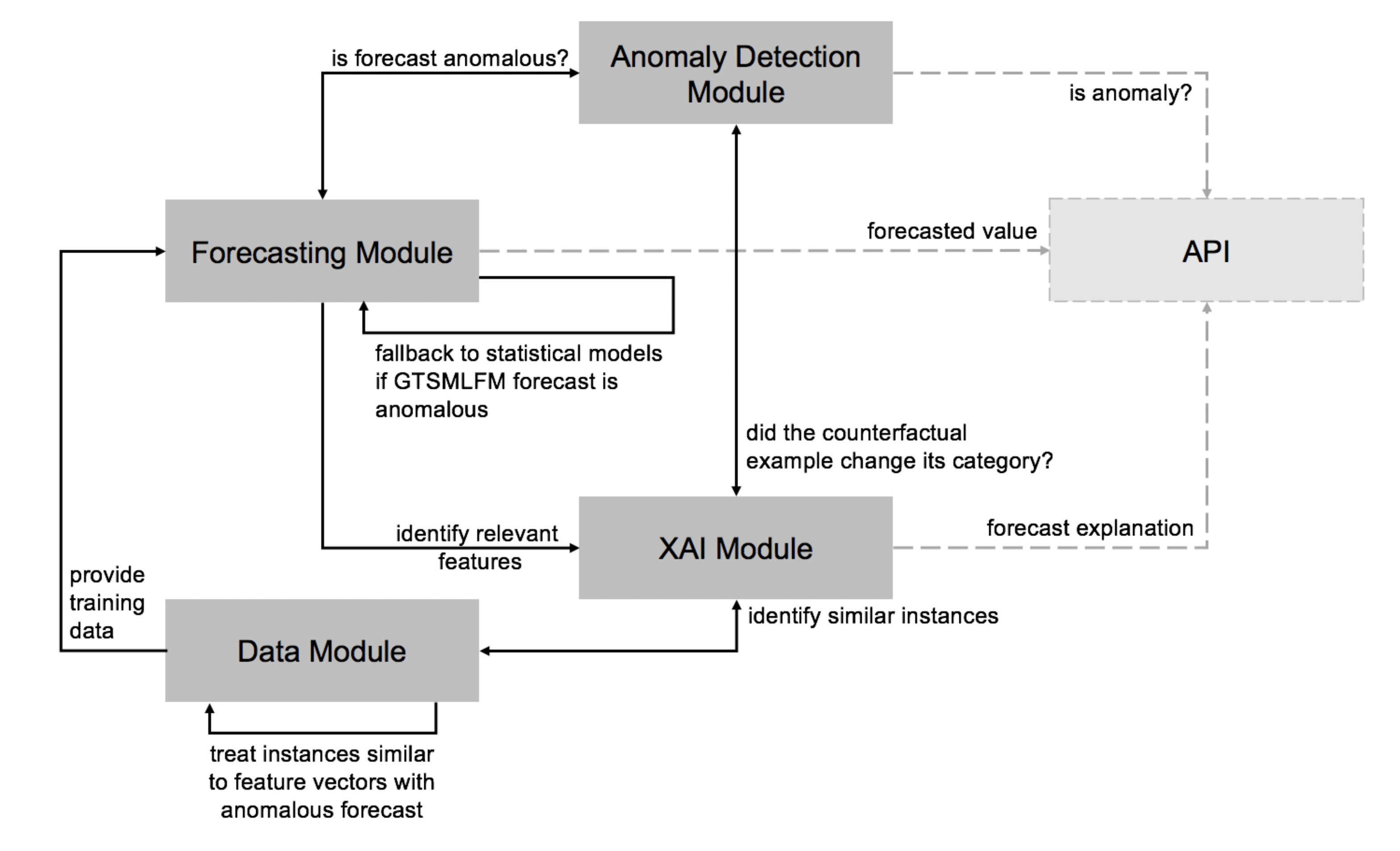
3. The Proposed Architecture

We propose a modular architecture to provide forecast explanations for global time series forecasting models. We combine anomaly detection and explainability methods to enhance the forecasting precision and provide valuable contextual information to the end-users. The anomaly detection module provides a means to identify potentially bad forecasts. In such cases, we can fall back to a local statistical model, or alert the user that a given forecast should not be trusted given past time series’ behavior. The feature relevance informs the user on which variables exercised the most influence on the forecast. We use them as an input when computing the counterfactual examples to understand better what value changes on those variables would produce an outcome that is no longer considered an outlier. Finally, we provide insight to the user on which data instances could have influenced the forecasting models to provide such a forecast by identifying them in the train set based on their similarity regarding the forecasted one. We consider that this information helps investigate possible patterns learned by the model and how to engineer a better model learning in the future.
The architecture (see Figure 1) comprises the following components:
  • Data Module: provides a dataset to train machine learning GTSMLFMs. The dataset comprises time series data, either considering their raw values and derivative features or a refined version where specific instances that could cause outlier forecasts were treated. The module wraps a set of strategies to find and treat data instances that are similar to the ones producing outlier forecasts, identified by the anomaly detection module.
  • Forecasting Module: comprises a machine learning GTSMLFM, and a set of local statistical models to forecast the time series. The machine learning GTSMLFM is created based on a dataset obtained from the Data Module. The Forecasting Module makes use of the input provided by the Anomaly Detection Module to decide whether the outcome should be the forecast obtained from a GTSMLFM, or a local statistical model.
  • Anomaly Detection Module: leverages algorithms and models to analyze the forecast in the context of a time series and classify it as an anomaly or not. It interacts with the Forecasting Module and the XAI Module, providing feedback on whether a forecast can be considered anomalous or not.
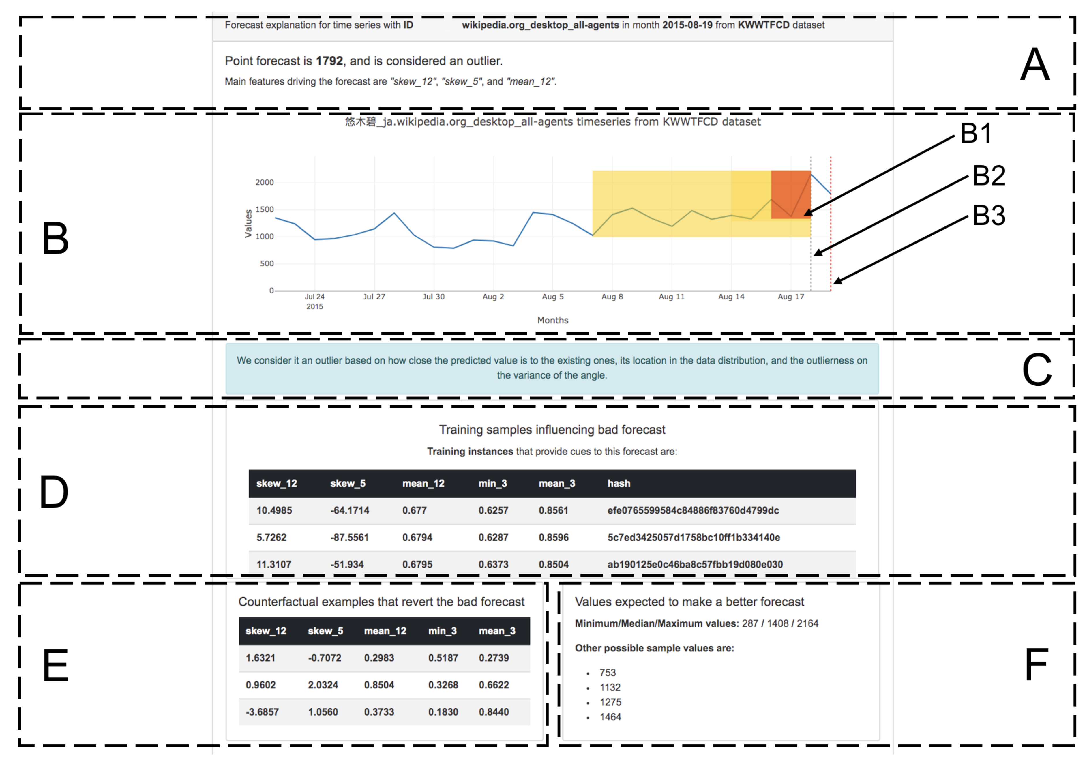
  • XAI Module: uses various XAI algorithms and models to craft forecast explanations for the user. In particular, we envision that this module (i) indicates if the forecast is anomalous, (ii) crafts a text explanation highlighting most relevant features influencing a specific forecast, (iii) shows a sample of n data instances found in the train set that most likely influenced the GTSMLFM towards the given forecast, and (iv) shows a set of counterfactual examples created considering (a) the relevant features to that specific forecast, and (b) past values observed for that particular time series. We consider that this information provides the user a good insight into whether the forecast can be trusted and understand the behavior of the underlying model.
  • API: a standard Application Programming Interface (API) endpoint can be used to serve the user as a front-facing interface, masking the structure, complexity, and deployment configuration of each of the modules mentioned above.
The architecture was implemented in a prototype application for the purpose of this paper, and not deployed into production. The backend was built using the Python 3.6 language, and leveraging multiple open-source data processing and machine learning libraries (Numpy [112], Pandas [113], Scikit-Learn [114], Scipy [115], Lime [75], Pyod [116], LightGBM [117]), and exposing relevant data through an HTTP REST API, using the Flask framework [118]. To build the frontend, we used HTML to layout the core of the dashboard, the Bootstrap framework to embellish the user interface, Plotly-js [119] to draw the plot, and jQuery [120] to interface with the HTTP REST API, retrieving the data and serving the content to the web page.
The interaction between the modules embodies the methodology we followed to enhance the GTSMLFM performance iteratively and provide an insight to the user regarding when and why does a GTSMLFM model provides an adequate forecast or not. We detail the methodology in Section 4.

4. Methodology

In this section, we describe how we leveraged the information provided by a prototype application built following the architecture described in Section 3, to enhance a GTSMLFM. To that end, we developed an iterative methodology inspired by work done by several authors, and summarized in Fig. Figure 2. Scientific literature on GTSMLFMs agrees that pooling similar time series does provide an advantage over local models [3,4,13,21], while pooling and time series similarity criteria remain an arbitrary choice [15]. Furthermore, some research indicates that GTSMLFMs can be trained over disparate time series and still obtain good forecasting results. We propose training an initial model over all the time series and measuring its performance. We then identify anomalous forecasted values. We consider that these values are a consequence of a subset of train data instances with a similar feature vector but different target values. To identify such instances, we first compute the feature relevance for a particular forecast. Given the N most relevant features to that forecast, we search for similar instances in the train set computing the cosine distance across the feature vectors, considering only the subset of the aforementioned N features. To avoid distortions due to different feature magnitudes, we scaled the features between zero and one. To decide which train instances to remove, we set an arbitrary similarity threshold. It is important to consider that the GTSMLFM performance can be affected by train data instances that lead to learning inaccurate forecasting patterns and the amount of data available, which can eventually lead to better predictions. Thus, setting the right threshold requires a compromise between both factors and can be subject to trial and error. To conclude an iteration, we assess the GTSMLFM quality. In particular, we decided to measure it through three metrics (see Section 6): (i) mean absolute scaled error (MASE) [10], (ii) the number of outliers detected in the test set, and (iii) the number of train instances removed from the dataset to train that particular GTSMLFM. Following the Equation (1) [28], we argue that, while local statistical models do not match the overall performance of a good GTSMLFM, they can sometimes provide a better prediction when the GTSMLFM provides an anomalous forecast. To retain the scaling advantages, such as ease of deployment, and avoid dedicating human resources to developing and maintaining such models, simple heuristics such as the näive forecast, simple moving average, or exponential smoothing can be used.
Data = Global Model + Local Models + Noise
The equation represents that local models can make better forecasts when the global model fails to predict reasonably. The equation was reproduced from [28].
Once we finalize an iteration, we start a new one by retraining the GTSMLFM on the new dataset, following the steps mentioned above. Iterative model retraining is based on the RemOve And Retrain (ROAR) method [121], developed to identify features relevance measuring the model performance change between iterations when a feature is nullified. In our case, we do not measure the impact of the features but of a subset of training instances when removed from the dataset. Furthermore, inspiration to look into training instances to understand their impact on a given forecast was obtained from [122], who did so using influence functions.

5. Case Study

In this research, we considered two open datasets that are widely used in time series forecasting research: M4 competition dataset (M4CD) [5], and the Kaggle Wikipedia Web Traffic forecasting competition dataset (KWWTFCD) [123]. To ensure that the performance of the global models does not depend on the knowledge of a particular domain or characteristics of the time series data, we defined the same set of generic features for both cases. In this section, we describe the characteristics of each dataset, provide details on how we sampled instances from them, and the preprocessing steps we performed before training the GTSMLFM.
The M4CD comprises 100,000 time series selected from the ForeDeCk database, corresponding to multiple business domains, such as industries, government, transport, household, and natural resources. While the dataset includes time series at different frequencies (from hourly to yearly frequency), we focused on those provided monthly, which account for 48,000 time series. When analyzing their metadata and the actual time series length, we found some discrepancies. We clarified them with the authors from [124], who researched how representative it is of the reality. In private correspondence, the authors confirmed that such discrepancies existed, attributing them to the original public sources from which they were obtained. Since such time series represented only a tiny proportion of the total dataset, we ignored them.
The KWWTFCD was provided by Google and introduced in a Kaggle competition in 2017. The dataset comprises time series accounting for the daily views of approximately 145,000 Wikipedia articles, starting from 1 July 2015, until 11 September 2017. The dataset distinguishes between zero and missing values.
We randomly sampled 2000 time series for each dataset and selected only a subsequence to minimize the number of missing values (first 45 values for M4CD and first 56 values for the KWWTFCD). We considered 2000 time series as a big enough sample to evaluate diverse time series and provide meaningful results, while avoiding processing the whole dataset. The need for sampling is grounded in the fact that a feature vector is created per time step for each time series, requiring extensive computational resources and time to train the models.
When designing the experiment, we considered that a global model is more likely to produce anomalous forecasts if trained over a dataset that contains two types of time series: (i) the ones whose values remain in the same order of magnitude, and (ii) the ones whose values comprehend different orders of magnitude (TSDM). We thus analyzed the proportion of time series with such properties in each dataset and ensured that the sampling respected those proportions. The new datasets comprised 903 of type (i) and 1097 of type (ii) time series for the M4CD, and 512 type (i) and 1488 type (ii) time series for the KWWTFCD. We provide further details on the original and reduced dataset in Table 1, and describe the target values distribution in Figure 3.
To describe the time series, we created a set of features, presented in Table 2. We considered three types of features: (i) the features that describe the values observed for a given time series (e.g., minimum, mean, median values, along with the standard deviation), (ii) the features that describe the time series shape (e.g., skew, kurtosis, the number of peaks we observed, and the number of values above the mean), and (iii) the features that describe the context close to the forecasted value (e.g., last observed value—which can be used as a näive forecast). We compute thirty-three features for each dataset. For the global models, we do not perform feature selection, given that in all cases, we observe the number of features satisfies the Equation (2), as suggested in [125]. For the local machine learning models, we perform feature selection selecting top K features based on their mutual information [126].
k N
k represents the maximum number of features used to train a model to avoid overfitting. N represents the number of data instances available in the train set. The equation is based on research done by [125].
Several kinds of preprocessing have been tried for GTSMLFMs in the scientific literature. Smyl [127] applied on the fly preprocessing to remove level and seasonality components. Rabanser et al. [128] found that binning proved to be useful in almost all the cases they analyzed. Duncan et al. [13] understands that differences in magnitudes and variances can be removed, either by standardizing the time series or using dimensionless dependent variables. Hewamalage et al. [129] describe applying a local normalization, deseasonalization, and log transformation to the features. Finally, Salinas et al. [27] describes scaling the features by their average value. In our case, we opted to scale the values of a feature vector between zero and one by dividing the entries by the maximum value observed in the period of interest. Such scaling forced most feature values to a standard interval between zero and one, helping the model learn similar patterns, regardless of the original time series magnitudes. To further ease the learning process to the model, we scaled the target values too.
Outlier detection was performed considering a time series comprised of the original time series data points up to the start of the forecasting horizon and then adding the forecasted value, since we only performed one step ahead forecasts (see Figure 4). Doing so enables us to use multiple anomaly detection approaches to evaluate aspects under which a particular value can be considered an outlier within the time series.

6. Experiments, Results, and Analysis

To validate the architecture and methodology described in Section 3 and Section 4, we conducted a series of experiments (summarized in Table 3) comparing four models (described in Table 4) on the reduced version of two open datasets presented in Section 5. We built our local and global forecasting model with a gradient boosted machine regressor (GBMR) [117], considering that all but one of the top five solutions of the M5 forecasting competition were based on it [6]. We configured the GBMR model to be deterministic, have a maximum depth of five, and at most a hundred estimators. All GBMR models were instantiated with the same random seed (using the value 744) and an L2 loss. For every time series, we also created two simple local statistical models: a simple moving average, based on the last three points of data, and a näive forecast, providing a forecast based on the last observed value. On top of the models we described, we built an additional model, which considered the predictions issued by the GM(GBMR) model, and used the nïve model to issue fallback predictions when detecting an anomalous prediction was given by the global model. We opted to use a näive model as fallback, since it is considered a baseline model in most of timeseries literature. In addition, the näive model is cheap to compute, and requires no previous knowledge regarding specific timeseries, making it a more scalable solution. We evaluated the models performing a nested cross-validation [130] over the last twelve data points (a year of data monthly) for M4CD and the last fourteen data points (two weeks of data daily) for KWWTFCD.
To evaluate the experiments, we considered three groups of metrics. First, we used MASE [10] to measure the model’s performance. The MASE metric provides a magnitude agnostic estimate of the forecasting precision achieved by the model, comparing the model’s performance against a nïve forecast. We measured the MASE values for the MA(3), GM(GBMR), GM(GBMR)+näive, and LM(GBMR) models. Second, we assessed the anomalies detected in the test set. We measured (i) how many GM(GBMR) predictions were considered anomalous when the target values were not (GM(GBMR) vs. Target discrepancy column in Table 5); (ii) how many target values were identified as anomalous (Target column in Table 5); (iii) how many GM(GBMR) predictions were identified as anomalous, and their overlap regarding the GM(GBMR) column under Anomalies in test in Table 5); and (iv) how many GM(GBMR)+näive predictions were identified as anomalous, and their overlap regarding the GM(GBMR)+näive column under Anomalies in test in Table 5). Finally, we measured how many instances were erased from the train set based on their similarity to feature vectors producing anomalous forecasts. Through these sets of metrics, we could assess the model’s performance when changing the experimental conditions, understand if the detected outliers correspond to true or false positives, and how successfully does the global model behave in such cases, and if there is any correlation between the number of train instances removed and the global model’s performance.

6.1. Premise Validation (Experiment 1)

We devoted the first experiment to validate the premise of this work: that the global model outperformed the local ones (GM(GBMR) vs. MA(3) and LM(GBMR) in Experiment 1), and even the GM(GBMR)+näive, showing that the fallback to the näive forecast did not provide the expected performance improvements. This was confirmed in the rest of the experiments. Our intuition behind the result is that fallback forecasts replacing the original prediction in false positives issued by the anomaly detector (for which the GM(GBMR) model would have a better prediction) degrade the overall performance and lead to suboptimal results. We then performed four additional experiments to understand if removing instances from the train set similar to the reference vector generating an anomalous forecast could improve the performance of the global model.
It must be noted that the anomaly detection is run on forecasted values. Thus, while anomalies can be subjective, we consider that objective criteria can be established to identify suspicious data points (or forecasts) that meet those criteria, and are most likely to be considered outliers (or anomalous).

6.2. Dealing with Anomalous GTSMLFM Forecasts (Experiment 2 and Experiment 4)

Once the GTSMLFM was trained, we proceeded to identify outliers produced by the GTSMLFM using an ensemble of time series anomaly detectors (COPOD [131], ABOD [132], and KNN [133]), and considering a given forecast anomalous only when all the detectors agreed it should be considered as such. Next, we used the LIME [75] to compute features relevance for each anomalous forecast.
The most similar instances between the feature vector generating an anomalous prediction and data available in the training set were obtained, computing the cosine distance over a subset of the five most relevant features to each prediction. In Experiment 2 and Experiment 4, we computed such similarity against the data instances in the train set for all GTSMLFM anomalous forecasts. For Experiment 2, we considered a vector built with the most relevant features to a specific forecast, while in Experiment 4, we enlarged that vector with the target value for the train set instances and the predicted value for the reference vector. The intuition behind including such value in the vector is that instances most likely influence the model with similar input values and teach a target value close to the observed prediction.
While we experimented with multiple similarity thresholds, we finally adopted a threshold of 0.9999999, for which, in most cases, just a handful of train instances were identified as similar to the feature vectors producing anomalous forecasts. However, due to some exceptional cases resulting in a relatively high number of similar instances despite the tight threshold, we decided to provide an additional bounding criterion, collecting, at most, ten top train instances for each anomalous forecast. This limit was established considering the relationship between the size of the test set, the number of anomalies, and an upper bound to the number of instances to be removed. While such a procedure helped us identify and remove instances that distorted the GTSMLFM’s training, future work will develop a better procedure to determine the parameters and identify such instances.
When analyzing the results, we observed, in both cases, that the model’s performance decayed (MASE measurements for GM(GBMR) and GM(GBMR)+näive), while the discrepancy between GM(GBMR) predictions and target values that were considered anomalous reduced, indicating a better adjustment to the real data behavior for unexpected values. While the MASE improvement was slight, it must be noted that such improvement was consistent and thus is improbable that it could be attributed to models’ variance. Furthermore, we expect that the forecast improvements are minor in terms of MASE: reducing the number of anomalies across a test set of 24,000 records for dataset M4CD, and 28,000 for dataset KWWTFCD, should not have a substantial impact on the overall MASE. While the MASE is indicative of the overall models’ forecast adjustment, the improvement regarding anomalous forecasts should be considered in terms of a reduction of the target discrepancy (the model better adjusts to the observed target values in the test set). We observe that the number of anomalous forecasts is reduced in both cases, showing that the new model better adjusts to the time series behavior.

6.3. Dealing with Anomalous Fallback Forecasts (Experiment 3 and Experiment 5)

Assuming that more data is beneficial to global model performance and that the näive forecast can provide a reasonable estimate when the GM(GBMR) issues an anomalous forecast, we conducted two additional experiments (Experiment 3 and Experiment 5), removing only the train instances that were similar to feature vectors for which both, the GM(GBMR) and the näive forecast provided an anomalous forecast. For Experiment 5, we enlarged the reference vector with the predicted value (or the target value for the vectors in the train set). In both experiments, we observed an improved MASE score regarding Experiment 2 and Experiment 4 and a reduced discrepancy between values considered anomalous for GM(GBMR) predictions and target values. In particular, we found that the best results for all metrics in both datasets were obtained for Experiment 5, reducing outliers discrepancy regarding the original model for at least seven percent in both datasets.
From the results that we obtained, we consider the vector structure used to measure the similarity between the instances (using the most relevant features either with the target (or predicted) value or not), did not influence the results. We confirmed that improving the global model performance is possible by removing particular data instances from the train set. When searching for such instances, it is crucial to ensure that the least possible data is removed. Since the M4CD dataset comprises a wide variety of time series and the same architecture and methodology were used to replicate the findings on the KWWTFCD dataset, we expect that they can be generalized to other domains. Moreover, though the research was applied to time series datasets, we consider that the findings can be ported to regression problems in general, due to how we formulated the forecasting problem.

6.4. Dashboard

To inform the user when and why a given forecast should be trusted, we built a dashboard (see Figure 5). The dashboard has six sections, each of which provides specific information to the user. At the top of the dashboard (Figure 5A), we provide information regarding the time series identifier, the dataset they belong to, the forecast date and value, if considered an outlier, and the most relevant features to that particular forecast. We then created a line plot of the time series, where the last value corresponds to the forecast (Figure 5B). We use a gray dashed vertical line (see the Figure 5(B2) arrow) to indicate the start of the forecasting horizon, and a red dashed vertical line (see the Figure 5(B3) arrow) to highlight the occurrence of an anomalous forecast. We provide a short explanation regarding the criteria applied to the forecast to determine if it is anomalous or not (Figure 5C).
Given that the machine learning models that we consider assume manually crafted features, insights regarding the time dimension can be conveyed only through the features and their metadata. Inspired by related work [91,93], we map features metadata regarding the time dimension and compute how strongly that the referenced time windows and points-in-time are from the most relevant features to a particular forecast overlay. Based on that information and the values of the time series data points within each range considered, we overlayed a heatmap to the time series line plot, showing how influential those data points are to the forecast. In particular, in Figure 5(B1), we show a heatmap with a heat scale ranging from yellow (low relevance) to red (high relevance). The relevance heatmap’s area is determined by the time windows of the relevant features and the values of the data points that fall within the aforementioned time window.
In Figure 5D, we display a set of training instances that probably influenced the forecast (prototype local explanations), followed by two counterfactual examples: a set of instances that would result in a non-anomalous forecast (Figure 5E). We created our utility code to compute the counterfactual examples (see algorithm’s pseudocode in Listing 1). To compute them, we restricted the values search to the most significant features identified by LIME and ensured that the values were plausible. To decide whether there was a significant change in the forecasted value when computing counterfactual examples, we created a feature vector with the mean values of all the features, except for the meaningful ones identified through LIME, which received values of their own by ninety thousand values from a normal distribution. The normal distribution was parameterized with a mean equal to the mean of past time series values, and a standard deviation equal to three times the standard deviation measured in the past for that same time series. We then used the GTSMLFM to issue a forecast and the anomaly detector to determine if the proposed sample instance qualified as an outlier or not, and randomly selected a subset of them to show them to the user.
Listing 1. Algorithm used to compute counterfactual examples.
  • # X_train: dataset train instances
  • # feature_vector: feature vector used to issue the forecast
  • # relevant_features: list of relevant features to the given forecast
  • # model: forecasting model
  • # anomaly_detector: some anomaly detector
  • # n_samples: number of samples to draw from the Normal distribution
  • given X_train, feature_vector, relevant_features, model, anomaly_detector
  • synthetic_samples = new dictionary()
  •  
  • for each feature in relevant_features:
  •     feature_mean = mean(X_train[feature])
  •     feature_std = standard_deviation(X_train[feature])
  •     feature_perturbed_values = normal(feature_mean, 3*feature_std, n_samples)
  •     synthetic_samples[feature]=feature_perturbed_values
  •  
  • # create new dataset, merging data from non relevant features, and perturbed ones
  • new_dataset = create_dataset(X_train, synthetic_samples)
  •  
  • counterfactual_examples = new list()
  • for each feature_vector in new_dataset:
  •     y_pred = model.predict(feature_vector)
  •     if not anomaly_detector.is_anomaly(y_pred):
  •         counterfactual_examples.append(feature_vector)
  • return counterfactual_examples
The last dashboard square is devoted to providing a set of values expected to make a better forecast (Figure 5F). To obtain them, we drew ten thousand values following a normal distribution, with a mean equal to the mean of past time series values and a standard deviation equal to three times the standard deviation measured in the past for that same time series. The values were then filtered by performing the same anomaly detection procedure as for the GTSMLFM forecasts, keeping only those not considered anomalous. Figure 5F displays just a subset of them: the minimum, median, and maximum values, and additional four random samples drawn from them.
In this work, we used a particular selection of models and algorithms to create the forecasts, detect anomalies, and craft the explanations. However, given the architecture’s modular structure, these can be replaced as black boxes, impacting the quality of the content displayed in the dashboard.

7. Limitations and Improvement Opportunities

We identify two significant limitations of the research described above. It must first be noted that, while the methodology and dashboard that we developed are generic, they target global time series models constrained to machine learning algorithms whose input features are intelligible to the human. Furthermore, many of the explanations assume the features convey a particular meaning to the user—which is, in our view, a criterion that handcrafted features can only meet. Due to this limitation, we consider this approach is not suitable for deep learning models. In addition, given how the features are framed for such machine learning models, insights regarding the time dimension can be conveyed through the features and their metadata. Second, the current approach to selecting train data instances similar to the data instances creating the anomalous forecast requires some tuning to find an appropriate instances’ similarity threshold and set proper constraints towards the maximum number of instances to consider for each case. While this could be replaced by an automatic procedure searching for the best similarity measure, threshold, and instances’ limit, such a procedure would come at a high cost, since it would require computing the similarities across all instances for each run. Further research is required to understand better alternative procedures to identify similar train data instances that drive the forecast towards an anomalous value.
From experience that we obtained through the experiments and results described above, we identified improvement opportunities. Following research done by [122], finding the most influential instances in the train set for an anomalous forecast can be done using influence functions. Other possible enhancements would be to use a more stable model to estimate feature relevance for each prediction. In particular, we could replace LIME for DLIME, since LIME is not deterministic, and changes in feature ranking computations can affect the instance selection based on the similarity to the detected anomalous forecasts. Another improvement can be made regarding the anomaly detection module. Reducing the number of false positives correlates to the number of instances removed from the train set. Furthermore, removing only instances similar to the ones where the global model and fallback provide anomalous forecasts has been shown to improve the performance of the model trained without such instances. Following this intuition, we can use our current anomaly detector for unsupervised anomalies labeling. By labeling instances as anomalous only when the current anomaly detector predicts the actual value is not anomalous when the forecast was, we can later train more precise supervised machine learning models to detect outliers.

8. Conclusions

In this work, we developed a modular architecture, a methodology, and a dashboard, that provide insights when a GTSMLFM forecast can be trusted or not and the reasons behind anomalous forecasts. The architecture, methodology, and dashboard support the development and engineering of GTSMLFMs, providing means to enhance their performance. We evaluated our approach through a series of experiments conducted on a reduced version of two publicly available datasets and measuring the performance improvements of the GTSMLFM when following the methodology described in Section 4. Our research confirmed that removing particular instances from the train set can lead to a better GTSMLFM performance and compared several approaches to achieve the best outcome.
As future work, we envision extending the current application to support explainable anomaly detection algorithms and include a semantic model to enrich the explainability of any anomaly detection model. Such a semantic model can provide additional insights based on domain knowledge regarding the inner workings of the anomaly detection model and the data of a particular time series and forecast. Finally, we would like to explore different policies to deal with problematic train instances. In particular, we are interested in studying if replacing the values of a subset of features of interest with some imputation criteria can be an effective alternative to removing such data instances. Such a technique would retain the advantages of keeping all the data to train a global model, while removing patterns that create outlier forecasts. Moreover, to avoid losing valuable information in the noisy instances, we could leverage generative adversarial sampling to enrich the dataset with synthetic train instances that resemble noisy ones. Such enrichment could help the model better learn the decision boundaries, increasing the overall model’s performance.

Author Contributions

Conceptualization, J.R.; methodology, J.R.; software, J.R. and E.T.; validation, J.R. and E.T.; formal analysis, J.R. and K.K.; investigation, J.R.; resources, J.R., E.T., K.K. and B.F.; data curation, J.R. and E.T.; writing—original draft preparation, J.R.; writing—review and editing, J.R., K.K., B.F. and D.M.; visualization, J.R.; supervision, K.K., B.F. and D.M.; project administration, B.F. and D.M.; funding acquisition, B.F. and D.M. All authors have read and agreed to the published version of the manuscript.

Funding

This work was supported by the Slovenian Research Agency and the European Union’s Horizon 2020 program project STAR under grant agreement number H2020-956573.

Institutional Review Board Statement

Not applicable.

Informed Consent Statement

Not applicable.

Data Availability Statement

Not applicable.

Conflicts of Interest

The authors declare no conflict of interest.

Abbreviations

The following abbreviations are used in this manuscript:
AFAnomalous Forecast
COFConnectivity based Outlier Factor
ETIErased Train Instances
GBMRGradient Boosted Machine Regressor
GFMGlobal Forecasting Model
GTSMLFMGlobal Time Series Machine Learning Forecasting Model
INFLOInfluenced Outlierness
kNNn-Nearest Neighbor
KWWTFCDKaggle Wikipedia Web Traffic Forecasting Competition Dataset
LFMLocal Forecasting Model
LOFLocal Outlier Factor
M4CDM4 Competition Dataset
MASEMean Absolute Scaled Error
ODINOutlier Detection using Indegree Number
ROARRemOve And Retrain
TDTarget Discrepancy
TSTime Series
TSDMTime Series with Different Magnitude values
XAIExplainable Artificial Intelligence

References

  1. Sen, R.; Yu, H.F.; Dhillon, I. Think globally, act locally: A deep neural network approach to high-dimensional time series forecasting. arXiv 2019, arXiv:1905.03806. [Google Scholar]
  2. Bontempi, G.; Taieb, S.B.; Le Borgne, Y.A. Machine learning strategies for time series forecasting. In European Business Intelligence Summer School; Springer: Berlin/Heidelberg, Germany, 2012; pp. 62–77. [Google Scholar]
  3. Hewamalage, H.; Bergmeir, C.; Bandara, K. Global models for time series forecasting: A simulation study. arXiv 2020, arXiv:2012.12485. [Google Scholar]
  4. Petropoulos, F.; Apiletti, D.; Assimakopoulos, V.; Babai, M.Z.; Barrow, D.K.; Bergmeir, C.; Bessa, R.J.; Boylan, J.E.; Browell, J.; Carnevale, C.; et al. Forecasting: Theory and practice. arXiv 2020, arXiv:2012.03854. [Google Scholar]
  5. Makridakis, S.; Spiliotis, E.; Assimakopoulos, V. The M4 Competition: 100,000 time series and 61 forecasting methods. Int. J. Forecast. 2020, 36, 54–74. [Google Scholar] [CrossRef]
  6. Makridakis, S.; Spiliotis, E.; Assimakopoulos, V. The M5 accuracy competition: Results, findings and conclusions. Int. J. Forecast. 2020, in press. [Google Scholar] [CrossRef]
  7. Rojat, T.; Puget, R.; Filliat, D.; Del Ser, J.; Gelin, R.; Díaz-Rodríguez, N. Explainable Artificial Intelligence (XAI) on TimeSeries Data: A Survey. arXiv 2021, arXiv:2104.00950. [Google Scholar]
  8. Montero-Manso, P.; Hyndman, R.J. Principles and algorithms for forecasting groups of time series: Locality and globality. Int. J. Forecast. 2021, 37, 1632–1653. [Google Scholar] [CrossRef]
  9. Henin, C.; Le Métayer, D. A multi-layered approach for tailored black-box explanations. In Proceedings of the ICPR 2020—Workshop Explainable Deep Learning, Virtual, 10–15 January 2021. [Google Scholar]
  10. Hyndman, R.J. Another look at forecast-accuracy metrics for intermittent demand. Foresight 2006, 4, 43–46. [Google Scholar]
  11. Januschowski, T.; Gasthaus, J.; Wang, Y.; Salinas, D.; Flunkert, V.; Bohlke-Schneider, M.; Callot, L. Criteria for classifying forecasting methods. Int. J. Forecast. 2020, 36, 167–177. [Google Scholar] [CrossRef]
  12. Zellner, A. An efficient method of estimating seemingly unrelated regressions and tests for aggregation bias. J. Am. Stat. Assoc. 1962, 57, 348–368. [Google Scholar] [CrossRef]
  13. Duncan, G.T.; Gorr, W.L.; Szczypula, J. Forecasting analogous time series. In Principles of Forecasting; Springer: Boston, MA, USA, 2001; pp. 195–213. [Google Scholar]
  14. Bandara, K.; Bergmeir, C.; Smyl, S. Forecasting across time series databases using recurrent neural networks on groups of similar series: A clustering approach. Expert Syst. Appl. 2020, 140, 112896. [Google Scholar] [CrossRef] [Green Version]
  15. Godahewa, R.; Bandara, K.; Webb, G.I.; Smyl, S.; Bergmeir, C. Ensembles of localised models for time series forecasting. arXiv 2020, arXiv:2012.15059. [Google Scholar]
  16. Mori, H.; Yuihara, A. Deterministic annealing clustering for ANN-based short-term load forecasting. IEEE Trans. Power Syst. 2001, 16, 545–551. [Google Scholar] [CrossRef]
  17. Manojlović, I.; Švenda, G.; Erdeljan, A.; Gavrić, M. Time series grouping algorithm for load pattern recognition. Comput. Ind. 2019, 111, 140–147. [Google Scholar] [CrossRef]
  18. Marinazzo, D.; Liao, W.; Pellicoro, M.; Stramaglia, S. Grouping time series by pairwise measures of redundancy. Phys. Lett. A 2010, 374, 4040–4044. [Google Scholar] [CrossRef] [Green Version]
  19. Romanov, A.; Perfilieva, I.; Yarushkina, N. Time series grouping on the basis of F 1-transform. In Proceedings of the 2014 IEEE International Conference on Fuzzy Systems (FUZZ-IEEE), Beijing, China, 6–11 July 2014; IEEE: Piscataway, NJ, USA, 2014; pp. 517–521. [Google Scholar]
  20. Li, Y.; Liu, R.W.; Liu, Z.; Liu, J. Similarity grouping-guided neural network modeling for maritime time series prediction. IEEE Access 2019, 7, 72647–72659. [Google Scholar] [CrossRef]
  21. Fildes, R.; Beard, C. Forecasting systems for production and inventory control. Int. J. Oper. Prod. Manag. 1992. [Google Scholar] [CrossRef]
  22. Verdes, P.; Granitto, P.; Navone, H.; Ceccatto, H. Forecasting chaotic time series: Global vs. local methods. Novel Intell. Autom. Control. Syst. 1998, 1, 129–145. [Google Scholar]
  23. Längkvist, M.; Karlsson, L.; Loutfi, A. A review of unsupervised feature learning and deep learning for time-series modeling. Pattern Recognit. Lett. 2014, 42, 11–24. [Google Scholar] [CrossRef] [Green Version]
  24. Wen, R.; Torkkola, K.; Narayanaswamy, B.; Madeka, D. A multi-horizon quantile recurrent forecaster. arXiv 2017, arXiv:1711.11053. [Google Scholar]
  25. Laptev, N.; Yosinski, J.; Li, L.E.; Smyl, S. Time-series extreme event forecasting with neural networks at uber. In Proceedings of the International Conference on Machine Learning, Sydney, Australia, 6–11 August 2017; Volume 34, pp. 1–5. [Google Scholar]
  26. Rangapuram, S.S.; Seeger, M.W.; Gasthaus, J.; Stella, L.; Wang, Y.; Januschowski, T. Deep state space models for time series forecasting. Adv. Neural Inf. Process. Syst. 2018, 31, 7785–7794. [Google Scholar]
  27. Salinas, D.; Flunkert, V.; Gasthaus, J.; Januschowski, T. DeepAR: Probabilistic forecasting with autoregressive recurrent networks. Int. J. Forecast. 2020, 36, 1181–1191. [Google Scholar] [CrossRef]
  28. Burkart, N.; Huber, M.F. A survey on the explainability of supervised machine learning. J. Artif. Intell. Res. 2021, 70, 245–317. [Google Scholar] [CrossRef]
  29. Blázquez-García, A.; Conde, A.; Mori, U.; Lozano, J.A. A Review on outlier/Anomaly Detection in Time Series Data. ACM Comput. Surv. (CSUR) 2021, 54, 1–33. [Google Scholar] [CrossRef]
  30. Hawkins, D.M. Identification of Outliers; Chapman and Hall: London, UK, 1980; Volume 11. [Google Scholar]
  31. Munir, M.; Siddiqui, S.A.; Dengel, A.; Ahmed, S. DeepAnT: A deep learning approach for unsupervised anomaly detection in time series. IEEE Access 2018, 7, 1991–2005. [Google Scholar] [CrossRef]
  32. Fox, A.J. Outliers in time series. J. R. Stat. Soc. Ser. B (Methodol.) 1972, 34, 350–363. [Google Scholar] [CrossRef]
  33. Cook, A.A.; Mısırlı, G.; Fan, Z. Anomaly detection for IoT time-series data: A survey. IEEE Internet Things J. 2019, 7, 6481–6494. [Google Scholar] [CrossRef]
  34. Latecki, L.J.; Lazarevic, A.; Pokrajac, D. Outlier detection with kernel density functions. In Proceedings of the International Workshop on Machine Learning and Data Mining in Pattern Recognition, Leipzig, Germany, 18–20 July 2007; Springer: Berlin/Heidelberg, Germany, 2007; pp. 61–75. [Google Scholar]
  35. Sheng, B.; Li, Q.; Mao, W.; Jin, W. Outlier detection in sensor networks. In Proceedings of the 8th ACM International Symposium on Mobile ad Hoc Networking and Computing, Montréal, QC, Canada, 9–14 September 2007; pp. 219–228. [Google Scholar]
  36. Goldstein, M.; Dengel, A. Histogram-based outlier score (hbos): A fast unsupervised anomaly detection algorithm. In KI-2012: Poster and Demo Track; Citeseer: Princeton, NJ, USA, 2012; pp. 59–63. [Google Scholar]
  37. Sathe, S.; Aggarwal, C.C. Subspace histograms for outlier detection in linear time. Knowl. Inf. Syst. 2018, 56, 691–715. [Google Scholar] [CrossRef]
  38. Smiti, A. A critical overview of outlier detection methods. Comput. Sci. Rev. 2020, 38, 100306. [Google Scholar] [CrossRef]
  39. Wei, L.; Kumar, N.; Lolla, V.N.; Keogh, E.J.; Lonardi, S.; Ratanamahatana, C.A. Assumption-Free Anomaly Detection in Time Series. In Proceedings of the 17th International Conference on Scientific and Statistical Database Management, SSDBM 2005, Santa Barbara, CA, USA, 27–29 June 2005; Volume 5, pp. 237–242. [Google Scholar]
  40. Kumar, N.; Lolla, V.N.; Keogh, E.; Lonardi, S.; Ratanamahatana, C.A.; Wei, L. Time-series bitmaps: A practical visualization tool for working with large time series databases. In Proceedings of the 2005 SIAM International Conference on Data Mining, SIAM, Newport Beach, CA, USA, 21–23 April 2005; pp. 531–535. [Google Scholar]
  41. Ahmed, T. Online anomaly detection using KDE. In Proceedings of the GLOBECOM 2009—2009 IEEE Global Telecommunications Conference, Honolulu, HI, USA, 30 November–4 December 2009; IEEE: Piscataway, NJ, USA, 2009; pp. 1–8. [Google Scholar]
  42. Kim, J.; Scott, C.D. Robust kernel density estimation. J. Mach. Learn. Res. 2012, 13, 2529–2565. [Google Scholar]
  43. Zhang, L.; Lin, J.; Karim, R. Adaptive kernel density-based anomaly detection for nonlinear systems. Knowl.-Based Syst. 2018, 139, 50–63. [Google Scholar] [CrossRef] [Green Version]
  44. Laurikkala, J.; Juhola, M.; Kentala, E.; Lavrac, N.; Miksch, S.; Kavsek, B. Informal identification of outliers in medical data. In Proceedings of the Fifth International Workshop on Intelligent Data Analysis in Medicine and Pharmacology, Berlin, Germany, 22 August 2000; Citeseer: Princeton, NJ, USA, 2000; Volume 1, pp. 20–24. [Google Scholar]
  45. Pang, J.; Liu, D.; Liao, H.; Peng, Y.; Peng, X. Anomaly detection based on data stream monitoring and prediction with improved Gaussian process regression algorithm. In Proceedings of the 2014 International Conference on Prognostics and Health Management, Fort Worth, TX, USA, 29 September–2 October 2014; IEEE: Piscataway, NJ, USA, 2014; pp. 1–7. [Google Scholar]
  46. Pandit, R.K.; Infield, D. SCADA-based wind turbine anomaly detection using Gaussian process models for wind turbine condition monitoring purposes. IET Renew. Power Gener. 2018, 12, 1249–1255. [Google Scholar] [CrossRef] [Green Version]
  47. Rousseeuw, P.J. Least median of squares regression. J. Am. Stat. Assoc. 1984, 79, 871–880. [Google Scholar] [CrossRef]
  48. Rousseeuw, P.J.; Van Driessen, K. Computing LTS regression for large data sets. Data Min. Knowl. Discov. 2006, 12, 29–45. [Google Scholar] [CrossRef] [Green Version]
  49. Salibian-Barrera, M.; Yohai, V.J. A fast algorithm for S-regression estimates. J. Comput. Graph. Stat. 2006, 15, 414–427. [Google Scholar] [CrossRef]
  50. Ning, J.; Chen, L.; Zhou, C.; Wen, Y. Parameter k search strategy in outlier detection. Pattern Recognit. Lett. 2018, 112, 56–62. [Google Scholar] [CrossRef]
  51. Breunig, M.M.; Kriegel, H.P.; Ng, R.T.; Sander, J. LOF: Identifying density-based local outliers. In Proceedings of the 2000 ACM SIGMOD International Conference on Management of Data, Dallas, TX, USA, 16–18 May 2000; pp. 93–104. [Google Scholar]
  52. Hautamaki, V.; Karkkainen, I.; Franti, P. Outlier detection using k-nearest neighbour graph. In Proceedings of the 17th International Conference on Pattern Recognition—ICPR 2004, Cambridge, UK, 26 August 2004; Volume 3, pp. 430–433. [Google Scholar]
  53. Papadimitriou, S.; Kitagawa, H.; Gibbons, P.B.; Faloutsos, C. Loci: Fast outlier detection using the local correlation integral. In Proceedings 19th International Conference on Data Engineering (Cat. No. 03CH37405), Bangalore, India, 5–8 March 2003; IEEE: Bangalore, India, 2003; pp. 315–326. [Google Scholar]
  54. Tang, J.; Chen, Z.; Fu, A.W.C.; Cheung, D.W. Enhancing effectiveness of outlier detections for low density patterns. In Proceedings of the Pacific-Asia Conference on Knowledge Discovery and Data Mining, Taipei, Taiwan, 6–8 May 2002; Springer-Verlag: Berlin/Heidelberg, Germany, 2002; pp. 535–548. [Google Scholar]
  55. Jin, W.; Tung, A.K.; Han, J.; Wang, W. Ranking outliers using symmetric neighborhood relationship. In Proceedings of the Pacific-Asia Conference on Knowledge Discovery and Data Mining, Singapore, 9–12 April 2006; Springer: Berlin/Heidelberg, Germany, 2006; pp. 577–593. [Google Scholar]
  56. Ma, Y.; Zhao, X. POD: A Parallel Outlier Detection Algorithm Using Weighted kNN. IEEE Access 2021, 9, 81765–81777. [Google Scholar] [CrossRef]
  57. Trittenbach, H.; Englhardt, A.; Böhm, K. An overview and a benchmark of active learning for outlier detection with one-class classifiers. Expert Syst. Appl. 2020, 168, 114372. [Google Scholar] [CrossRef]
  58. Schölkopf, B.; Platt, J.C.; Shawe-Taylor, J.; Smola, A.J.; Williamson, R.C. Estimating the support of a high-dimensional distribution. Neural Comput. 2001, 13, 1443–1471. [Google Scholar] [CrossRef] [PubMed]
  59. Li, K.L.; Huang, H.K.; Tian, S.F.; Xu, W. Improving one-class SVM for anomaly detection. In Proceedings of the 2003 International Conference on Machine Learning and Cybernetics (IEEE Cat. No. 03EX693), Xi’an, China, 5 November 2003; IEEE: Piscataway, NJ, USA, 2003; Volume 5, pp. 3077–3081. [Google Scholar]
  60. Ji, M.; Xing, H.J. Adaptive-weighted one-class support vector machine for outlier detection. In Proceedings of the 2017 29th Chinese Control and Decision Conference (CCDC), Chongqing, China, 28–30 May 2017; IEEE: Piscataway, NJ, USA, 2017; pp. 1766–1771. [Google Scholar]
  61. Tax, D.M.; Duin, R.P. Support vector data description. Mach. Learn. 2004, 54, 45–66. [Google Scholar] [CrossRef] [Green Version]
  62. Wang, Z.; Zhao, Z.; Weng, S.; Zhang, C. Solving one-class problem with outlier examples by SVM. Neurocomputing 2015, 149, 100–105. [Google Scholar] [CrossRef]
  63. Liu, F.T.; Ting, K.M.; Zhou, Z.H. Isolation forest. In Proceedings of the 2008 Eighth IEEE International Conference on Data Mining, Pisa, Italy, 15–19 December 2008; IEEE: Piscataway, NJ, USA, 2008; pp. 413–422. [Google Scholar]
  64. Primartha, R.; Tama, B.A. Anomaly detection using random forest: A performance revisited. In Proceedings of the 2017 International Conference on Data and Software Engineering (ICoDSE), Palembang, Indonesia, 1–2 Novermber; IEEE: Piscataway, NJ, USA, 2017; pp. 1–6. [Google Scholar]
  65. Tama, B.A.; Rhee, K.H. An in-depth experimental study of anomaly detection using gradient boosted machine. Neural Comput. Appl. 2019, 31, 955–965. [Google Scholar] [CrossRef]
  66. Kieu, T.; Yang, B.; Jensen, C.S. Outlier detection for multidimensional time series using deep neural networks. In Proceedings of the 2018 19th IEEE International Conference on Mobile Data Management (MDM), Aalborg, Denmark, 25–28 June 2018; IEEE: Piscataway, NJ, USA, 2018; pp. 125–134. [Google Scholar]
  67. Thomas, R.; Judith, J. Voting-Based Ensemble of Unsupervised Outlier Detectors. In Advances in Communication Systems and Networks; Springer: Berlin/Heidelberg, Germany, 2020; pp. 501–511. [Google Scholar]
  68. Yu, Q.; Jibin, L.; Jiang, L. An improved ARIMA-based traffic anomaly detection algorithm for wireless sensor networks. Int. J. Distrib. Sens. Netw. 2016, 12, 9653230. [Google Scholar] [CrossRef] [Green Version]
  69. Zhou, Y.; Qin, R.; Xu, H.; Sadiq, S.; Yu, Y. A data quality control method for seafloor observatories: The application of observed time series data in the East China Sea. Sensors 2018, 18, 2628. [Google Scholar] [CrossRef] [Green Version]
  70. Munir, M.; Siddiqui, S.A.; Chattha, M.A.; Dengel, A.; Ahmed, S. FuseAD: Unsupervised anomaly detection in streaming sensors data by fusing statistical and deep learning models. Sensors 2019, 19, 2451. [Google Scholar] [CrossRef] [PubMed] [Green Version]
  71. Ibrahim, B.I.; Nicolae, D.C.; Khan, A.; Ali, S.I.; Khattak, A. VAE-GAN based zero-shot outlier detection. In Proceedings of the 2020 4th International Symposium on Computer Science and Intelligent Control, Newcastle upon Tyne, UK, 17–19 November 2020; pp. 1–5. [Google Scholar]
  72. Xu, F.; Uszkoreit, H.; Du, Y.; Fan, W.; Zhao, D.; Zhu, J. Explainable AI: A brief survey on history, research areas, approaches and challenges. In Proceedings of the CCF International Conference on Natural Language Processing and Chinese Computing, Dunhuang, China, 9–14 October 2019; Springer: Berlin/Heidelberg, Germany, 2019; pp. 563–574. [Google Scholar]
  73. Chan, L. Explainable AI as Epistemic Representation. In Proceedings of the AISB 2021 Symposium Overcoming Opacity in Machine Learning, London, UK, 7–9 April 2021; p. 7. [Google Scholar]
  74. Müller, V.C. Deep Opacity Undermines Data Protection and Explainable Artificial Intelligence. In Proceedings of the AISB 2021 Symposium Overcoming Opacity in Machine Learning, London, UK, 7–9 April 2021; p. 18. [Google Scholar]
  75. Ribeiro, M.T.; Singh, S.; Guestrin, C. “Why should I trust you?” Explaining the predictions of any classifier. In Proceedings of the 22nd ACM SIGKDD International Conference on Knowledge Discovery and Data Mining, San Francisco, CA, USA, 13–17 August 2016; ACM: New York, NY, USA, 2016; pp. 1135–1144. [Google Scholar]
  76. Hall, P.; Gill, N.; Kurka, M.; Phan, W. Machine Learning Interpretability with H2O Driverless AI. H2O. AI. 2017. Available online: http://docs.h2o.ai/driverless-ai/latest-stable/docs/booklets/MLIBooklet.pdf (accessed on 5 August 2021).
  77. Zafar, M.R.; Khan, N.M. DLIME: A deterministic local interpretable model-agnostic explanations approach for computer-aided diagnosis systems. arXiv 2019, arXiv:1906.10263. [Google Scholar]
  78. Sokol, K.; Flach, P. LIMEtree: Interactively Customisable Explanations Based on Local Surrogate Multi-output Regression Trees. arXiv 2020, arXiv:2005.01427. [Google Scholar]
  79. Ribeiro, M.T.; Singh, S.; Guestrin, C. Anchors: High-Precision Model-Agnostic Explanations. In Proceedings of the AAAI Conference on Artificial Intelligence, New Orleans, LO, USA, 2–7 February 2018; Volume 18, pp. 1527–1535. [Google Scholar]
  80. van der Waa, J.; Robeer, M.; van Diggelen, J.; Brinkhuis, M.; Neerincx, M. Contrastive explanations with local foil trees. arXiv 2018, arXiv:1806.07470. [Google Scholar]
  81. Guidotti, R.; Monreale, A.; Ruggieri, S.; Pedreschi, D.; Turini, F.; Giannotti, F. Local rule-based explanations of black box decision systems. arXiv 2018, arXiv:1805.10820. [Google Scholar]
  82. Štrumbelj, E.; Kononenko, I. Explaining prediction models and individual predictions with feature contributions. Knowl. Inf. Syst. 2014, 41, 647–665. [Google Scholar] [CrossRef]
  83. Lundberg, S.; Lee, S.I. A unified approach to interpreting model predictions. arXiv 2017, arXiv:1705.07874. [Google Scholar]
  84. Bento, J.; Saleiro, P.; Cruz, A.F.; Figueiredo, M.A.; Bizarro, P. TimeSHAP: Explaining recurrent models through sequence perturbations. arXiv 2020, arXiv:2012.00073. [Google Scholar]
  85. Simonyan, K.; Vedaldi, A.; Zisserman, A. Deep inside convolutional networks: Visualising image classification models and saliency maps. arXiv 2013, arXiv:1312.6034. [Google Scholar]
  86. Shrikumar, A.; Greenside, P.; Shcherbina, A.; Kundaje, A. Not just a black box: Learning important features through propagating activation differences. arXiv 2016, arXiv:1605.01713. [Google Scholar]
  87. Shrikumar, A.; Greenside, P.; Kundaje, A. Learning important features through propagating activation differences. In Proceedings of the International Conference on Machine Learning, Sydney, Australia, 6–11 August 2017; pp. 3145–3153. [Google Scholar]
  88. Sundararajan, M.; Taly, A.; Yan, Q. Axiomatic attribution for deep networks. In Proceedings of the International Conference on Machine Learning, Sydney, Australia, 6–11 August 2017; pp. 3319–3328. [Google Scholar]
  89. Smilkov, D.; Thorat, N.; Kim, B.; Viégas, F.; Wattenberg, M. Smoothgrad: Removing noise by adding noise. arXiv 2017, arXiv:1706.03825. [Google Scholar]
  90. Vinayavekhin, P.; Chaudhury, S.; Munawar, A.; Agravante, D.J.; De Magistris, G.; Kimura, D.; Tachibana, R. Focusing on what is relevant: Time-series learning and understanding using attention. In Proceedings of the 2018 24th International Conference on Pattern Recognition (ICPR), Beijing, China, 20–24 August 2018; IEEE: Piscataway, NJ, USA, 2018; pp. 2624–2629. [Google Scholar]
  91. Viton, F.; Elbattah, M.; Guérin, J.L.; Dequen, G. Heatmaps for Visual Explainability of CNN-Based Predictions for Multivariate Time Series with Application to Healthcare. In Proceedings of the 2020 IEEE International Conference on Healthcare Informatics (ICHI), Virtual Conference, 30 November–3 December 2020; IEEE: Piscataway, NJ, USA, 2020; pp. 1–8. [Google Scholar]
  92. Schlegel, U.; Arnout, H.; El-Assady, M.; Oelke, D.; Keim, D.A. Towards a rigorous evaluation of xai methods on time series. In Proceedings of the 2019 IEEE/CVF International Conference on Computer Vision Workshop (ICCVW), Seoul, Korea, 27–28 October 2019; IEEE: Piscataway, NJ, USA, 2019; pp. 4197–4201. [Google Scholar]
  93. Pan, Q.; Hu, W.; Zhu, J. Series Saliency: Temporal Interpretation for Multivariate Time Series Forecasting. arXiv 2020, arXiv:2012.09324. [Google Scholar]
  94. Hsieh, T.Y.; Wang, S.; Sun, Y.; Honavar, V. Explainable Multivariate Time Series Classification: A Deep Neural Network Which Learns to Attend to Important Variables as Well as Time Intervals. In Proceedings of the 14th ACM International Conference on Web Search and Data Mining, Virtual Event, Israel, 8–12 March 2021; pp. 607–615. [Google Scholar]
  95. Robnik-Šikonja, M.; Kononenko, I. Explaining classifications for individual instances. IEEE Trans. Knowl. Data Eng. 2008, 20, 589–600. [Google Scholar] [CrossRef] [Green Version]
  96. Zeiler, M.D.; Fergus, R. Visualizing and understanding convolutional networks. In Computer Vision—ECCV 2014, Proceedings of the European Conference on Computer Vision, Zurich, Switzerland, 6–12 September 2014; Springer: Berlin/Heidelberg, Germany, 2014; pp. 818–833. [Google Scholar]
  97. Fong, R.C.; Vedaldi, A. Interpretable explanations of black boxes by meaningful perturbation. In Proceedings of the IEEE International Conference on Computer Vision, Venice, Italy, 22–29 October 2017; pp. 3429–3437. [Google Scholar]
  98. Petsiuk, V.; Das, A.; Saenko, K. Rise: Randomized input sampling for explanation of black-box models. arXiv 2018, arXiv:1806.07421. [Google Scholar]
  99. Antwarg, L.; Miller, R.M.; Shapira, B.; Rokach, L. Explaining anomalies detected by autoencoders using SHAP. arXiv 2019, arXiv:1903.02407. [Google Scholar]
  100. Park, C.H.; Kim, J. An explainable outlier detection method using region-partition trees. J. Supercomput. 2021, 77, 3062–3076. [Google Scholar] [CrossRef]
  101. Jacob, V.; Song, F.; Stiegler, A.; Diao, Y.; Tatbul, N. AnomalyBench: An Open Benchmark for Explainable Anomaly Detection. arXiv 2020, arXiv:2010.05073. [Google Scholar]
  102. Song, F.; Diao, Y.; Read, J.; Stiegler, A.; Bifet, A. EXAD: A system for explainable anomaly detection on big data traces. In Proceedings of the 2018 IEEE International Conference on Data Mining Workshops (ICDMW), Singapore, 17–20 November 2018; IEEE: Piscataway, NJ, USA, 2018; pp. 1435–1440. [Google Scholar]
  103. Amarasinghe, K.; Kenney, K.; Manic, M. Toward explainable deep neural network based anomaly detection. In Proceedings of the 2018 11th International Conference on Human System Interaction (HSI), Gdañsk, Poland, 4–6 July 2018; IEEE: Piscataway, NJ, USA, 2018; pp. 311–317. [Google Scholar]
  104. Singh, R.; Dourish, P.; Howe, P.; Miller, T.; Sonenberg, L.; Velloso, E.; Vetere, F. Directive explanations for actionable explainability in machine learning applications. arXiv 2021, arXiv:2102.02671. [Google Scholar]
  105. Artelt, A.; Hammer, B. On the computation of counterfactual explanations–A survey. arXiv 2019, arXiv:1911.07749. [Google Scholar]
  106. Spooner, T.; Dervovic, D.; Long, J.; Shepard, J.; Chen, J.; Magazzeni, D. Counterfactual Explanations for Arbitrary Regression Models. arXiv 2021, arXiv:2106.15212. [Google Scholar]
  107. Karimi, A.H.; Barthe, G.; Balle, B.; Valera, I. Model-agnostic counterfactual explanations for consequential decisions. In Proceedings of the International Conference on Artificial Intelligence and Statistics, Online, 26–28 August 2020; pp. 895–905. [Google Scholar]
  108. Rüping, S. Learning Interpretable Models 2006. H2O. AI. 2017. Available online: https://eldorado.tu-dortmund.de/bitstream/2003/23008/1/dissertation_rueping.pdf (accessed on 1 August 2021).
  109. Pedreschi, D.; Giannotti, F.; Guidotti, R.; Monreale, A.; Pappalardo, L.; Ruggieri, S.; Turini, F. Open the black box data-driven explanation of black box decision systems. arXiv 2018, arXiv:1806.09936. [Google Scholar]
  110. Samek, W.; Müller, K.R. Towards explainable artificial intelligence. In Explainable AI: Interpreting, Explaining and Visualizing Deep Learning; Springer: Berlin/Heidelberg, Germany, 2019; pp. 5–22. [Google Scholar]
  111. Verma, S.; Dickerson, J.; Hines, K. Counterfactual Explanations for Machine Learning: A Review. arXiv 2020, arXiv:2010.10596. [Google Scholar]
  112. Harris, C.R.; Millman, K.J.; van der Walt, S.J.; Gommers, R.; Virtanen, P.; Cournapeau, D.; Wieser, E.; Taylor, J.; Berg, S.; Smith, N.J.; et al. Array programming with NumPy. Nature 2020, 585, 357–362. [Google Scholar] [CrossRef]
  113. McKinney, W. Data Structures for Statistical Computing in Python. In Proceedings of the 9th Python in Science Conference, Austin, TX, USA, 28 June–3 July 2010; pp. 56–61. [Google Scholar] [CrossRef] [Green Version]
  114. Pedregosa, F.; Varoquaux, G.; Gramfort, A.; Michel, V.; Thirion, B.; Grisel, O.; Blondel, M.; Prettenhofer, P.; Weiss, R.; Dubourg, V.; et al. Scikit-learn: Machine learning in Python. J. Mach. Learn. Res. 2011, 12, 2825–2830. [Google Scholar]
  115. Virtanen, P.; Gommers, R.; Oliphant, T.E.; Haberland, M.; Reddy, T.; Cournapeau, D.; Burovski, E.; Peterson, P.; Weckesser, W.; Bright, J.; et al. SciPy 1.0: Fundamental Algorithms for Scientific Computing in Python. Nat. Methods 2020, 17, 261–272. [Google Scholar] [CrossRef] [Green Version]
  116. Zhao, Y.; Nasrullah, Z.; Li, Z. PyOD: A Python Toolbox for Scalable Outlier Detection. J. Mach. Learn. Res. 2019, 20, 1–7. [Google Scholar]
  117. Ke, G.; Meng, Q.; Finley, T.; Wang, T.; Chen, W.; Ma, W.; Ye, Q.; Liu, T.Y. Lightgbm: A highly efficient gradient boosting decision tree. Adv. Neural Inf. Process. Syst. 2017, 30, 3146–3154. [Google Scholar]
  118. Grinberg, M. Flask Web Development: Developing Web Applications with Python; O’Reilly Media, Inc.: Sebastopol, CA, USA, 2018. [Google Scholar]
  119. Plotly. Collaborative Data Science; P.T. Inc.: Montreal, QC, Canada, 2015. [Google Scholar]
  120. jQuery: A Fast, Small, and Feature-Rich JavaScript Library. Available online: https://jquery.com/ (accessed on 11 September 2021).
  121. Hooker, S.; Erhan, D.; Kindermans, P.J.; Kim, B. A benchmark for interpretability methods in deep neural networks. arXiv 2018, arXiv:1806.10758. [Google Scholar]
  122. Koh, P.W.; Liang, P. Understanding black-box predictions via influence functions. In Proceedings of the International Conference on Machine Learning, Sydney, Australia, 6–11 August 2017; pp. 1885–1894. [Google Scholar]
  123. Petluri, N.; Al-Masri, E. Web traffic prediction of wikipedia pages. In Proceedings of the 2018 IEEE International Conference on Big Data (Big Data), Seattle, WA, USA, 10–13 December 2018; IEEE: Piscataway, NJ, USA, 2018; pp. 5427–5429. [Google Scholar]
  124. Spiliotis, E.; Kouloumos, A.; Assimakopoulos, V.; Makridakis, S. Are forecasting competitions data representative of the reality? Int. J. Forecast. 2020, 36, 37–53. [Google Scholar] [CrossRef]
  125. Hua, J.; Xiong, Z.; Lowey, J.; Suh, E.; Dougherty, E.R. Optimal number of features as a function of sample size for various classification rules. Bioinformatics 2005, 21, 1509–1515. [Google Scholar] [CrossRef] [Green Version]
  126. Kraskov, A.; Stögbauer, H.; Grassberger, P. Erratum: Estimating mutual information [Phys. Rev. E 69, 066138 (2004)]. Phys. Rev. E 2011, 83, 019903. [Google Scholar] [CrossRef] [Green Version]
  127. Smyl, S. A hybrid method of exponential smoothing and recurrent neural networks for time series forecasting. Int. J. Forecast. 2020, 36, 75–85. [Google Scholar] [CrossRef]
  128. Rabanser, S.; Januschowski, T.; Flunkert, V.; Salinas, D.; Gasthaus, J. The effectiveness of discretization in forecasting: An empirical study on neural time series models. arXiv 2020, arXiv:2005.10111. [Google Scholar]
  129. Hewamalage, H.; Bergmeir, C.; Bandara, K. Recurrent neural networks for time series forecasting: Current status and future directions. Int. J. Forecast. 2021, 37, 388–427. [Google Scholar] [CrossRef]
  130. Stone, M. Cross-validatory choice and assessment of statistical predictions. J. R. Stat. Soc. Ser. B (Methodol.) 1974, 36, 111–133. [Google Scholar] [CrossRef]
  131. Li, Z.; Zhao, Y.; Botta, N.; Ionescu, C.; Hu, X. COPOD: Copula-based outlier detection. In Proceedings of the 2020 IEEE International Conference on Data Mining (ICDM), Sorrento, Italy, 17–20 November 2020; IEEE: Piscataway, NJ, USA, 2020; pp. 1118–1123. [Google Scholar]
  132. Kriegel, H.P.; Schubert, M.; Zimek, A. Angle-based outlier detection in high-dimensional data. In Proceedings of the 14th ACM SIGKDD International Conference on Knowledge Discovery and Data Mining, Las Vegas, NV, USA, 24–27 August 2008; pp. 444–452. [Google Scholar]
  133. Fix, E.; Hodges, J.L. Discriminatory analysis. Nonparametric discrimination: Consistency properties. Int. Stat. Rev. Int. Stat. 1989, 57, 238–247. [Google Scholar] [CrossRef]
Figure 1. Architecture overview.
Applsci 11 09243 g001
Figure 2. Fluxogram detailing the methodology that we applied to identify anomalous forecasts, most similar instances in the train set, and their treatment to enhance the performance of futureGFMs.
Applsci 11 09243 g002
Figure 3. Target values distribution. (A) describes values for M4CD, while (B) describes values for KWWTFCD.
Applsci 11 09243 g003
Figure 4. Diagram describing the data that we provide to build the time series context for anomaly detection.
Applsci 11 09243 g004
Figure 5. Dashboard screenshot. We highlight different areas devoted to explaining a given forecast, providing a context within the time series, indicating the most relevant features to the forecast, train instances that most likely influenced the forecast, counterfactual examples, and alternative values expected to make a good forecast.
Applsci 11 09243 g005
Table 1. Descriptive data for the M4CD and KWWTFCD datasets. TSDM is used as an abbreviation for time series with values of different orders of magnitude, while TS abbreviates time series.
DatasetOriginalReduced DatasetTest Window
# TS% TSDM# TS# TSDMTS Datapoints# InstancesMean (Target)Std (Target)
M4CD47,98355200010974590,0000.65980.403612
KWWTFCD145,063742000148856112,0000.47820.344214
Table 2. Description of features we created for each dataset. We used n = 3, 5, 7, 12.
FeatureData TypeDescription
min_nDoubleMinimum value in rolling window of last n observations.
mean_nDoubleMean of values in rolling window of last n observations.
std_nDoubleStandard deviation for values in rolling window of last n observations.
median_nDoubleMedian value in rolling window of last n observations.
skew_nDoubleSkew value in rolling window of last n observations.
kurt_nDoubleKurtosis value in rolling window of last n observations.
peaks_nIntegerCount the number of peaks for a rolling window of last n observations.
above_mean_nDoubleCount the number of datapoints above the mean, for a rolling window of last n observations.
The value is normalized by windows length.
n−1DoubleLast observed target value, normalized by maximum value observed in time window n = 12.
Table 3. Description of the experiments that we performed.
ExperimentDescription
Experiment 1Compare the performance of GFM and LFM.
Experiment 2Remove instances similar to the cases where the forecast was considered anomalous.
The similarity of the train instances is measured on relevant features of the forecast feature vector.
Experiment 3Remove only instances similar to the cases where the fallback was considered anomalous.
The similarity of the train instances is measured on relevant features of the forecast feature vector.
Experiment 4Remove instances similar to the cases where the forecast was considered anomalous.
The similarity of the train instances is measured on relevant features of the forecast feature vector and target value.
Experiment 5Remove only instances similar to the cases where the fallback was considered anomalous.
The similarity of the train instances is measured on relevant features of the forecast feature vector and target value.
Table 4. Description of the models we evaluated through the experiments that we performed.
Model NameDescription
MA(3)Moving average over last three time steps.
näiveLast time step actual is used as the forecast value.
GM(GBMR)Global model built with GBMR.
LM(GBMR)Local model built with GBMR.
GM(GBMR)+näiveForecasts are issued from GM(GBMR), except when the forecasted value is considered anomalous. In such cases, it falls back to a näive forecast.
Table 5. Results obtained for the experiments. For columns GM(GBMR) and GM(GBMR)+näive under anomalies in test, we use the following convention to present the results: A/B (C), where A denotes the number of datapoints considered anomalies both, in the prediction and effective target value; B denotes the number of forecasts issued by the model that were considered anomalous; and C provides the ratio between A and B. ETI is used as an abbreviation for erased train instances. TD is used as an abbreviation for target discrepancy.
Experiment DatasetMASEAnomalies in TestETI
MA(3)GM(GBMR)GM(GBMR)+näiveLM(GBMR)GM(GBMR) vs. TDTargetGM(GBMR)GM(GBMR)+näive# ETIRatio ETI
Experiment 1M4CD1.84730.73870.76444.326130443371553/1857 (0.84)1555/2249 (0.69)NANA
KWWTFCD1.48710.68280.72161.03604072750991/1398 (0.71)924/1916 (0.48)NANA
Experiment 2M4CD1.84730.73923.02134.326129043371567/1857 (0.84)1555/2249 (0.69)18570.0281
KWWTFCD1.48710.68321.59151.03603742714919/1293 (0.71)869/1808 (0.48)12930.0154
Experiment 3M4CD1.84730.73613.02284.326128343371588/1871 (0.85)1555/2249 (0.69)13650.0207
KWWTFCD1.48710.68291.59121.03603752714925/1300 (0.71)869/1808 (0.48)8130.0097
Experiment 4M4CD1.84730.73923.02134.326129043371567/1857 (0.84)1555/2249 (0.69)18570.0281
KWWTFCD1.48710.68321.59151.03603742714919/1293 (0.71)869/1808 (0.48)12930.0154
Experiment 5M4CD1.84730.73613.02294.326128343371588/1871 (0.85)1555/2249 (0.69)13650.0207
KWWTFCD1.48710.68281.59111.03603742714925/1299 (0.71)869/1808 (0.48)8130.0097
Publisher’s Note: MDPI stays neutral with regard to jurisdictional claims in published maps and institutional affiliations.

