Abstract
In this research, a CFD solver is developed for solving the 2D/3D compressible flow problem: the finite volume method based on multi-block structural grids is used to solve the compressible Reynolds averaged Navier–Stokes equations (RANS). Included in the methodology are multiple high-order reconstruction schemes, such as the 3rd-order MUSCL (Monotone Upstreamcentered Schemes for Conservation Laws), 5th-order WENO (Weight Essentially Non-Oscillatory), and 5th-order MP (Monotonicity-Preserving) schemes. Of the variety of turbulence models that are embedded, this solver is mainly based on the shear stress transport model (SST), which is compatible with OpenMP/MPI parallel algorithms. This research uses the CFD solver to conduct steady-state flow simulation for a two-dimensional supersonic inlet/isolator, incorporating these high-precision reconstruction schemes to accurately capture the shock wave/expansion wave interaction and shock wave/turbulent boundary layer interaction (SWTBLI), among other effects. By comparing the 2D/3D computation results of the same inlet configuration, it is found that the 3D effects of the side wall cannot be ignored due to the existing strong lateral flow near the corner. To obtain a more refined turbulence simulation, the commercial software ANSYS Fluent 18.0 is used to carry out the detached eddy simulation (DES) and the large eddy simulation (LES) of the same supersonic inlet, so as to reveal the flow details near the separation area and boundary layers.
1. Introduction
As the main pressurizing components of the scramjet engine, the supersonic inlet/isolator has a vital influence on the overall performance, and the geometric throat section is usually used to divide the two. In the field of engineering, it is necessary to design a series of shock wave structures to decelerate and pressurize the high-speed incoming flow, gradually reducing the supersonic airflow at the entrance to subsonic for ramjets whose operating conditions are from Mach 2.5 to Mach 5.0, while the scramjet whose operating conditions are always higher than Mach 5.0, and its inlets are designed to provide supersonic airflow to the combustion process. For various flight conditions, it is necessary to ensure sufficient and stable airflow under the premise of not affecting the overall aerodynamic performance. The mixed compression supersonic inlet design is often used by ramjet/scramjet, which is mainly composed of two components: an external compression part and an internal compression part. Due to the SWTBLI, shock wave/expansion wave interaction and some other factors inside the inlet/isolator, the flow state is extremely complicated.
So far, plenty of studies have been carried out on the supersonic inlet/isolator, which are mainly divided into two categories: experimental research and numerical research. The experimental research in this field is more demanding on equipment requirements, which makes operation and the guarantee of accuracy difficult. Herrmann et al. [1,2] conducted an experimental study on a two-dimensional supersonic inlet/isolator. Both the length of the isolator and the outlet back pressure were adjusted to observe the changes in the isolator. By controlling the throttling degree at the outlet of the isolator to simulate the application of back pressure, it is found that an increase in the length of the isolator can reduce the pressure sensitivity of the inlet. Anderson et al. [3], and NASA Langley Research Center [4] have also conducted series of experimental tests to study the effects of different geometric parameters and flow control technologies on the overall performance of supersonic inlet. These experiments allowed researchers to explore influence factors of the inlet‘s start/unstart phenomenon and better understand the underlying physical mechanisms. However, it is hard to get more details of the flow fields inside the inlet/isolator so as to further optimize the corresponding structures [5], and then many research teams tried to study the inlet numerically.
With the development of computer performance, an increasing number of scholars have chosen to use numerical simulation to predict the performance of the supersonic inlet/isolator under different operating conditions. At present, the RANS-based CFD solver is widely used in industry. NASA had proposed in 2010 that RANS would be continuously and extensively used in the next 20–50 years [6]. Xu et al. [7] and Li et al. [8] used the commercial CFD solver ANSYS Fluent to study the shock train movements inside the supersonic inlet caused by the back pressure on the outlet boundary. Reardon et al. [9] completed a 3D flow simulation of a two-dimensional supersonic inlet/isolator based on CFD++ (mainly studying the starting performance), which indicated the turbulence models can greatly affect the computational performance of the inlet and the subtle differences between 2D and 3D computations have also been compared. He et al. [10] used ANSYS Fluent to simulate the effect of ejecting flow on the supersonic inlet/isolator performance of resisting the back pressure, and revealed the mechanism: the ejecting increases the mixing of momentum, mass and energy to narrow the subsonic band and suppress the adverse pressure gradient. Since 2009, CFD research has gradually started to use DES or LES to perform simulations of the supersonic inlet/isolator so as to obtain a more refined flow field structure and spatiotemporal correlation of turbulence. Morgan et al. [11] used LES to simulate the normal shock train in a 3D constant-area isolator, and confirmed that the isolator’s side wall has strong 3D effects. Due to the LES computational cost, this study only conducted a relatively low Reynold () flow simulation. Koo et al. [12] developed a LES solver based on the conservative finite difference method, and carried out LES simulations for a hypersonic inlet/isolator that was able to capture the large-scale features of the unstart process, nearly identical to the experiment results. Although the current computing power and storage capacity have been greatly improved, direct numerical simulation (DNS) of the Navier–Stokes equation is still limited to solving some extremely simple configurations with low Re, having no engineering application value. In 2014, NASA, together with Boeing, Pratt and Whitney and other aerospace industry giants, released a vision of the future development for CFD, which emphasized the use of LES for large-scale simulations within the predictable range of computer computing power development (before 2030) is still unrealistic [13], and the hybrid of RANS/LES algorithms provides a viable alternative, of which DES is a typical representative.
To sum up, as far as the current level of computer development is concerned, RANS will continue to be considered as the main method for CFD, but most of the popular CFD commercial software’s highest spatial accuracy stops at 2nd or 3rd order, such as Fluent, CFX, StarCCM++, and NUMECA. Only some of the in house CFD solvers can achieve higher order accuracy. Therefore, this research concentrates on this aspect and develops a high-performance CFD solver, which is based on multi-block structural grids with the finite volume method to solve the compressible RANS equations, mainly using the LU-SGS (steady-state)/dual-time step LU-SGS (transient-state) implicit time integration method. These methods are integrated with high-order reconstruction schemes such as 3rd-order MUSCL and 5th-order WENO/MP. A variety of flux computation schemes including FDS schemes (such as Godunov and Roe), FVS schemes (such as Steger Warming and HLLC), and the mixed schemes (such as AUSM and AUSM+) are also embedded. Combined with the SST turbulence model, this solver can be used to accurately capture the turbulent flow details. For the purpose of improving computational efficiency, it is designed to be compatible with MPI/OpenMP parallel algorithms, realizing the high-precision and high-efficiency CFD simulation inside the supersonic inlet/isolator. In order to compare the solutions of RANS/DES/LES, this paper uses the mainstream CFD commercial software ANSYS Fluent 18.0 to achieve DES and LES simulations of this supersonic inlet/isolator with the aim of capturing the detailed vortex structures.
2. RANS Computation Method
2.1. Governing Equations
This paper uses the finite volume method to solve the compressible RANS equations in integral form:
where is the vector of the conservative variables, is the normal flux at , and is the source term.
The field variables like density and pressure are decomposed by Reynolds averaging, and considering the compressibility of high number flow, other variables like velocities and temperature are decomposed into Favre-mean and fluctuating components by Favre averaging. To make the equations look more concise, the symbols indicating the above averaging methods are omitted in this paper. Since the compressible RANS introduces a new unknown term in the governing equations: Reynolds stress, so it is necessary to add the corresponding turbulence model to close the equations. RANS contains a variety of turbulence models, which are roughly divided into two categories: the Reynolds stress model and the eddy viscosity model. The latter is widely used due to its simplicity, economy, robustness, easy implementation, and excellent performance. Eddy viscosity models can be further classified as one-equation models (such as the Spalart–Allmaras model [14]), two-equation models (such as the [15] and [16] models) and so on. The SST model [17], which is adopted in this paper, has the best evaluation performance among the current eddy viscosity models. It can adapt to the pressure gradient changes and accurately simulate the flow near boundary layers through the wall function. The model adopts the Wilcox model near the wall and the model at both the edge of the boundary layer and the free shear layer, which combines the advantages of these two turbulence models and is widely used in industry.
With the SST turbulence model, the vector is presented as:
where is the velocity vector, is the air density, E is the energy, k is the turbulent kinetic energy, and is the specific dissipation rate. E is calculated based on the following equation:
where the is specific heat at constant volume.
The flux term of viscous flow consists of two parts:
where is the inviscid flux, and is the viscous flux. Each is defined as follows [18,19]:
where the is the velocity vector of control volume’s boundary, p is the pressure, the ▿ operator is used to calculate the gradient, is the eddy viscosity, is the thermal conductivity, and the positive direction of is defined as pointing to the outside of the control volume. Moreover, the and are constants determined by the standard SST turbulence model [17].
A part of the source term comes from the momentum source term, which is mainly derived from the Coriolis force on the momentum in the rotating non-inertial system, and the other part is the turbulence source term, which is defined by the SST model:
where the is the angular velocity vector, is the turbulent kinetic energy generation term, is the cross-generation term, and , , and are constant terms whose values are determined by the standard SST turbulence model [17]. In this paper, the absolute velocity in a rotating reference system is solved, which can be simpler than solving relative velocity, eliminating the complex centrifugal potential energy term by introducing the velocity of grid.
The ideal gas assumption is adopted, and the Sutherland’s law is used to describe the relationship between the dynamic viscosity and the absolute temperature of ideal gas, which is expressed as:
where the is a reference temperature, is the viscosity at the , and S is the Sutherland temperature [20]. The Fourier’s law of heat conduction is used to obtain the heat flux while considering the thermal conductivity coefficient is constant.
2.2. Spatial Discretization
The core of a CFD solution lies in spatial discretization, which is mainly divided into two steps: reconstruction and flux computation.
Reconstruction is the process of using the values stored in the cell center to interpolate the specific distribution in the cell. Some schemes need flux/gradient limiters to suppress the numerical oscillations caused by interpolation during reconstruction, which would decrease the spatial accuracy to varying degrees.
Flux has two contributing parts: viscous flux and inviscid flux . There are various computational methods for inviscid flux , and most of them are upwind schemes, considering the effect of upstream information on downstream, which are roughly divided into three categories: flux difference splitting (FDS) schemes, flux vector splitting (FVS) schemes, and mixed flux schemes (or AUSM schemes) [19]. Among the computation methods for inviscid flux, AUSM stands out as a scheme that combines the advantages of FDS and FVS while avoiding some of their shortcomings. Therefore, this paper mainly chooses the Roe–FDS scheme [21] and AUSM scheme [22] to get the inviscid flux for simulating the high Mach flow.
In order to accurately capture the details of the flow field, this paper uses the 3rd-order MUSCL and the 5th-order WENO/MP schemes for high-order reconstruction, which are briefly introduced below.
2.2.1. MUSCL Scheme
At any grid interface as shown in Figure 1, the value of , which is on the right (left) side of is given by the following equations [18]:
where is the parameter that controls the scheme precision, is pre-difference operator and is post-difference operator, which are defined as:
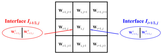
Figure 1.
Diagram of 2D structural grid reconstruction.
When is equal to 1/3, it is the 3rd-order upwind scheme. is the Van Albada limiter [23], which is used to identify smooth/non-smooth areas, and has a small value:
2.2.2. WENO Scheme
The WENO scheme is developed from the ENO scheme. A key idea of WENO is the linear combination of lower order fluxes or reconstruction to obtain a higher order approximation.
where k is the number of stencils, is the nonlinear weighting coefficient, is flux on the different stencil, and is the numerical flux at interface .
At present, the most widely used WENO scheme is the 5th-order WENO-JS [24]. It introduces a parameter characterizing the smoothness of the interpolation function corresponding to the interpolation template—the smoothness factor , which is specifically defined as follows:
where the is cell size.
Based on Equation (13), the nonlinear weighting coefficient can be obtained:
where is a linear weighting factor, and has a small value preventing denominator from being zero, such as . For structural mesh, the finite volume methods have the same format for one and several space dimensions [25].
2.2.3. MP Scheme
The MP scheme can not only maintain the monotonicity of the numerical scheme near the discontinuity point, but also maintain the accuracy near the extreme point, so it is very beneficial to simulate the turbulent flow containing shock waves [26]. The MP interface value is obtained by limiting a high-order polynomial reconstruction, which means this scheme consists of linear interpolation and a nonlinear limiter. The former is used to construct high-precision interpolation, while the latter mainly constrains the monotonicity of the interpolation result at the discontinuity. The linear interpolation function of the 5th-order MP scheme is as follows:
If satisfies the following formula, then it means that the local area is smooth and no limiter is needed.
where the has a small value, and is defined as follows:
Otherwise, the MP limiter needs to be activated to prevent possible non-monotonic interpolation. The 2D/3D reconstruction scheme share the same computing method as 1D.
2.3. Time Integration Scheme
For steady-state calculations, this paper uses the LU-SGS/Runge–Kutta approach for time integration, which can be combined with some acceleration techniques such as using larger CFL numbers and local-time-step integration to quickly reach the steady state. For unsteady-state flow simulations, the Runge–Kutta approach can still be used but dual time-step LU-SGS approach is mainly chosen, which introduces inner iteration on the basis of LU-SGS and the physical time step can be selected according to the actual problem. For all the steady-state simulation in this paper, both large CFL number and the local-time-step integration are applied to accelerate the computation.
2.4. Initial Conditions and Boundary Conditions
When dealing with the initial conditions in this research, the flow parameters about the free stream are usually used to assign initial values for the entire computational domain. However, for some simulations containing extremely complex flow, the initial conditions of the flow field have greater impacts on the subsequent computation results: if the initial values are not appropriate, the calculation can diverge. Therefore, for the high-precision CFD simulation of the supersonic inlet/isolator, the low-order steady-state simulation results can be used as the initial condition. Boundary conditions are a crucial part of CFD computation, and whether they are handled properly has a great impact on the final result. This research mainly involves four types of boundary conditions:
(1) Inlet Boundary Conditions
a. Subsonic: set total temperature, total pressure and flow direction at the entrance;
b. Supersonic: all the parameters are decided by far-field free stream, including density, static pressure and velocity;
(2) Outlet Boundary Conditions
a. Subsonic: set static pressure at the outlet, and the remaining parameters are extrapolated from the inside of the flow field;
b. Supersonic: all the parameters are extrapolated from the inside of the flow field;
(3) No Slip Wall Boundary Condition
For viscous flow, no slip and no penetration conditions are imposed on the wall;
(4) Symmetry Boundary Condition
This boundary condition can be used to reduce computation.
2.5. Mesh
The structural grid is used in this paper, performing local densification where the flow parameter’s gradient changes dramatically. For turbulent flow simulation, the factor near the wall surface is kept equal to 1, and the grid aspect ratio of the mainstream area is roughly ensured to be 1.
2.6. Numerical Test
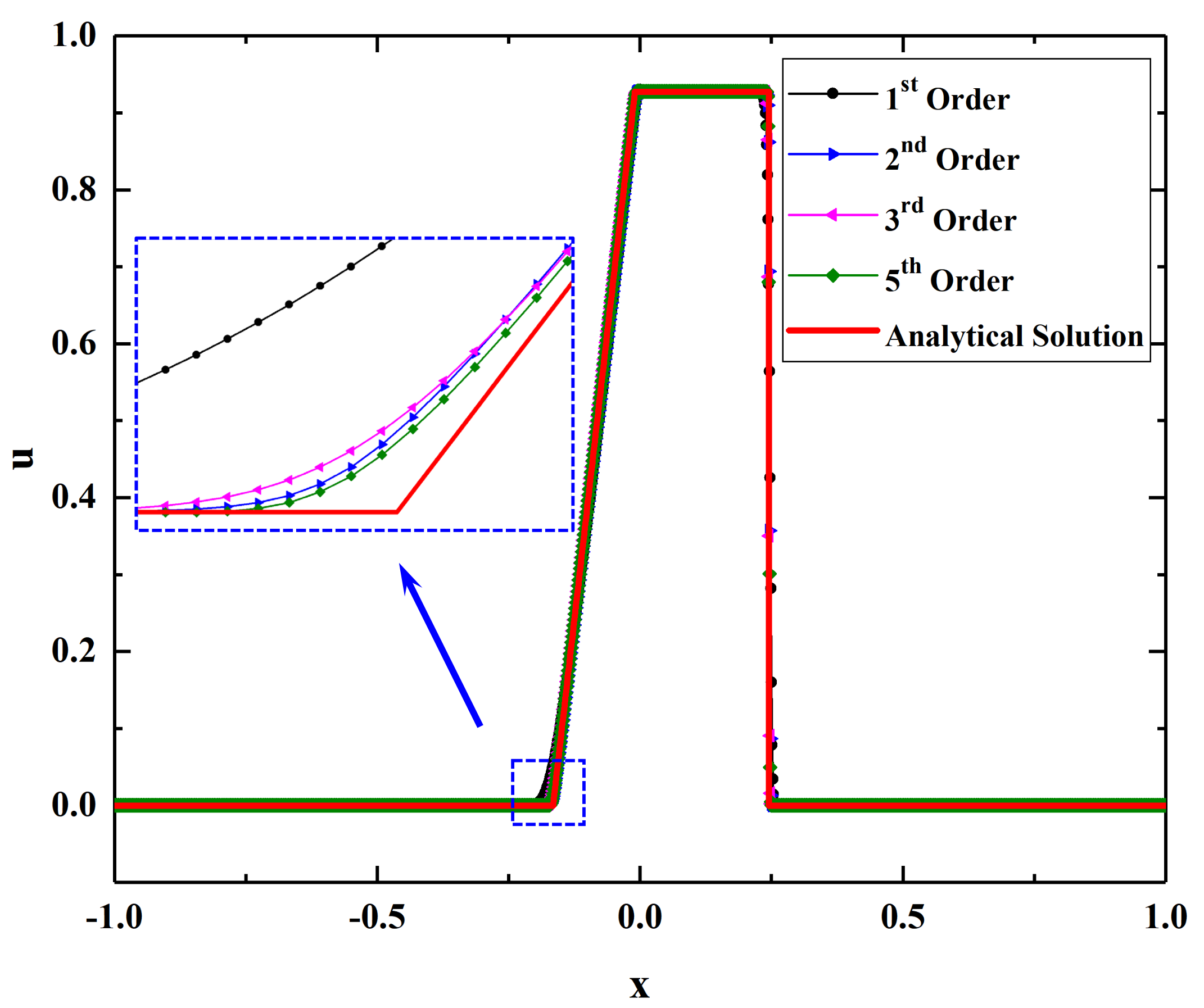
To validate the CFD solver and compare the shock-capturing ability of different reconstruction schemes, the one-dimensional inviscid Sod shock tube problem [27] is adopted here, which is one of the few problems with an analytical solution. The computational domain is [−1,1], and the initial condition is given by:
Figure 2 shows the velocity profiles at time t = 0.14, and all the numerical results are kept consistent with the analytical solution, which also indicates that, the higher the reconstruction order, the better the simulation results will be get.
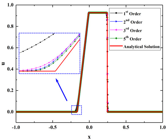
Figure 2.
The velocity profiles of the Sod shock tube problem at time t = 0.14.
3. DES/LES Computation Method
This part of the computation is completed by using the commercial software ANSYS Fluent 18.0, which is briefly introduced below.
3.1. DES Computation
In the field of turbulence simulation, an obvious development trend is toward the hybrid RANS/LES model. In the near-wall area, the RANS method is used to solve the turbulent boundary layer flow state, and the LES method is used in the far-wall area to analyze large-scale vortices. This hybrid approach is an easy-to-implement and representative method [28].
Since the transition zone between the RANS/LES computational domain is prone to exhibiting erroneous behaviors, Spalart proposed the delayed detached eddy simulation (DDES) [29], but both DES and DDES mainly aim to solve complex flow problems with large-scale separation; however, for small separation flow conditions, especially for turbulent flow near the wall, log-layer mismatch always occurs. An improved method is achieved by combining DDES and Wall-Modeled Large Eddy Simulation (WMLES) to propose an improved delayed detached eddy simulation (IDDES) [30], which gives a new definition of the subgrid-length-scale:
where is an empirical constant that is always set equal to 0.15, is the distance to the wall, is the maximum local grid spacing, and is the grid step in the wall-normal direction. Then the length scale of the IDDES model can be constructed:
where and are the length scales for RANS or LES model, respectively, ( depends on Δ). and are both blending functions.
The IDDES model is selected for DES simulation in this research, which is only available for 3D computation. If a 2D flow solution is required, the physical model has to be properly stretched along the thickness direction.
3.2. LES Computation
Compared with the DES computation, LES has a greater computing cost, but it still saves a lot compared with DNS, which also directly avoids the non-universality of the turbulence model under RANS. LES resolves the eddies larger than the filter scale, whose accuracy can reach the inertial range of the turbulent kinetic energy spectrum, and the smaller scale is modeled by establishing a subgrid model, so much more abundant and accurate flow field information can be obtained.
Recently, a variety of subgrid models have been developed. Compared with Wall-Resolved LES (WRLES), Wall-Modeled LES (WMLES) could slightly relax the requirements of the number of grids for computation, but the cost incurs when the turbulence near the wall cannot be resolved. The formula for solving eddy viscosity of WMLES is as follows [30]:
where is an empirical constant equal to 0.2, is equal to 0.41, S is the strain rate, and Δ is the subgrid length-scale, defined as Equation (19).
The WMLES model is used for LES simulation in this research, and since LES is also only available for 3D computation, the same strategy as the DES is adopted.
4. Inlet/Isolator Simulations
4.1. Physical Configuration
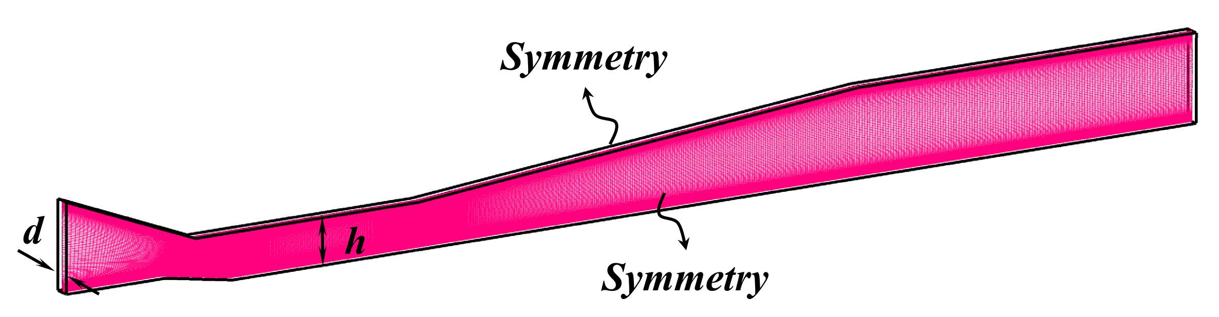
A high-precision numerical simulation of a two-dimensional supersonic inlet/isolator is carried out and compared with experimental data (the data are taken from the hypersonic wind tunnel experimental platform of RWTH Aachen University, Germany) [1]. The detailed geometric parameters of the physical configuration are outlined in Figure 3.
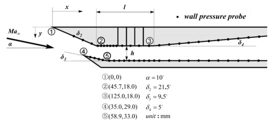
Figure 3.
Configuration of the inlet/isolator: h = 15 mm, l = 79.3 mm.
4.2. Mesh and Boundary Conditions
This paper aims to achieve three different comparisons: 2D RANS computations with different reconstruction schemes, 2D/3D RANS computations, and RANS/DES/LES computations. Therefore, three types of meshes are involved: a 2D structural mesh, a 3D structural mesh and a quasi-3D mesh (for DES and LES computations, the effects of the side wall of the inlet/isolator are not considered here, and the two sides are set as symmetry boundary conditions).
The mesh of the 2D computational domain and the setting of boundary conditions are shown in Figure 4. Here, three sets of multi-block structural meshes with different sparsities are used, as shown in Table 1, which are all refined near the wall. The of the grid’s first layer near the wall is set to 1, and the aspect ratio of the grid in the mainstream area is almost 1. To accelerate the computation, the fluid domain can be divided into many more blocks.
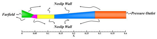
Figure 4.
Mesh of the 2D computational domain.

Table 1.
Three sets of meshes with different sparsities.
The 3D computations must consider the influence of the inlet/isolator’s side wall on the internal flow, which introduces a strong 3D effect. For simplifying the computations, only half of the inlet/isolator is selected by using symmetry boundary condition, as shown in Figure 5.
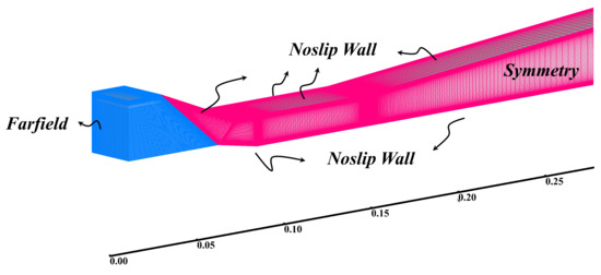
Figure 5.
Mesh of the 3D computational domain.
The quasi-3D computation mesh is the stretching result of the 2D mesh in the thickness direction. To reduce the computation costs as much as possible while ensuring the accuracy of the solution, the stretched thickness d is taken as . From experience, if d were set too small, the computation would diverge, as shown in Figure 6.

Figure 6.
Mesh of the quasi-3D computational domain.
The free stream flow parameters for the farfield conditions are shown in Table 2, and the corresponding turbulent values: turbulent kinetic energy k and specific dissipation rate are determined by the specified turbulent intensity I:
where V is the velocity of the free stream, and is the dynamic viscosity.
Table 2.
Free stream flow parameters: —total Pressure, —total Temperature, I—turbulence intensity.
4.3. Results and Analysis
4.3.1. Results—RANS
(1) 2D Computation
a. Reconstruction: 3rd MUSCL Scheme
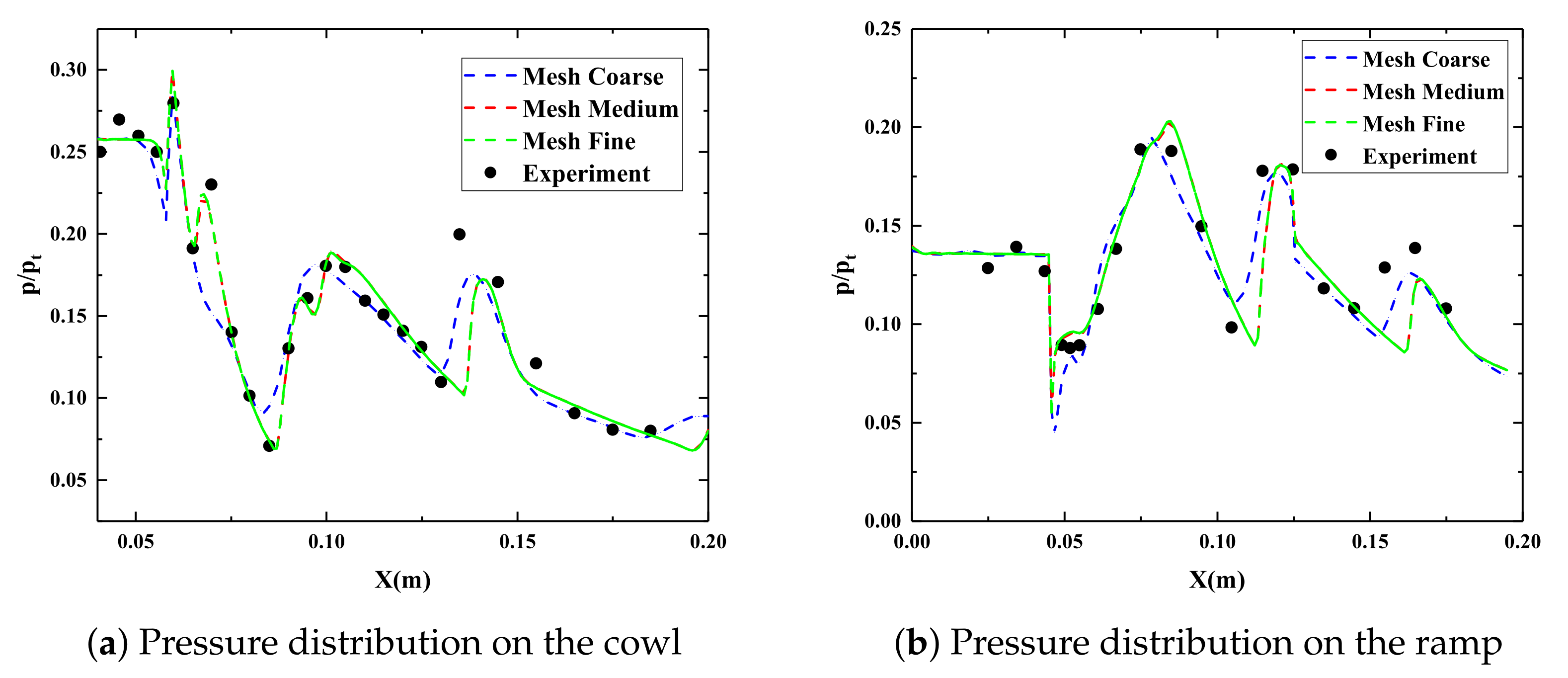
Reinartz [1] mentioned that, for the flow at the central section of the two-dimensional inlet/isolator, the 3D effects of the side wall can be ignored. So, in this part, a 2D simulation based on RANS is performed. In order to complete the grid independence verification, this paper solves three sets of meshes with different sparsity, as mentioned in the last section “Mesh and Boundary Conditions”, by using the compressible RANS-based CFD solver developed: combine the 3rd-order MUSCL reconstruction scheme, the AUSM flux computation scheme, the SST turbulence model and the LU-SGS steady-state time integration approach. The simulation results of different meshes mentioned in Table 1 are shown in Figure 7: all the results are in good agreement with the experimental test, and the simulation outcomes of the medium and fine mesh are almost the same, with only slight differences, so in the subsequent computations, the medium mesh is adopted.
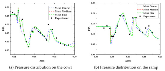
Figure 7.
Comparison of RANS results for three different sparseness meshes.
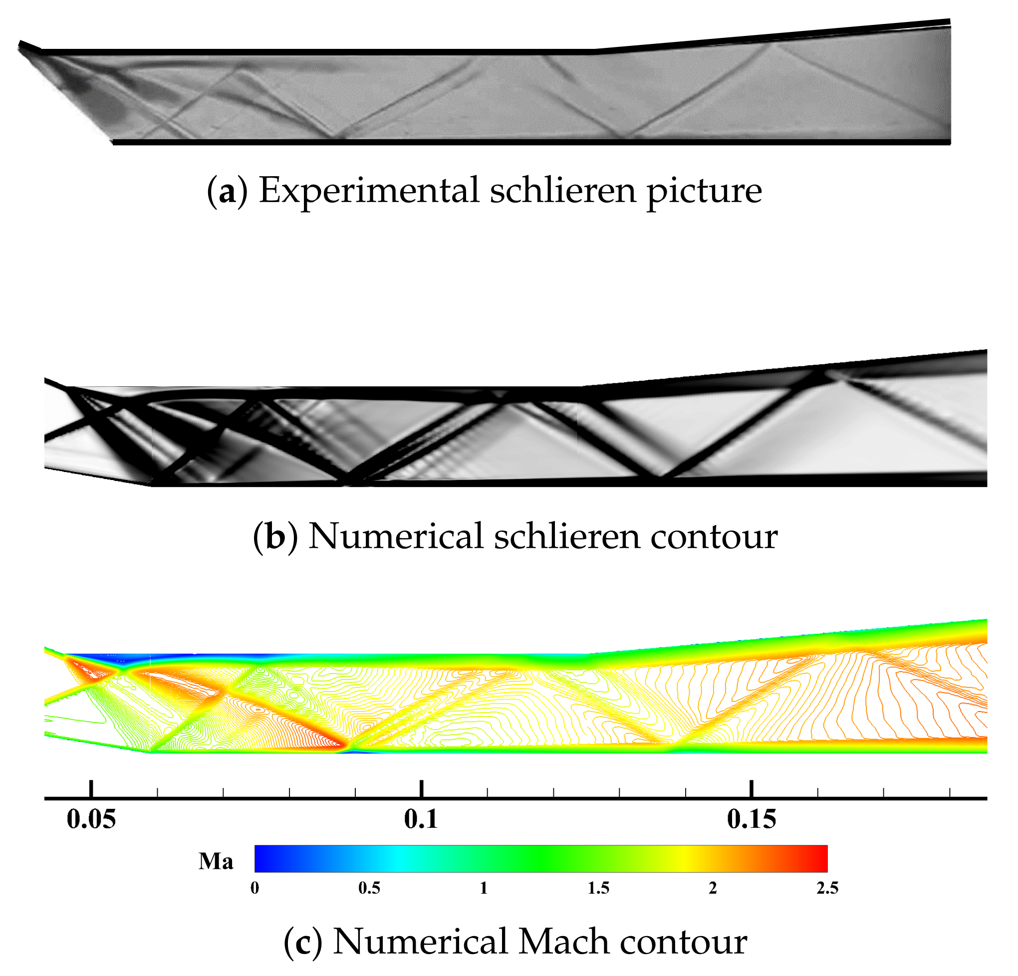
It can be seen from Figure 8 that the wave system inside the intake duct is highly complicated. The oblique shocks are reflected multiple times inside the isolator, and there are strong interactions of shock waves/expansion waves and shock waves/turbulent boundary layers, leading to obvious flow separations near the throat of the inlet. By the comparison of Figure 8, the shocked flow field structure obtained through numerical simulation is basically consistent with the experimental test results, and the pressure distribution is also roughly the same as the test of Figure 7. However, there are some small deviations between them: it can be seen from Figure 7 and Figure 8 that, in the rear part of the isolator, the simulation results show that the oblique shock incident point is slightly farther back, and comparing the experimental Schlieren picture and the computation results, it can be found that the simulation’s boundary layers are thinner and the separation near the throat is smaller.
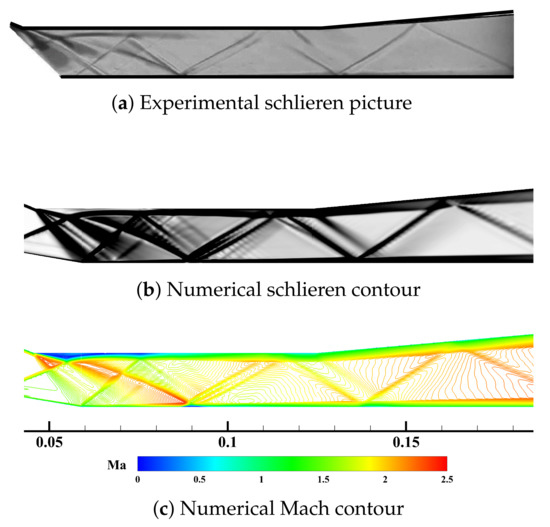
Figure 8.
Comparison of experimental and numerical results.
b. Reconstruction: 5th WENO/MP Scheme
To improve the simulation accuracy, higher order reconstruction schemes are used to obtain the higher flow field resolution. The specific results are shown below.
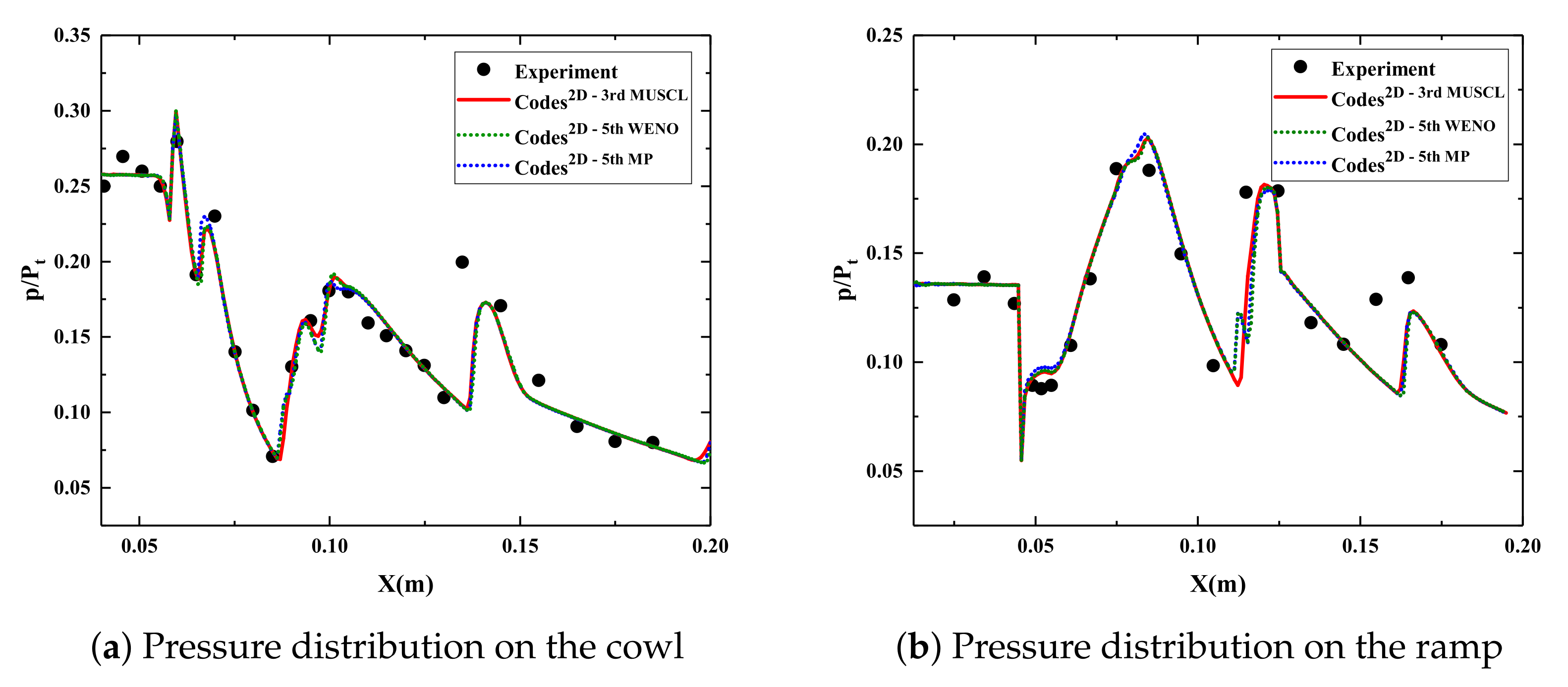
It is obvious in Figure 9 that, for the wall pressure distribution, the higher-order schemes can capture flow field details more accurately, such as is evidenced by the second peak of the pressure at the cowl, and the results of WENO and MP are very similar. Comparing Figure 10 and Figure 8, the separation area obtained by the higher order schemes is more similar to the experimental Schlieren picture. As a result, for a steady-state calculation, the flow fields obtained from the low-order reconstruction schemes can be treated as the initial conditions for the higher order schemes.
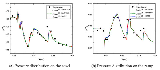
Figure 9.
Comparison of simulation results for the three reconstruction schemes.
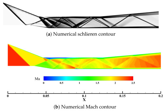
Figure 10.
5th WENO simulation results.
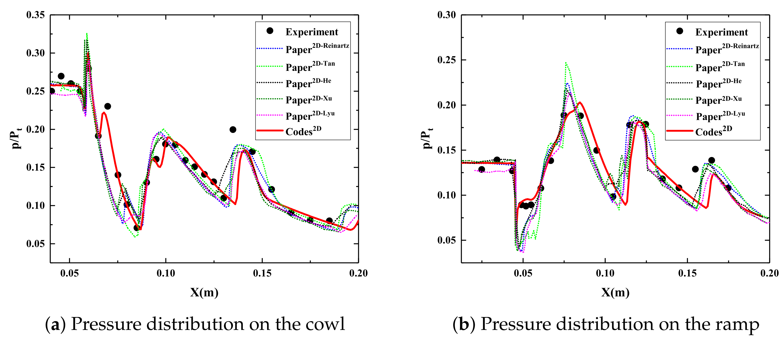
By comparing the results of this paper with those of other research teams [1,7,10,31,32] (most of them are based on ANSYS Fluent, and have partly used in-house CFD solvers), as shown in Figure 11, we verify the computation accuracy of the CFD solver developed in this paper, and also find that the partial deviations between the simulation and experiment are common problems of the 2D RANS computation—the RANS accuracy is limited.
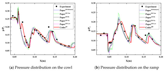
Figure 11.
Comparison of other researchers’ results based on RANS.
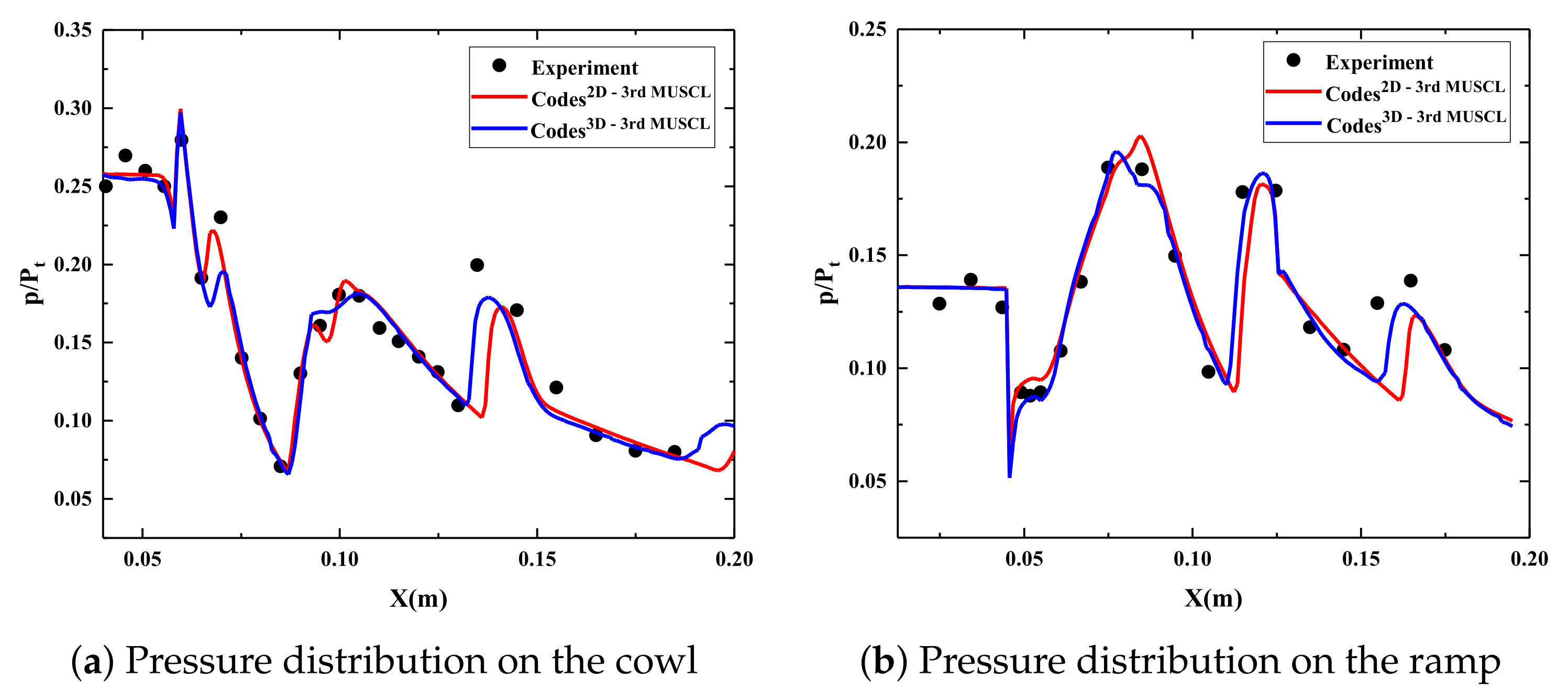
(2) 3D Computation
The 2D computation of the inlet/isolator is a simplified ideal case. In reality, the 3D effects of the side wall may cause unstart under some extreme conditions. Therefore, a 3D computation is performed to compare the 2D/3D simulation results based on RANS. The generation of 3D computation’s mesh is based on the 2D medium mesh, and it is divided into 100 layers in the thickness direction, which are also refined near the side wall, ensuring the of the first layer equals to 1. As shown in Figure 12, there is a strong rolled-up lateral flow near the sidewall of the inlet throat, which also interacts with the separation area at the ramp, and the flow inside the separation bubble is relatively disordered: the flow distribution in the Z direction is extremely uneven, and the 3D effects are quite obvious. Through Figure 13, it can be seen more intuitively that the 3D computation results are closer to the experimental test, which are all extracted from the central plane in Z direction.
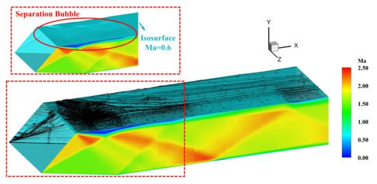
Figure 12.
3D effects of binary supersonic inlet/isolator’s side wall.
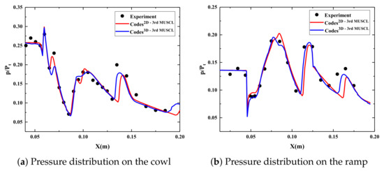
Figure 13.
Comparison of 2D/3D simulation results.
4.3.2. Results—DES/LES
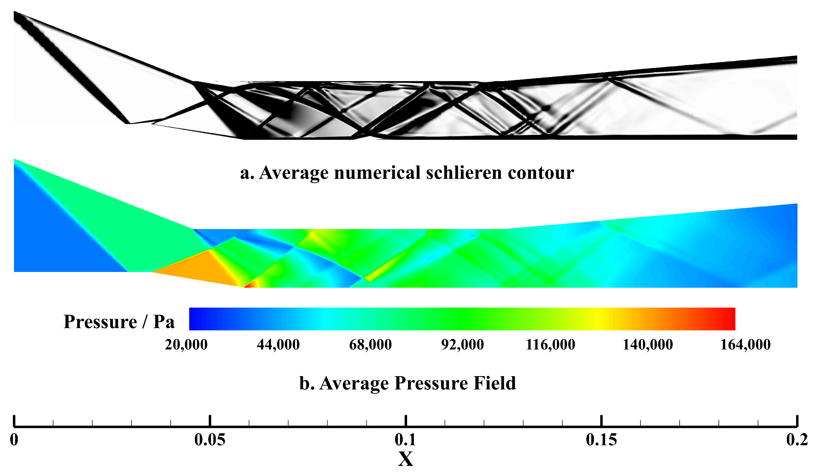
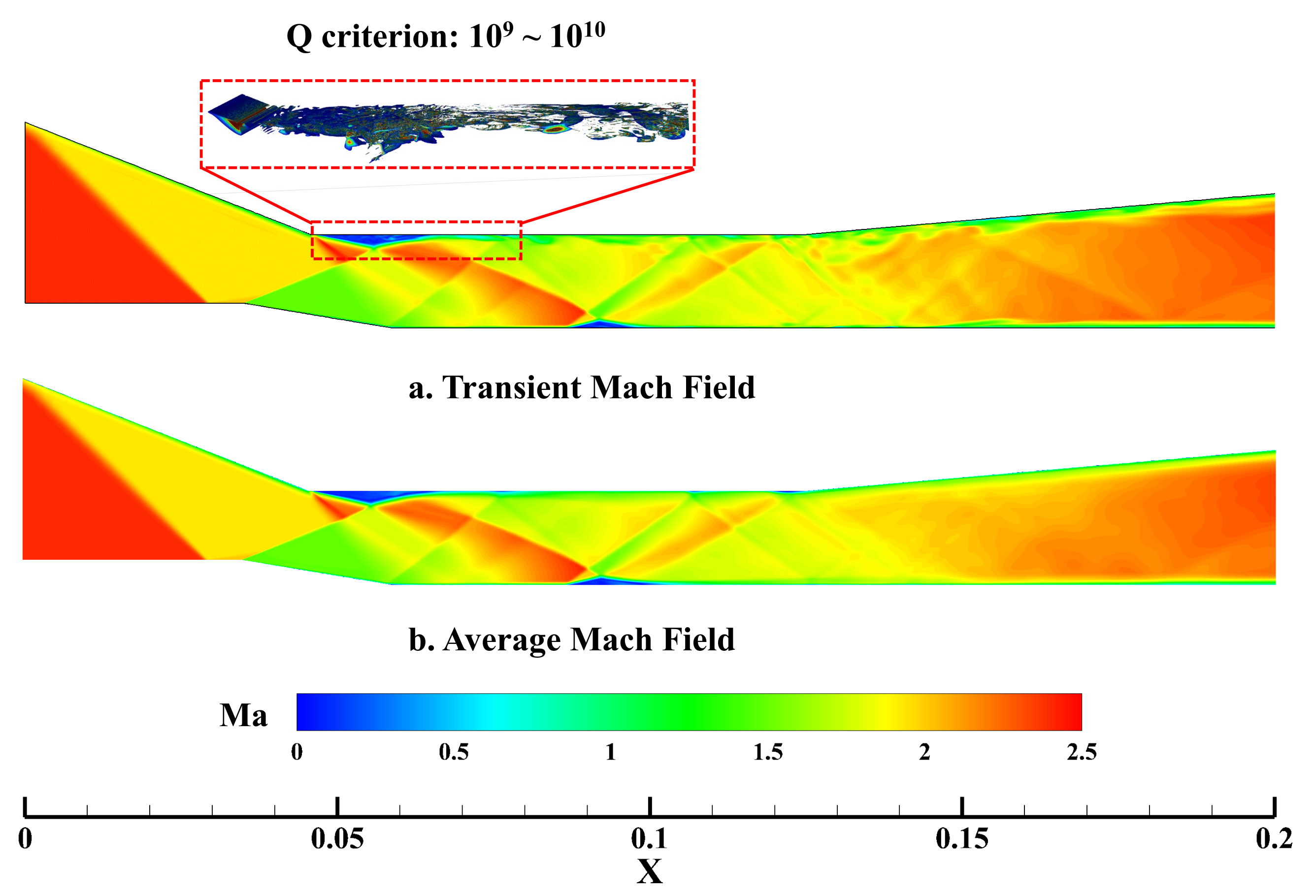
To break through the accuracy restriction of the turbulence model and capture the small vortex structures of the inlet flow, ANSYS Fluent 18.0 is used to perform DES and LES simulations, combined with the second-order upwind reconstruction scheme.The generation of quasi-3D computation’s mesh is based on the 2D fine mesh, which is divided into 50 layers in the thickness direction. The relevant results are shown in Figure 14, Figure 15, Figure 16 and Figure 17.
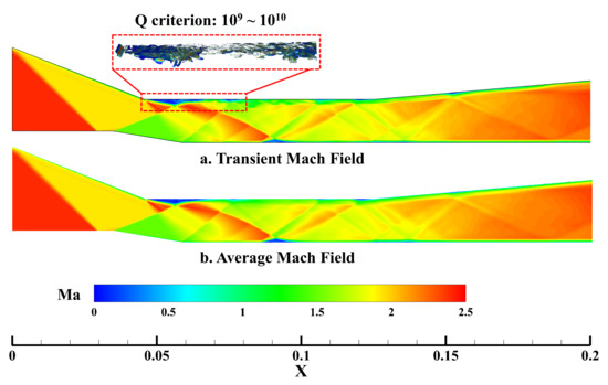
Figure 14.
DES simulation: Mach field.
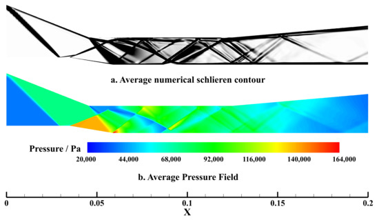
Figure 15.
DES simulation: average fields of density gradient and pressure.

Figure 16.
LES simulation: Mach field.
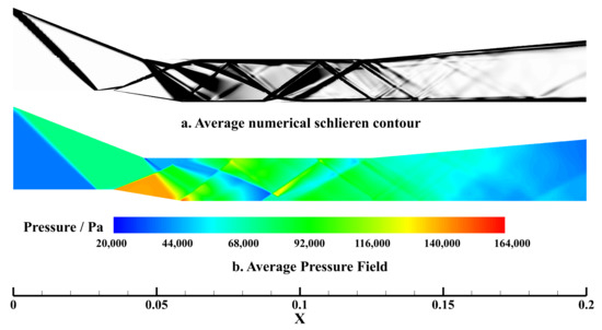
Figure 17.
LES simulation: average fields of density gradient and pressure.
It can be seen from the above contours that DES/LES can capture the vortex structures in the flow on a finer scale. These contours also show that the shock positions inside the inlet/isolator by DES/LES are consistent with the experiment, and the prediction of flow separation area is better than that of RANS. Comparing the time-average Mach fields with those at a certain moment in Figure 14 and Figure 16, it is obvious that there are density fluctuations near the solid walls. This also demonstrates the average pressure fields and the density gradient fields (known as numerical Schlieren contour) of DES/LES simulations. However, due to the low-order reconstruction scheme and limited accuracy of Fluent, it is difficult to extract precise pressure distribution on the cowl/ramp of the inlet/isolator for high flow.
5. Conclusions
This research mainly uses a CFD solver that has been developed based on RANS to perform high-precision and high-efficiency steady-state simulation for the internal flow of a two-dimensional supersonic inlet/isolator, with high order spatial schemes. These findings establish a strong agreement between computational and experimental results, and also show a comparison of the 2D/3D simulation results. Moreover, the commercial software ANSYS Fluent 18.0 was utilized to carry out DES and LES simulations, obtaining the flow field details. In summary, the main conclusions of this research are as follows:
(1) The high-order reconstruction schemes can accurately capture the details of the flow field, which is particularly important for computing the SWTBLI. In this work, by combining the currently widely used turbulence model SST with the 3rd-order MUSCL or the 5th-order WENO/MP reconstruction scheme, the accurate capture of the shocks’ positions inside the inlet/isolator was realized, and the simulation results of the pressure distribution on the cowl/ramp were obtained and were found to be highly consistent with the experiment;
(2) The side wall of the two-dimensional supersonic inlet has a vital impact on the internal airflow conditions, and the 3D effects are obvious. By comparing the pressure distribution on the cowl/ramp obtained by 2D/3D simulations, it can be found that 3D computation can make up for some defects in the 2D results and capture the shocks’ positions and intensities more accurately. Through a detailed analysis of the results of the 3D flow field, it is observed that the side wall of the inlet will induce a strong lateral flow, which interferes with the separation bubbles generated near the throat of the ramp;
(3) The DES and LES computational methods can be used to obtain the flow details near the flow separation area and the boundary layers, but these methods need to be combined with high-order spatial discretization schemes. Otherwise, they cannot accurately capture the vortex structures in the complex flow, leading to certain deviations between the computational and experimental results.
Author Contributions
Investigation, Z.L.; methodology, Z.L. and Z.X.; software, Z.L.; formal analysis, Z.L. and Z.Z.; data curation, Z.L.; visualization, Z.L., C.W. and K.Z.; writing—original draft, Z.L., Z.X. and C.W.; writing—review & editing, Z.L., C.W., K.Z., Z.Z. and Z.X.; resources, Z.X.; conceptualization, Z.X.; supervision, Z.X. All authors have read and agreed to the published version of the manuscript.
Funding
This research received no external funding.
Acknowledgments
Thanks are due to Yufei Zhang, Jingyuan Wang and Dongdong Zhong of Tsinghua University for valuable discussion.
Conflicts of Interest
The authors declare no conflict of interest.
References
- Reinartz, B.U.; Herrmann, C.D.; Ballmann, J.; Koschel, W.W. Aerodynamic performance analysis of a hypersonic inlet isolator using computation and experiment. J. Propuls. Power 2003, 19, 868–875. [Google Scholar] [CrossRef]
- Herrmann, D.; Gülhan, A. Experimental analyses of inlet characteristics of an airbreathing missile with boundary-layer bleed. J. Propuls. Power 2015, 31, 170–179. [Google Scholar] [CrossRef]
- Anderson, W.E.; Wong, N.D. Experimental Investigation of a Large Scale, Two-Dimensional, Mixed-Compression Inlet System-Performance at Design Conditions, M = 3.0; NASA Ames Research Center Moffett Field: Mountain View, CA, USA, 1970. [Google Scholar]
- Emami, S.; Trexler, C.A.; Auslender, A.H.; Weidner, J.P. Experimental Investigation of Inlet-Combustor Isolators for a Dual-Mode Scramjet at a Mach Number of 4; NASA: Hampton, VA, USA, 1995. [Google Scholar]
- Huang, H.; Tan, H.; Zhuang, Y.; Sheng, F.; Sun, S. Progress in Internal Flow Characteristics of Hypersonic Inlet/Isolator. J. Propuls. Technol. 2018, 39, 2252–2273. [Google Scholar]
- Rumsey, C.; Smith, B.; Huang, G. Description of a website resource for turbulence modeling verification and validation. In Proceedings of the 40th Fluid Dynamics Conference and Exhibit, Chicago, IL, USA, 28 June–1 July 2010; p. 4742. [Google Scholar]
- Xu, K.; Chang, J.; Zhou, W.; Yu, D. Mechanism and prediction for occurrence of shock-train sharp forward movement. AIAA J. 2016, 54, 1403–1412. [Google Scholar] [CrossRef]
- Li, N.; Chang, J.; Yu, D.; Bao, W.; Song, Y. Mathematical model of shock-train path with complex background waves. J. Propuls. Power 2017, 33, 468–478. [Google Scholar] [CrossRef]
- Reardon, J.P.; Schetz, J.A.; Lowe, K.T. Computational Analysis of Unstart in Variable-Geometry Inlet. J. Propuls. Power 2021, 1–13. [Google Scholar] [CrossRef]
- He, Y.; Huang, H.; Yu, D. Investigation of boundary-layer ejecting for resistance to back pressure in an isolator. Aerosp. Sci. Technol. 2016, 56, 1–13. [Google Scholar] [CrossRef]
- Morgan, B.; Duraisamy, K.; Lele, S.K. Large-eddy simulations of a normal shock train in a constant-area isolator. AIAA J. 2014, 52, 539–558. [Google Scholar] [CrossRef]
- Koo, H.; Raman, V. Large-eddy simulation of a supersonic inlet-isolator. AIAA J. 2012, 50, 1596–1613. [Google Scholar] [CrossRef]
- Slotnick, J.P.; Khodadoust, A.; Alonso, J.; Darmofal, D.; Gropp, W.; Lurie, E.; Mavriplis, D.J. CFD Vision 2030 Study: A Path to Revolutionary Computational Aerosciences. 2014. Available online: https://ntrs.nasa.gov/citations/20140003093 (accessed on 5 October 2021).
- Spalart, P.R.; Rumsey, C.L. Effective inflow conditions for turbulence models in aerodynamic calculations. AIAA J. 2007, 45, 2544–2553. [Google Scholar] [CrossRef]
- Wilcox, D.C. Formulation of the kw turbulence model revisited. AIAA J. 2008, 46, 2823–2838. [Google Scholar] [CrossRef] [Green Version]
- Chien, K.Y. Predictions of channel and boundary-layer flows with a low-Reynolds-number turbulence model. AIAA J. 1982, 20, 33–38. [Google Scholar] [CrossRef]
- Menter, F.R.; Kuntz, M.; Langtry, R. Ten years of industrial experience with the SST turbulence model. Turbul. Heat Mass Transf. 2003, 4, 625–632. [Google Scholar]
- Knight, D. Elements of Numerical Methods for Compressible Flows; Cambridge University Press: Cambridge, UK, 2006; Volume 19. [Google Scholar]
- Blazek, J. Computational Fluid Dynamics: Principles and Applications; Butterworth-Heinemann: Oxford, UK, 2015. [Google Scholar]
- LII, W.S. The viscosity of gases and molecular force. Lond. Edinb. Dublin Philos. Mag. J. Sci. 1893, 36, 507–531. [Google Scholar]
- Roe, P.L. Approximate Riemann solvers, parameter vectors, and difference schemes. J. Comput. Phys. 1981, 43, 357–372. [Google Scholar] [CrossRef]
- Liou, M.S. A sequel to ausm: Ausm+. J. Comput. Phys. 1996, 129, 364–382. [Google Scholar] [CrossRef]
- Van Albada, G.D.; Van Leer, B.; Roberts, W. A comparative study of computational methods in cosmic gas dynamics. In Upwind and High-Resolution Schemes; Springer: Berlin/Heidelberg, Germany, 1997; pp. 95–103. [Google Scholar]
- Cockburn, B.; Johnson, C.; Shu, C.W.; Tadmor, E. Advanced Numerical Approximation of Nonlinear Hyperbolic Equations. In Proceedings of the 2nd Session of the Centro Internazionale Matematico Estivo (CIME), Cetraro, Italy, 23–28 June 1997; Springer: Berlin/Heidelberg, Germany, 2006. [Google Scholar]
- Shu, C.W. High-order finite difference and finite volume WENO schemes and discontinuous Galerkin methods for CFD. Int. J. Comput. Fluid Dyn. 2003, 17, 107–118. [Google Scholar] [CrossRef]
- Cui, J.; Fang, J.; Yuan, J.; Lu, L. Assessment of monotonicity-preserving scheme for large-scale simulation of turbulence. J. Beijing Univ. Aeronaut. Astronaut. 2013, 39, 488–493. [Google Scholar]
- Sod, G.A. A survey of several finite difference methods for systems of nonlinear hyperbolic conservation laws. J. Comput. Phys. 1978, 27, 1–31. [Google Scholar] [CrossRef] [Green Version]
- Fröhlich, J.; Von Terzi, D. Hybrid LES/RANS methods for the simulation of turbulent flows. Prog. Aerosp. Sci. 2008, 44, 349–377. [Google Scholar] [CrossRef]
- Spalart, P.R.; Deck, S.; Shur, M.L.; Squires, K.D.; Strelets, M.K.; Travin, A. A new version of detached-eddy simulation, resistant to ambiguous grid densities. Theor. Comput. Fluid Dyn. 2006, 20, 181–195. [Google Scholar] [CrossRef]
- Shur, M.L.; Spalart, P.R.; Strelets, M.K.; Travin, A.K. A hybrid RANS-LES approach with delayed-DES and wall-modelled LES capabilities. Int. J. Heat Fluid Flow 2008, 29, 1638–1649. [Google Scholar] [CrossRef]
- Hang, Z.; Huijun, T.; Shu, S. Characteristics of shock-train in a straight isolator with interference of incident shock waves and corner expansion waves. Acta Aeronaut. Astronaut. Sin. 2010, 31, 1733–1739. [Google Scholar]
- Lyu, G.; Gao, Z.; Qian, Z.; Jiang, C.; Lee, C.H. Studies on unsteady mode transition of a turbine based combined cycle (TBCC) inlet with multiple movable panels. Aerosp. Sci. Technol. 2021, 111, 106546. [Google Scholar] [CrossRef]


Publisher’s Note: MDPI stays neutral with regard to jurisdictional claims in published maps and institutional affiliations. |
© 2021 by the authors. Licensee MDPI, Basel, Switzerland. This article is an open access article distributed under the terms and conditions of the Creative Commons Attribution (CC BY) license (https://creativecommons.org/licenses/by/4.0/).