Abstract
Potash seams are a valuable resource containing several economically interesting, but also highly soluble minerals. In the presence of water, uncontrolled leaching can occur, endangering subsurface mining operations. In the present study, the influence of insoluble inclusions and intersecting layers on leaching zone evolution was examined by means of a reactive transport model. For that purpose, a scenario analysis was carried out, considering different rock distributions within a carnallite-bearing potash seam. The results show that reaction-dominated systems are not affected by heterogeneities at all, whereas transport-dominated systems exhibit a faster advance in homogeneous rock compositions. In return, the ratio of permeated rock in vertical direction is higher in heterogeneous systems. Literature data indicate that most natural potash systems are transport-dominated. Accordingly, insoluble inclusions and intersecting layers can usually be seen as beneficial with regard to reducing hazard potential as long as the mechanical stability of leaching zones is maintained. Thereby, the distribution of insoluble areas is of minor impact unless an inclined, intersecting layer occurs that accelerates leaching zone growth in one direction. Moreover, it is found that the saturation dependency of dissolution rates increases the growth rate in the long term, and therefore must be considered in risk assessments.
1. Introduction
The role of potash seams within salt deposits can be viewed from different perspectives: on the one hand, they are a valuable resource that has been mined for many decades; on the other hand, they represent potential risks for technical caverns and subsurface waste repositories [1]. However, both perspectives consider the uncontrolled leaching of potash seams as highly critical. Whether water contact is enabled by geological fault zones or mining activities: in both cases, the increased solubility of potash salt causes a preferential expansion of leaching zones, jeopardizing the integrity and mechanical stability of mines or technical caverns [2,3,4,5]. In order to assess the hazard potential of leaching zones in potash seams, their evolution has to be described in space and time.
Steding et al. [6] developed a reactive transport model complemented by the “interchange approach” to reproduce the complex interplay between chemical reactions and density-driven transport of species within potash seams. The authors showed that leaching zones can be classified into four different groups based on the Péclet (Pe) and Damköhler (Da) numbers, which indicate if a system is dominated by reactions (Da < 1) or transport (Da > 1), and if species transport is dominated by diffusion (Pe < 2) or advection (Pe > 2). However, only homogeneous potash seams have been investigated thus far. Studies on technical cavern construction in rock salt reveal that inclusions or intersecting layers of insoluble materials, such as mudstone, gypsum or sandstone, lead to highly irregular cavern shapes [7,8,9]. Furthermore, inclined layers can cause an asymmetric expansion of leaching zones [10]. To investigate if similar phenomena occur within potash seams, heterogeneous rock distributions need to be examined. In addition, mineralogical heterogeneity and the associated variations in dissolution rate need to be taken into account, because these can significantly influence dissolution structure, especially at high Péclet numbers [11,12].
For this purpose, the reactive transport model presented by Steding et al. [6] was extended by mineral-specific, saturation-dependent dissolution rates, and a scenario analysis under density-driven flow conditions was performed. Thereby, six generic mineral distributions were investigated, with insoluble areas ranging from several small inclusions to one continuous layer. The main objective was to determine the influence of insoluble layers and inclusions on the evolution and hazard potential of leaching zones within potash seams, and if a risk assessment based on the Pe and Da numbers is still feasible.
2. Materials and Methods
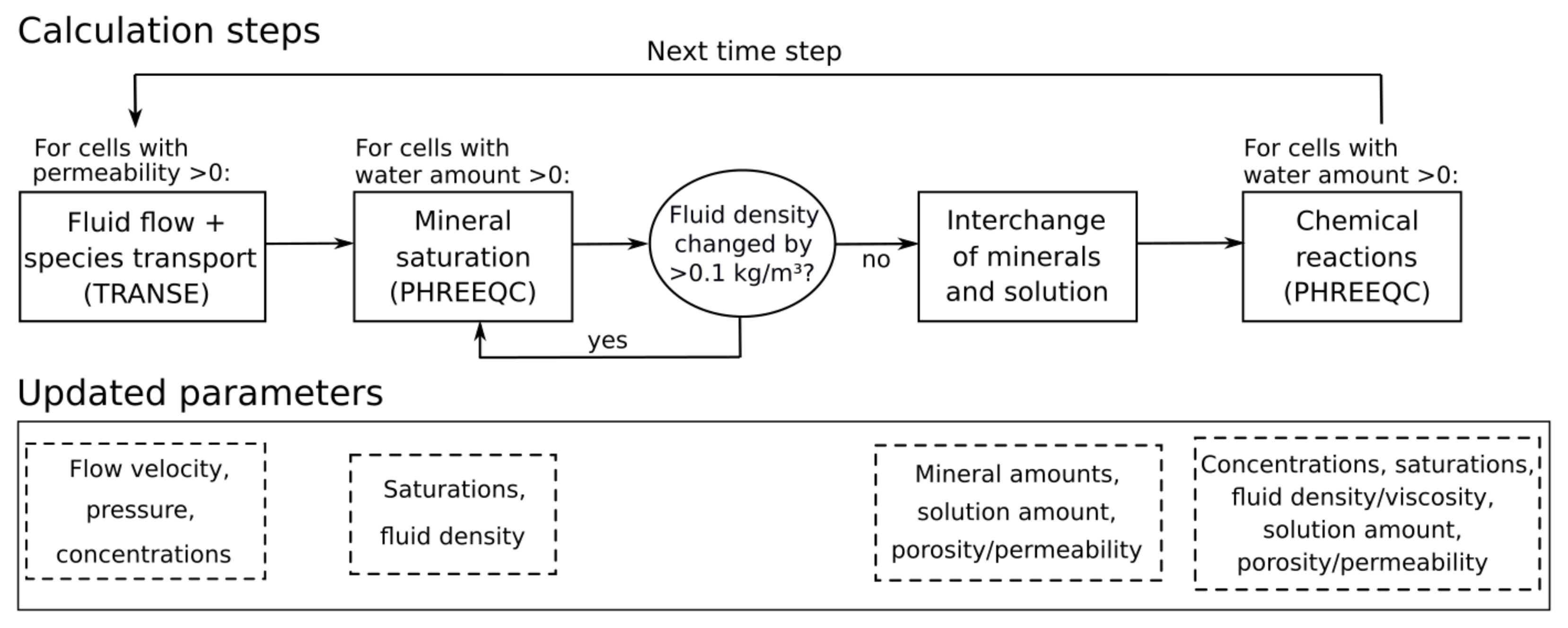
The concept of the applied reactive transport model is shown in Figure 1. Each simulation time step starts with the solution of the partial differential equations for the fluid flow and transport of chemical species using the TRANsport Simulation Environment (TRANSE) [13]. TRANSE is coupled with the geochemical reaction module PHREEQC [14], applied in combination with the THEREDA database [15]. In the second calculation step, PHREEQC is used to update fluid densities and mineral saturations following transport. After that, the “interchange” step is performed, which describes the dissolution of minerals from (nearly) dry into permeated cells and allows the dissolution front to progress [6]. The terms “dry” and “permeated” are used in view of the fluid saturation in the pore space, whereas the term “saturated” refers to the chemical equilibration of the solution with respect to salt minerals. In the final calculation step, the chemical reactions resulting from transport and interchange are determined using PHREEQC. Thereby, thermodynamic equilibrium is assumed within each cell. The updated concentrations and fluid properties, such as density and viscosity, are then transferred back to TRANSE to calculate flow and transport in the next simulation time step (Figure 1). More details on this procedure are presented in Steding et al. [6]. The interchange of minerals and solution has been extended in the present study and will be described in detail in the following subsection.
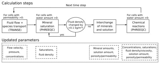
Figure 1.
Flow sheet of the coupled reactive transport model: calculations undertaken at each simulation time step and associated output parameters (modified from Steding et al. [6]).
2.1. Extended Interchange Approach
In Steding et al. [6], constant dissolution rates were used to calculate the interchange of salt minerals. However, it is known that close to equilibrium, the dissolution rates decrease considerably [16,17,18]. Based on the results of Alkattan et al. [19], a linear saturation dependency is assumed:
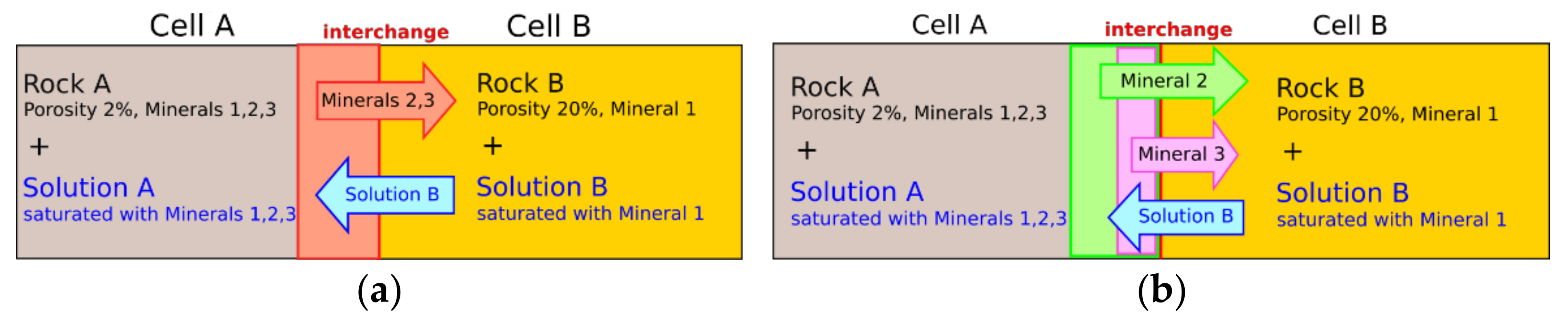
where kmax (cm/s) is the dissolution rate in an infinitely dilute solution. Q is the activity product and K the equilibrium constant. The saturation index SI (-) results from log(Q/K). Leaching zones can contain several primary and secondary minerals that differ in maximum dissolution rate kmax as well as in saturation state [20]; therefore, an average dissolution rate for the potash seam (Figure 2a) is not applicable here. Instead, the dissolution rate according to Equation (1) and the amount of minerals dissolved into an adjacent cell Minsol (mol) need to be calculated individually for each mineral (Figure 2b). Thereby, rate (cm/s) always refers to the saturation state of the solution into which the mineral is dissolved. Between Cell A and Cell B, the amount of interchanged mineral n can be calculated with Equation (2):
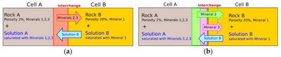
Figure 2.
Sketch of the interchange approach with (a) constant and (b) variable dissolution rates. A defined amount of each mineral according to Equation (2) is dissolved from a cell with low porosity (Cell A) into an adjacent cell with higher porosity (Cell B). These amounts are cumulated, and the solution is transferred into the cell with lower porosity to fill the newly formed pore space (modified from Steding et al. [6]).
The amount of mineral n present in Cell A, MinA,n (mol), divided by the cell diameter perpendicular to the dissolution front di (cm), gives the affected amount of mineral n if the width of 1 cm is dissolved from Cell A. To take into account the contact area between the rock in Cell A and the solution in Cell B, this amount is multiplied with the porosity difference between both cells (ΦB−ΦA) and divided by the volume fraction of the rock in Cell A (1−ΦA). If ΦA ≥ ΦB, the interchange is zero, i.e., minerals can only be dissolved into adjacent cells with higher porosity. dt (s) is the length of the simulation time step. If the solution in Cell B is already saturated with respect to n, raten becomes zero and the mineral is not dissolved. The interchange takes place at each interface between two cells within the model. The volumes of all minerals dissolved at one interface are cumulated to determine the amount of solution that is transferred in return to keep the volume of both cells constant (Figure 2).
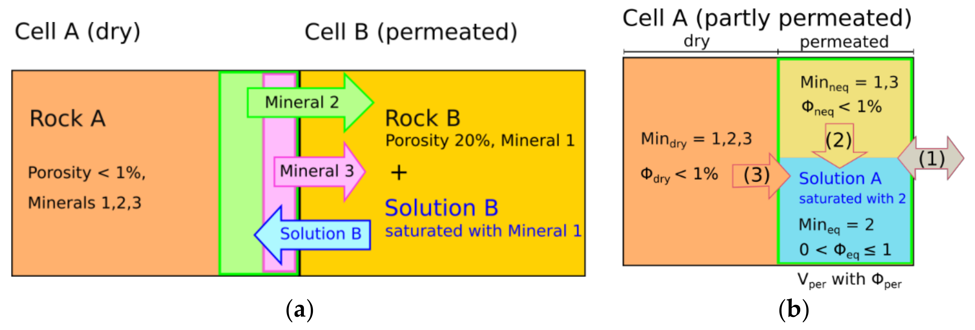
At the dissolution front, the interchange approach enables originally dry cells to receive solution for the first time from an adjacent cell (Figure 3a). The solution needs to be undersaturated with at least one of the minerals from the dry rock; otherwise, no interchange takes place. Newly permeated cells are divided into a permeated and a dry sub-cell to avoid immediate drying out due to high solid-fluid-ratios (Figure 3b). In cases of constant dissolution rates, all minerals in the permeated part were assumed to be in equilibrium with the solution of the cell, whereas minerals in the dry part were not considered in the subsequent calculation of chemical reactions [6]. However, as shown in Figure 3a, the varying dissolution rates challenge the identification of a clear borderline between dry and permeated or equilibrated and non-equilibrated parts, respectively. It can be seen that Mineral 2 has the highest dissolution rate, and therefore limits the region of increased porosity where mineral solution occurs (green). Within this region, it is reasonable to equilibrate the solution with regard to Mineral 2. However, Mineral 3 has a lower dissolution rate, and can therefore only be equilibrated with the solution in the pink subregion. Following this reasoning, one would end up with an additional subregion for each mineral, which is of course not practical. Instead, the permeated part within each cell is split up into minerals that are in equilibrium with the solution (equilibrated minerals Mineq) and such that are not (non-equilibrated minerals Minneq; Figure 3b). Thereby, the volume of the permeated part Vper is determined by the most soluble mineral (Mineral 2, green area). Outside of this area, the salt rock is still dry and the composition Mindry corresponds to the originally unaffected potash seam. In contrast, minerals within the permeated area Vper are surrounded by solution, whereby it is not yet in equilibrium with all minerals. Minerals that remain undissolved during the interchange due to their lower dissolution rates (Mineral 1 and parts of Mineral 3 within the green area, Figure 3a) are assigned to the non-equilibrated minerals Minneq. In contrast, precipitations from Solution B belong to the minerals equilibrated with the solution Mineq.
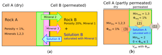
Figure 3.
Sketch of the interchange at the dissolution front (a) resulting in a partly permeated cell (b). The permeated part Vper contains minerals Mineq that are in equilibrium with Solution A and minerals Minneq that are not. In addition to interchange with adjacent Cells (1), the internal dissolution of non-equilibrated Minerals (2) and dry Minerals (3) is considered following Equations 2,4,5, (modified from Steding et al. [6]).
In the case of partly permeated cells, three different types of dissolution can occur (Figure 3b): the first one is interchange with the (fully permeated) adjacent cells according to Equation (2). For this, all three mineral compositions Mindry, Mineq and Minneq, are added together to determine MinA. ΦA is the average porosity of the cell calculated from the volume of MinA related to the cell volume. If the partly permeated cell shows a higher average porosity than the fully permeated one, the interchange of minerals is possible in the reverse direction as well. The dissolved amount of each mineral is split among Mindry, Mineq and Minneq, according to their contribution to the total amount of this mineral. The solution transferred in return is mixed with the pre-existing solution in the permeated part. The chemical reactions resulting from the mixing and the following equilibration with Mineq are determined after the interchange (Figure 1).
In addition to the interchange, internal dissolution processes within cells containing dry (Mindry) or non-equilibrated (Minneq) minerals need to be taken into account (Figure 3b). The interface area between a dry part and the adjacent permeated part(s) is assumed to be constant over time. At the beginning, when the cell is completely dry, the adjacent permeated area is the neighbor cell and dry minerals can only be dissolved via interchange. Accordingly, the interface area is the interface between both cells, which is the cell width multiplied by its height. As Vper increases, Mindry makes up a smaller part of the total mineral amount within the partly permeated cell and its interchange amount decreases. At the same time, the interface area between the dry and permeated parts within the partly permeated cell increases, enhancing the internal dissolution of dry minerals. To account for that, the permeation state of the cell Sper (-) is calculated referring to the volume of the permeated part Vper in relation to the cell volume Vcell:
The higher the Sper, the more the dry rock is dissolved into the solution of its own cell (by internal dissolution) instead of the adjacent cell (by interchange). Equation (4) is used to determine the amount of mineral n dissolved from Mindry into the solution within the permeated part:
Generally, Equation (4) is identical to Equation (2), but multiplied by the permeation state Sper. rate is calculated from the saturation state within the partly permeated cell using Equation (1). In order to determine the affected amount of mineral n if a width of 1 cm of the dry part is dissolved, the present amount, Mindry,n (mol), is divided by the diameter of the dry part perpendicular to the dissolution front. Therefore, the cell diameter di (cm) is now multiplied by the volume ratio of the dry part (1–Sper). The porosity within the dry part is nearly zero, simplifying the term (ΦB–ΦA)/(1–ΦA) in Equation (2) to ΦB, which equals the average porosity of the permeated part Φper. The dissolved amount of each mineral Minsol,dry is added to Mineq. The same applies to precipitations resulting from the equilibration after the interchange (Figure 1). Similar to the interchange of dry minerals, the highest dissolution rate according to Equation (1) determines the volume that is newly added to the permeated part Vper (Figure 3). For minerals with lower dissolution rates, the difference between the amount within this volume and the dissolved amount is added to Minneq.
Finally, the internal dissolution of non-equilibrated minerals (Minneq) has to be taken into account (Figure 3b). These minerals belong to the permeated part of a cell and are already surrounded by solution. However, when the area is permeated for the first time, their dissolution rate is too low to dissolve all minerals. Basically, there are two possible reasons for this: either the maximum dissolution rate kmax is (much) lower than that of the other minerals, or the solution is already (nearly) saturated with these. In the latter case, one could add them to Mineq without changing the solution or rock composition of the permeated part. However, the solution composition changes over time, and originally saturated minerals may become undersaturated. In this case, an immediate equilibration could induce errors because the lower dissolution rates would be neglected. To account for the variation of dissolution rates, Minneq is added stepwise to the solution. The dissolved amount Minsol,neq (mol) of each mineral is determined by Equation (5):
The rate law is similar to those used for interchange (Equation (2)) and the internal dissolution of dry minerals (Equation (4)). Again, rate (cm/s) is calculated from the saturation state within the partly permeated cell according to Equation (1). Minneq (mol) divided by the volume of the non-equilibrated minerals Vneq (cm3) and multiplied by the contact area between non-equilibrated minerals and solution (cm2) gives the amount of mineral n if a width of 1 cm of the non-equilibrated minerals is dissolved. Vneq is calculated from the mineral amounts and densities in Minneq, neglecting small porosities. However, the contact area between non-equilibrated minerals and solution is hard to determine, because the pore structure and spatial arrangement of the different minerals in the original rock are unknown. Therefore, a variable called factor (-) is introduced. If it is set to 1, a rectangular contact area similar to that between Mindry and the solution (Equation (4)) is assumed. This can be seen as a minimum value. If precipitations do not block the access to Minneq, the contact area to the solution flowing between the non-equilibrated minerals should be several times higher. Therefore, it can make sense to simplify the approach and to directly add Minneq to Mineq. In this case, it is assumed that the contact area is large enough to immediately equilibrate minerals and solution within an originally dry volume as soon as the first mineral has been dissolved from it. However, this is only realistic if the maximum mineral dissolution rates do not vary by several orders of magnitude. Furthermore, the first mineral dissolved should make up more than a few vol.% of the dry rock in order to create a sufficiently large contact area. If this is not the case, the internal dissolution of non-equilibrated minerals has to be considered. For some minerals, this may take much longer than the permeation of the cell, i.e., fully permeated cells can still contain non-equilibrated minerals (Figure 4). For the interchange according to Equation (2), Mineq and Minneq are added up to determine MinA and ΦA is defined as the average porosity of equilibrated and non-equilibrated areas.
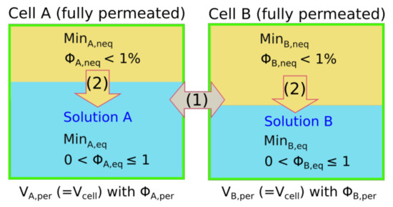
Figure 4.
Fully permeated cells can still contain non-equilibrated minerals due to their lower dissolution rates. Internal dissolution (2) within a cell reduces the amount of non-equilibrated minerals; additionally, they are considered for Interchange (1). The average porosity of the permeated part Φper corresponds to the average porosity of the cell and is used for interchange as well as for flow and transport calculations.
Generally, it is assumed that minerals belonging to Mineq are first dissolved if an undersaturation occurs. As a result, the interchange or internal dissolution of minerals present in Mineq is not possible. Chemical reactions resulting from the processes described above are determined in the final calculation step of the simulation (Figure 1). Thereby, thermodynamic equilibrium is assumed in every cell. The average porosity of the cell is always used in the flow and transport simulation step.
2.2. Scenario Analysis
In order to study the influence of heterogeneities, leaching processes in a carnallite-bearing potash seam containing insoluble layers or inclusions were simulated. Carnallitite is a very common, globally occurring potash salt whose leaching behavior was studied for homogeneous rock compositions by Steding et al. [6]. It was found that transport- and advection-dominated systems (Da > 1 and Pe > 2) are most common and also most critical in the short term with regard to hazard potentials, whereas reaction- and advection-dominated systems (Da < 1 and Pe > 2) become more critical in the long term. Both cases were investigated in this study to identify possible differences in the effect of heterogeneities.
According to Steding et al. [6], 25 wt.% carnallite is a sufficiently high ratio to produce Pe > 2 and low enough to ensure that Darcy flow is still maintained. Therefore, a carnallite-bearing potash seam composition of 25 wt.% carnallite (KMgCl3∙6H2O), 72 wt.% halite (NaCl) and 3 wt.% sylvite (KCl) was applied in all scenarios, corresponding to the volume fractions shown in Figure 5. Mineral densities and dissolution properties are provided in Table 1. The dissolution rate kmax strongly depends on the hydrodynamic boundary conditions: it increases with flow velocity [21] and reaches values under turbulent flow conditions that are at least one order of magnitude higher than that for laminar flow [16,19]. This is due to most salt minerals showing transport-controlled dissolution behavior, i.e., kmax is controlled by the thickness of the diffusive boundary layer at the mineral surface [19,22,23]. The boundary layer thickness, and consequently kmax, depend on the flow velocity, diffusion coefficients and surface roughness [24,25,26,27]. Based on the values of Röhr [17], an average kmax of 5 × 10⁻⁴ cm/s was applied to all three minerals in Table 1. However, this is an upper value because it refers to convection in open cavities. It can be expected that convection within a porous leaching zone results in smaller flow velocities, and therefore in smaller dissolution rates. Accordingly, a second kmax of 5 × 10⁻⁶ cm/s was taken into account to ensure that both transport- (Da > 1) and reaction-dominated (Da < 1) systems are investigated [6].
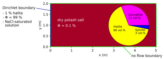
Figure 5.
Initial and boundary conditions: the inflow region is prescribed by a Dirichlet boundary (blue line); all other boundaries are impermeable (green lines); the models are initialized as dry with homogeneous potash salt (red, mineralogical composition shown) and halite inclusions according to Figure 6 (modified from Steding et al. [6]).

Table 1.
Potash salt mineral densities and dissolution properties (modified from Steding et al. [6]).
The 2D model height was 2 m, representing the typical thickness of potash seams in Germany, whereas the model width was 5 m with a discretization of 101 × 41 cells (Figure 5). At the start of the simulation, the entire model consisted of dry potash salt with a porosity of 0.1%. Natural caverns and leaching zones are commonly formed in the vicinity of tectonic fault systems which enable fluid migration [28]. Due to the fact that the ascending solution has to cross several rock salt layers before it reaches the potash seam, it is usually NaCl-saturated. To represent such a fault zone, a Dirichlet boundary was used (Figure 5). It maintains a constant solution composition and porosity at the left model boundary, assuming a high fluid and mineral exchange rate within the fault zone. The other boundaries were considered as impermeable without any pre-defined pressure gradient applied. The 2D model made use of the horizontally symmetric expansion of leaching zones to be expected if a potash seam has the same composition in both horizontal directions. Seen from the fault zone, the starting point of the leaching process, only one direction was simulated by taking advantage of the symmetry to reduce the required computational time.
If carnallite-bearing potash seams come into contact with NaCl-saturated brine, carnallite is always dissolved first, triggering the precipitation of sylvite and halite [29]. Equation (6) gives the overall reaction:
KMgCl3 × 6H2O + brine (NaCl) → KCl + NaCl (brine) + brine (MgCl2, KCl, NaCl)
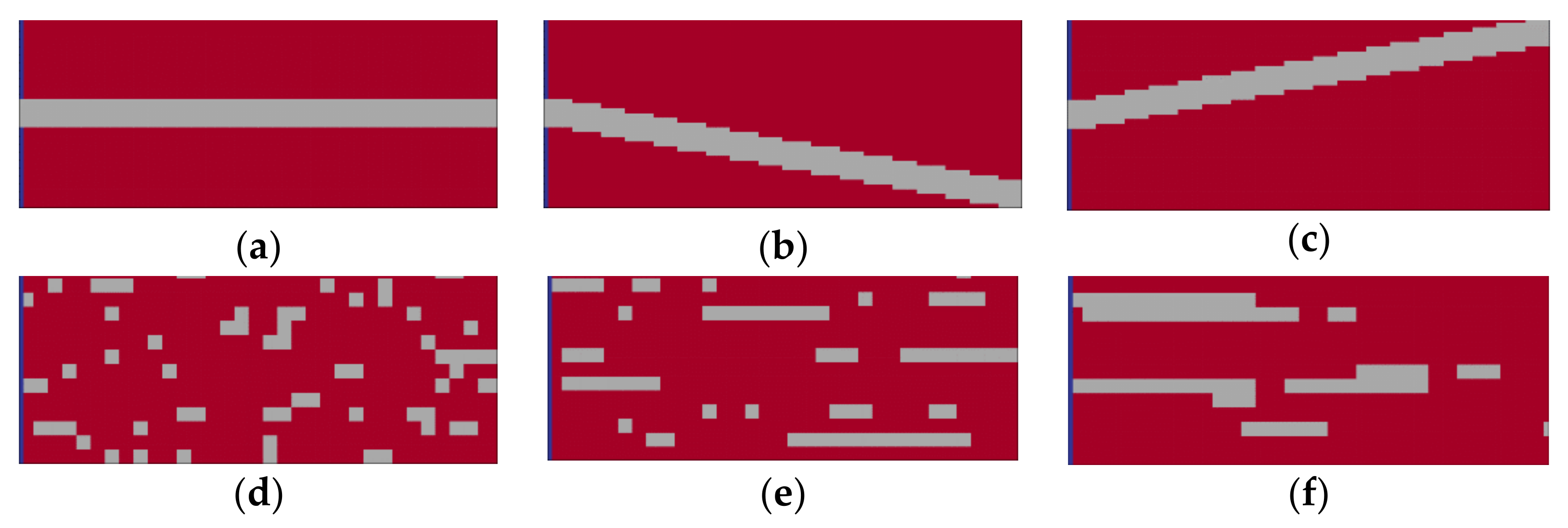
In contrast, halite is not dissolved from the potash seam [6,29], resulting in areas of pure halite (further referred to as halitic areas), acting as barriers to fluid flow. To investigate their influence on leaching zone evolution and hazard potentials, six generic rock distributions were considered. As shown in Figure 6, the first three represented a potash seam (red) with intersecting layers of halite (grey). These layers were 30 cm thick and showed inclinations of 0° or ±10°, respectively (Figure 6a–c). To ensure that boundary conditions are comparable, the layers always started at the same height at the center of the fault zone. In the other three cases, the potash seam contained halite inclusions ranging from 10 cm × 10 cm (Figure 6d) to nearly continuous, horizontal layers (Figure 6f). Their distribution was created with GSTools [30], using correlation lengths of 2:1, 17:0.5 and 34:1 in the horizontal direction. In all six cases, the halitic area made up between 13% and 15% of the potash seam and the surrounding potash salt was homogeneous with the composition shown in Figure 5. For comparison, an additional case without any halitic areas was considered.
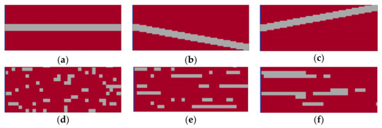
Figure 6.
Heterogeneous rock distributions examined: The homogeneous potash salt (red) shown in Figure 5 is veined by layers with (a) 0°, (b) +10°, (c) −10° inclination or inclusions of pure halite with correlation lengths of (d) 2:1, (e) 17:0.5 and (f) 34:1 that make up 13% to 15% of the potash seam.
For flow and transport calculations, the porosity–permeability relationship presented by Xie et al. [31] was applied. Carnallite is dissolved first and makes up >30% of the rock volume; therefore, a relatively large contact area between the solution and remaining minerals, sylvite and halite, can be assumed. Both minerals show the same maximum dissolution rate kmax as carnallite, facilitating a quick equilibration in the case of undersaturations. Therefore, non-equilibrated minerals were neglected in this study. Instead, sylvite and halite were immediately added to the equilibrated part Mineq as soon as the carnallite in their surroundings was dissolved. The diffusion coefficients of all four transported species Na+, Cl−, K+ and Mg2+ were assumed to be equal and constant: an average value of Df = 1.5 × 10⁻⁹ m2/s was chosen based on the study by Yuan-Hui and Gregory [32]. The fluid compressibility was set to cf = 4.6 × 10⁻¹⁰ 1/Pa. Temperature differences are negligible for a model height of 2 m; therefore, all simulations were undertaken at isothermal conditions at a temperature of 25 °C. Accordingly, the density-driven convective flow exclusively occurred due to dissolution and precipitation processes. The formation of leaching zones was simulated until the right model boundary was reached by the reaction front.
3. Results
3.1. Leaching Zone Growth
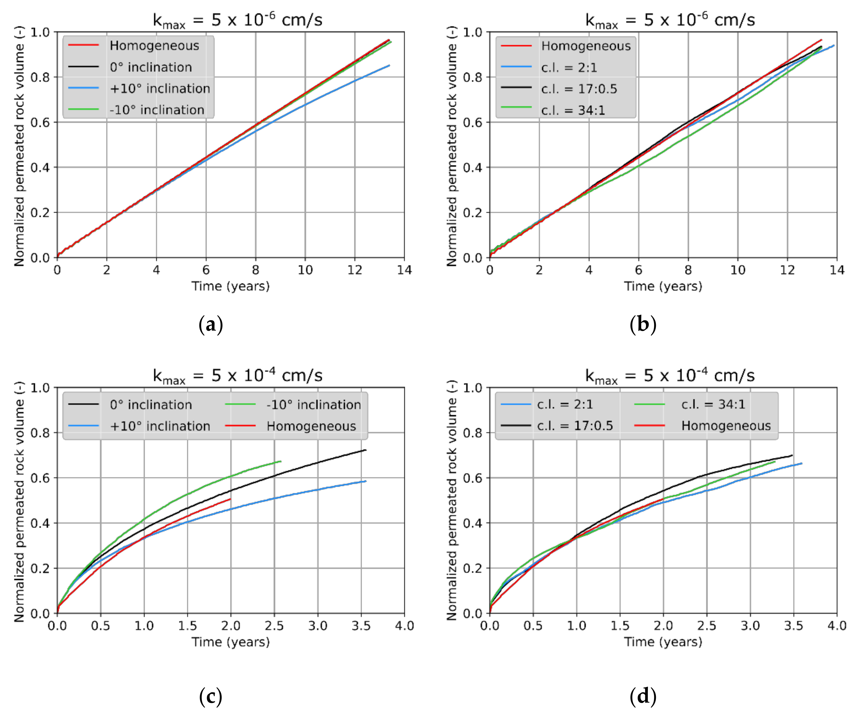
Figure 7 shows the evolution of the ratio between permeated and total rock volume (halitic areas not included). In cases of low dissolution rates (kmax = 5 × 10⁻⁶ cm/s), the leaching zone growth was nearly linear (Figure 7a,b). For all rock distributions, it took 13–14 years for the simulations to meet the stop criterion with 96% of the (non-halitic) rock being permeated. Only in the case of +10° inclination, the growth rate started to decrease after approximately six years (Figure 7a), with only 85% of the rock being permeated at the end. Halite inclusions led to a less regular growth rate compared to the homogeneous case, but large deviations from linear growth were not observed (Figure 7b).
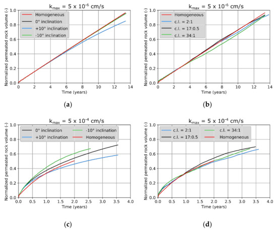
Figure 7.
Ratio between permeated and total (soluble) rock volume over time for (a,c) an intersecting halite layer and (b,d) halite inclusions (c.l., correlation length) compared to the homogeneous case.
In cases of high dissolution rates (kmax = 5 × 10⁻⁴ cm/s), the differences between rock distributions increase (Figure 7c,d). Along a homogeneous potash seam, the leaching zone expands to the right model boundary in two years, showing only a slight decrease in growth rate. However, only 50% of the rock become permeated, whereas the other half is not affected. In contrast, heterogeneous potash seams show permeation ratios of 59% to 72%, taking up to 3.6 years until the right model boundary is reached. Intersecting halite layers result in different evolutions depending on the inclination (Figure 7c). In cases of a 0° inclination, the permeation speed is slightly faster than for the homogeneous case, but the stop criterion is only met when 72% of the rock is permeated. Therefore, it takes 3.6 years instead of the 2 years in the homogenous case. In the case of a +10° inclination, the leaching zone growth is slower and only 60% of the rock is permeated within the same time period. An inclination of −10° (Figure 6c) causes the highest permeation speed, with 2.6 years required to reach a 67% permeation or the right model boundary. Potash seams with halite inclusions show a very similar permeation speed compared to homogeneous ones (Figure 7d). However, because 66% to 70% of the (soluble) rock is permeated (instead of 50%), it takes the reaction front almost twice as long to arrive at the right model boundary. Accordingly, heterogeneities slow down the leaching zone growth in horizontal direction by a factor of 1.25 to 1.8 in cases of high dissolution rates.
3.2. Péclet and Damköhler Numbers
In order to determine whether the systems are transport- or reaction-dominated, and if the transport is dominated by advection or diffusion, the dimensionless parameters of Péclet (Pe) and Damköhler (Da) can be used, allowing for a classification into four different cases which show different temporal and spatial evolutions of the leaching zone [6]. The Péclet number is determined from the flow velocity v, the diffusion coefficient Df and the characteristic length l, following Equation (7). Pe has to be calculated individually for each cell, because v varies in space (and time). l is approximated with the current width of the leaching zone, which varies over time in the vertical direction.
To determine if the system was dominated by advection (Pe > 2) or diffusion (Pe < 2), the median of all permeated cells was determined. All homogeneous and heterogeneous scenarios showed a median Péclet number which was clearly above two over the entire modeling period, i.e., all systems were advection-dominated. This means that diffusion was negligible as a transport process within the leaching zone, and the Damköhler number, which is defined as the ratio between reaction rate and transport velocity, could be calculated from the flow velocity v according to Equation (8). To calculate the reaction rate of each mineral, Equation (1) was used, considering the saturations of the inflowing solution. The studies of Field et al. [33] indicate that at the same flow velocity, low saturations cause transport-dominated systems (Da > 1), whereas high saturations result in reaction-dominated systems (Da < 1). The solution at the left boundary was NaCl-saturated; therefore, the reaction rate for halite was zero. In the cases of sylvite and carnallite, rate corresponds to kmax because the inflowing solution is highly undersaturated with respect to both minerals. The transport velocity corresponds to the flow velocity calculated by TRANSE.
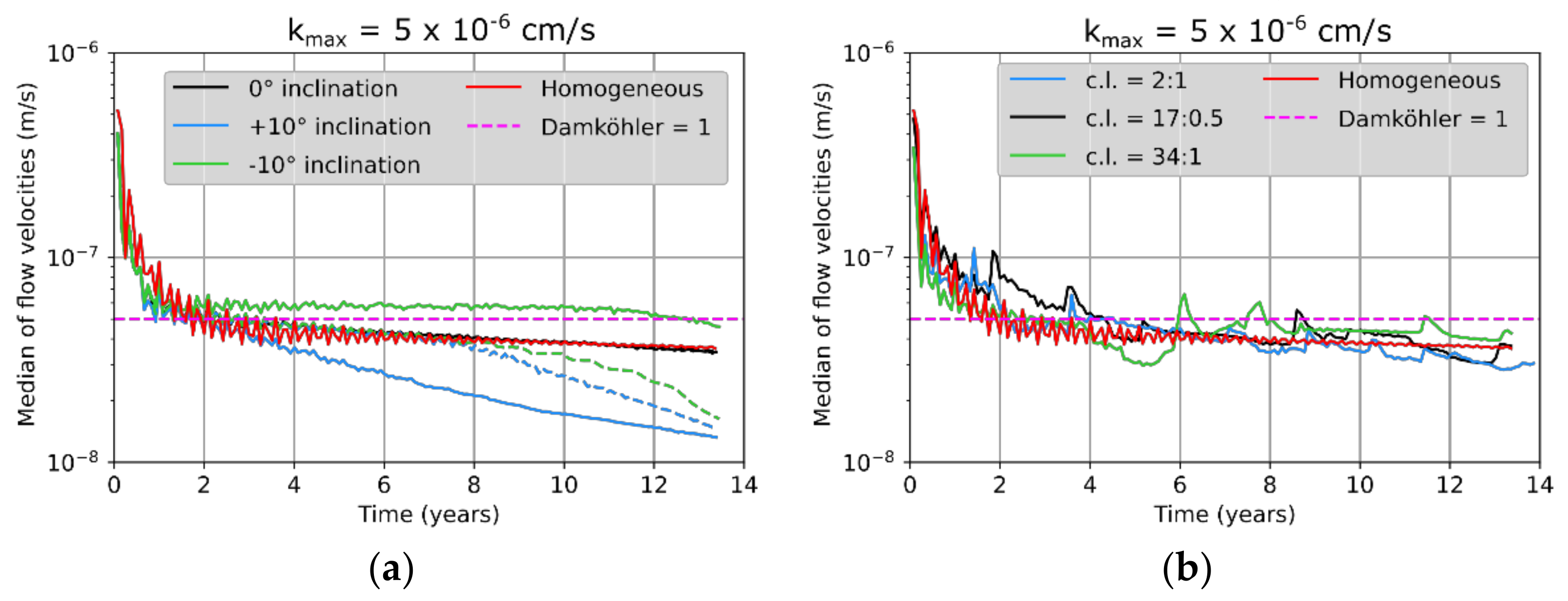
A Damköhler number for the system can be derived from kmax and the median of all flow velocities within the permeated area. The latter is divided into upper and lower halves in cases of intersecting halite layers. Figure 8 shows that the median always ranges between 10−6 m/s and 10−8 m/s. This means that for kmax = 5 × 10⁻⁴ cm/s, Da is always above one, whereas for kmax = 5 × 10⁻⁶ cm/s, Da falls below one if the flow velocity is above 5 × 10⁻⁸ m/s. In the case of homogeneous potash seams, this holds true during the first 2 years of simulation (Figure 8a,b). After that, the decrease in flow velocity results in a Damköhler number slightly above one, eventually equaling 1.4. If the potash seam is intersected by a horizontal halite layer, it takes 3 years to reach Da = 1 because the average flow velocity is slightly higher at the beginning (Figure 8a). Later, its decrease is stronger; thus, Da = 1.4 is eventually reached as well. Similar evolutions can be observed within the upper half of the potash seam if the intersecting halite layer is inclined. However, after 7–8 years, the flow velocity decrease becomes faster and Da becomes higher. On the other hand, flow velocities within the lower half are constantly lower for a +10° inclination and constantly higher for a −10° inclination. In the latter case, Da rises above one only after 13 years. In the case of halite inclusions, it partly takes more than 2 years to reach Da = 1, e.g., for the 17:0.5 distribution, and the evolution of the average flow velocity is less regular, resulting in several crossings of Da = 1 over time, e.g., for the 34:1 distribution (Figure 8b). However, the overall evolution of flow velocities is relatively similar to the homogeneous case.

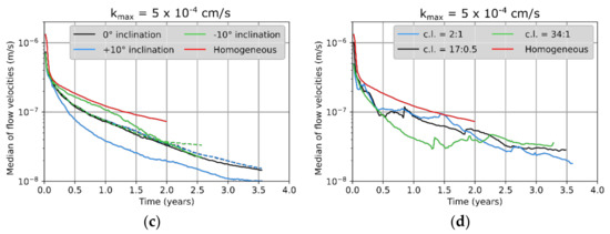
Figure 8.
Median of flow velocities over time for (a,c) an intersecting halite layer (solid line, below layer; dotted line, above layer) and (b,d) halite inclusions (c.l., correlation length) compared to the homogeneous case.
In contrast, kmax = 5 × 10⁻⁴ cm/s leads to larger deviations in flow velocity (Figure 8c,d). Thereby, heterogeneous potash seams generally show smaller flow velocities than homogeneous ones. In the case of a horizontal, intersecting layer, both halves show the same decrease in flow velocity over time, and after 2 years, the flow velocity amounts to approximately 50% of that in the homogeneous case (Figure 8c). The same evolution can be seen within the upper half of potash seams with intersecting layers at ±10° inclination. After 3.6 years, the flow velocities have decreased to 1.5 × 10⁻⁸ m/s, which represents only 20% of the final flow velocity in the homogeneous case. However, for a −10° inclination, the velocity decrease is reduced after 2 years, and the right model boundary is reached after only 2.6 years. Within the lower half of the potash seam, the average flow velocity is smaller compared to the upper half if the inclination of the intersecting layer is +10°. In contrast, it is generally higher in cases of −10° inclination. Thus, flow velocities within the lower half show an increased dependency on inclination. Heterogeneous potash seams with halite inclusions also show a clear trend towards flow velocity decreases over time (Figure 8d). However, phases of increase occur as well—especially for 34:1 distribution—which cannot be observed for homogeneous potash seams or intersecting layers.
3.3. Leaching Zone Evolution for Low Dissolution Rates (Da ≈ 1)
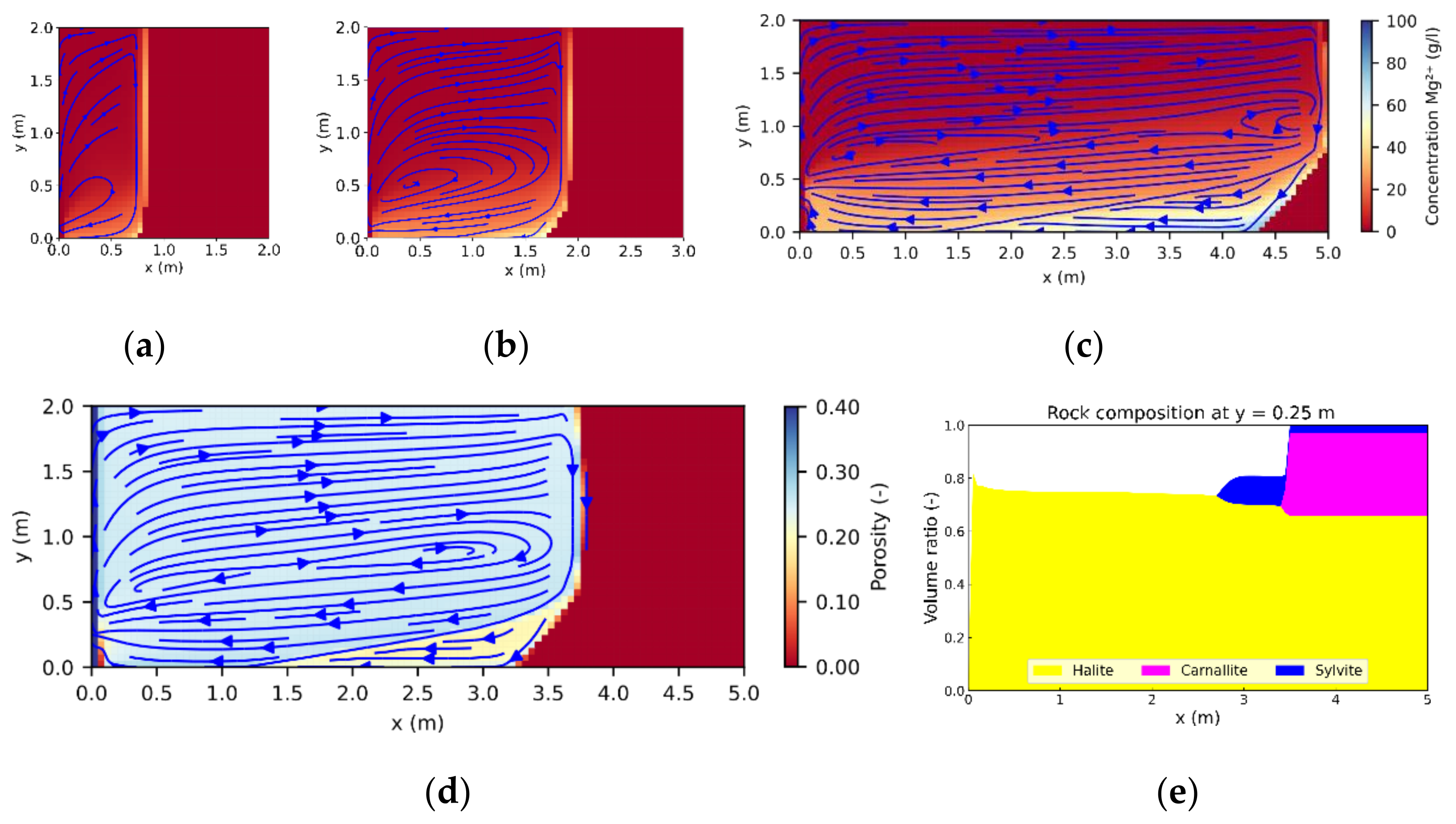
To evaluate the shift from reaction- (Da < 1) to transport-dominated (Da > 1) systems in the case of kmax = 5 × 10⁻⁶ cm/s, the distribution of Mg2+ after different time periods is shown in Figure 9. The Mg2+ concentration is a useful indicator for fluid density and saturation: an absence of Mg2+ usually represents a NaCl solution with a density of 1200 kg/m3, whereas a solution with >85 g/l Mg2+ (at 25 °C) has a density of >1270 kg/m3 and is fully saturated with respect to halite, sylvite and carnallite. In cases of homogeneous potash seams (Figure 9), the solution is highly undersaturated with regard to sylvite and carnallite along the entire dissolution front during the first two years. Accordingly, both minerals are fully dissolved and only halite remains. In contrast to halitic areas, the rock is fully permeated and porosity is high (≈30%) within these zones (further referred to as halite zones). The dissolution front is planar during that time, whereas concentration and density gradients are comparatively low. However, the Mg2+ concentration at the bottom increases, and after 2 years, when Da = 1 is reached, the dissolution of sylvite and carnallite is significantly reduced at the lower end of the dissolution front. As a result, a sylvinitic zone, consisting of halite and sylvite (Figure 9d,e), is formed next to it and an inclination of the dissolution front occurs. Over time, its upper end moves upwards (Figure 9b,c) and the sylvinitic zone with lower porosity grows. Additionally, a small barrier is formed next to the lower end of the inflow due to the precipitation of halite (Figure 9d).
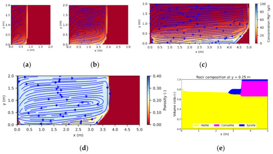
Figure 9.
Convection cell of a system shifted from a reaction- to a transport-dominated one: Mg2+ concentration distribution after simulation times of (a) 2 years, (b) 5 years and (c) 13.4 years; (d) porosity distribution and (e) mineralogical composition after 10 years for a homogeneous potash seam and kmax = 5 × 10⁻⁶ cm/s.
In cases of halite inclusions, the leaching zone evolution is basically similar to the homogeneous case. However, the more often the dissolution front is disturbed by inclusions, the more irregular it becomes (Figure 10a–c). The same applies to the sylvinitic zone within the lower area. Apart from that, sylvinitic zones now also occur above or behind inclusions and are often re-dissolved as soon as the flow regime changes and local Mg2+ concentrations decrease. A slower growth rate, which is usually associated with a sylvinitic zone next to the dissolution front, can now be observed within the upper area as well (Figure 10c). Generally, the convection cell is increasingly divided into smaller sub-cells, the broader the inclusions are. However, with regard to the shape and penetration depth of the leaching zone, differences compared to the homogeneous case are negligible.
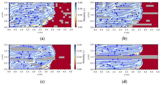

Figure 10.
Porosity distribution after a simulation time of 10 years for heterogeneous potash seams with halitic inclusions for the distributions (a) 2:1, (b) 17:0.5, (c) 34:1 and intersecting layers with (d) 0°, (e) +10°, (f) −10° inclination and kmax = 5 × 10⁻⁶ cm/s.
In the case of an intersecting, insoluble halite layer, the system is split up into two convection cells that evolve independently of each other. In the case of a horizontal layer (Figure 10d), both convection cells show nearly the same evolution compared to the homogeneous case (Figure 9). Although the sylvinitic zone is formed slightly later—after about 3 years instead of 2 years—it quickly covers a larger part of the dissolution front: after 10 years, approximately 50% of it, compared to 30% in the homogeneous case (Figure 9 and Figure 10d). However, the penetration depth at the upper end of the dissolution front is approximately the same. In contrast, the convection cells develop differently after some years if the intersecting layers are inclined (Figure 10e,f). Although the upper halves show similar flow velocities as in case of a horizontal layer during the first 7–8 years (Figure 8a), the sylvinitic zone is formed earlier and grows faster if the height increases (Figure 10e), whereas it does not occur at all if the height decreases (Figure 10f). The same applies to the formation of the barrier next to the inflow. On the other hand, an increasing height within the lower half results in the same sylvinitic zone and barrier formation, as in the case of a horizontal layer (Figure 10d,f), although flow velocities are higher and it takes 13 years to reach Da = 1 (Figure 8a). If the height within the lower half decreases, the sylvinitic zone starts forming after about 2.5 years, but grows relatively slow. After 10.5 years, it completely covers the dissolution front (Figure 10e), although it is only 1 m wide and 0.2 m high. From that point in time, the growth rate of the lower half is reduced, whereas flow velocities already show a significant decrease after 3 years (Figure 8a). In all other cases, the maximum penetration depth is the same within the upper and lower layer and the right model boundary is reached after 13.4 years.
3.4. Leaching Zone Evolution for High Dissolution Rates (Da > 1)
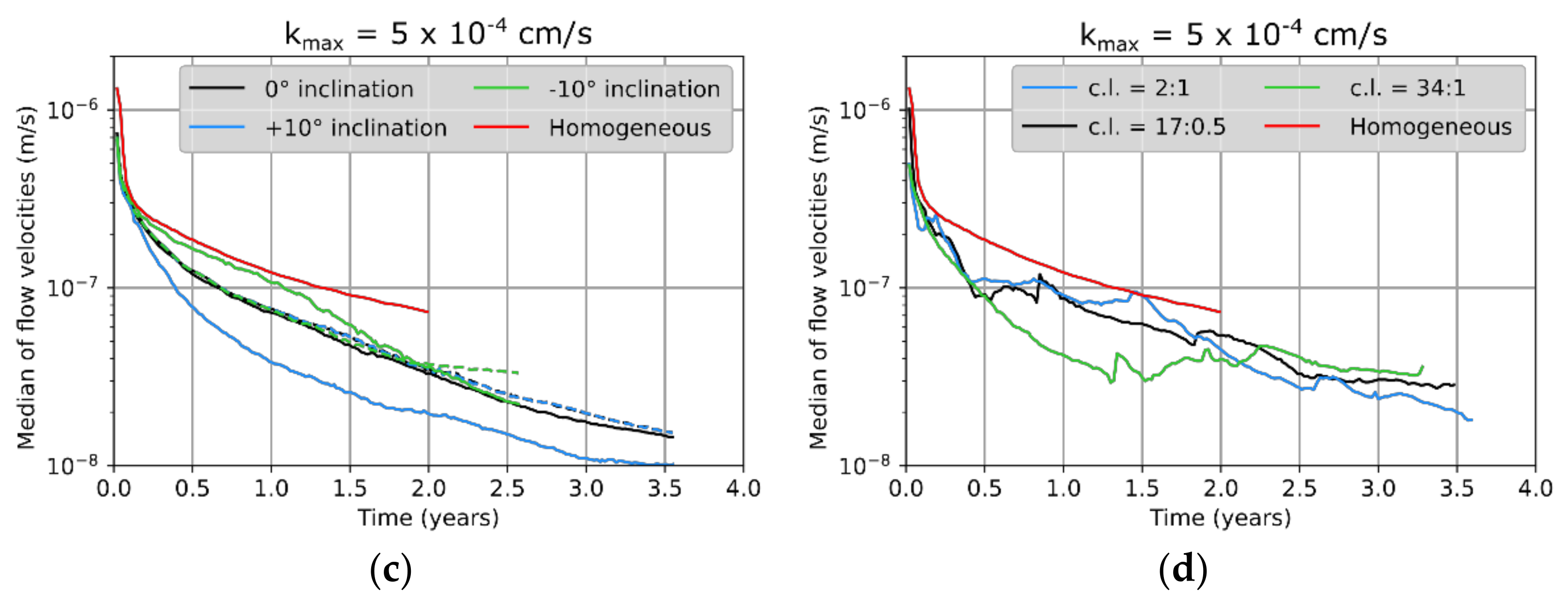
For kmax = 5 × 10⁻⁴ cm/s, the Damköhler number is clearly above one during the entire simulation time and a funnel-shaped leaching zone is formed, showing preferential dissolution within the upper half of the potash seam (Figure 11). Its width decreases nearly linearly from the top to the bottom. The lower part of the potash seam is not dissolved, resulting in an increased flattening of the dissolution front over time. As indicated in Figure 7c,d, the expansion becomes slower over time: although the leaching zone penetrates 3 m deep into the seam in the first year, it proceeds only two more meters within the second year. The precipitation of halite next to the left model boundary leads to the formation of a flow barrier within the lower half of the potash seam. Close to the entire dissolution front, a sylvinitic zone is formed (Figure 11a, yellow). Its maximum width in the horizontal direction is reached at the height of the barrier top. Basically, two different solution compositions exist within the leaching zone. The first one contains almost no Mg2+ and can be found within the halite zone (Figure 11a, blue), whereas the second one shows Mg2+ concentrations of >70 g/l and is present within the sylvinitic zone (Figure 11a, yellow). The border reaches from the upper end of the dissolution front to the top of the barrier and represents an area with large concentration gradients. Thus, there is a large density gradient at the border as well, representing the driving force of the free convection. Figure 11a shows that above this border, fluid flow proceeds mainly from left to right, whereas below it, the (highly saturated) solution is moving from the dissolution front back towards the left boundary.
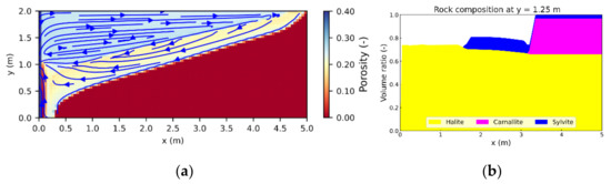
Figure 11.
Convection cell of a fully transport-dominated system: (a) porosity distribution and (b) mineralogical composition after a simulation time of 2 years for a homogeneous potash seam and kmax = 5 × 10⁻⁴ cm/s.
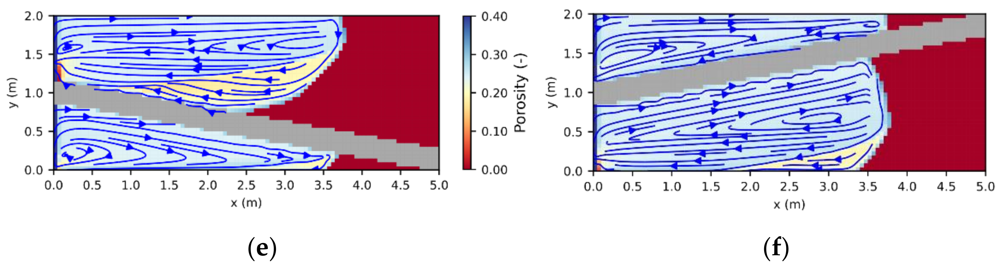
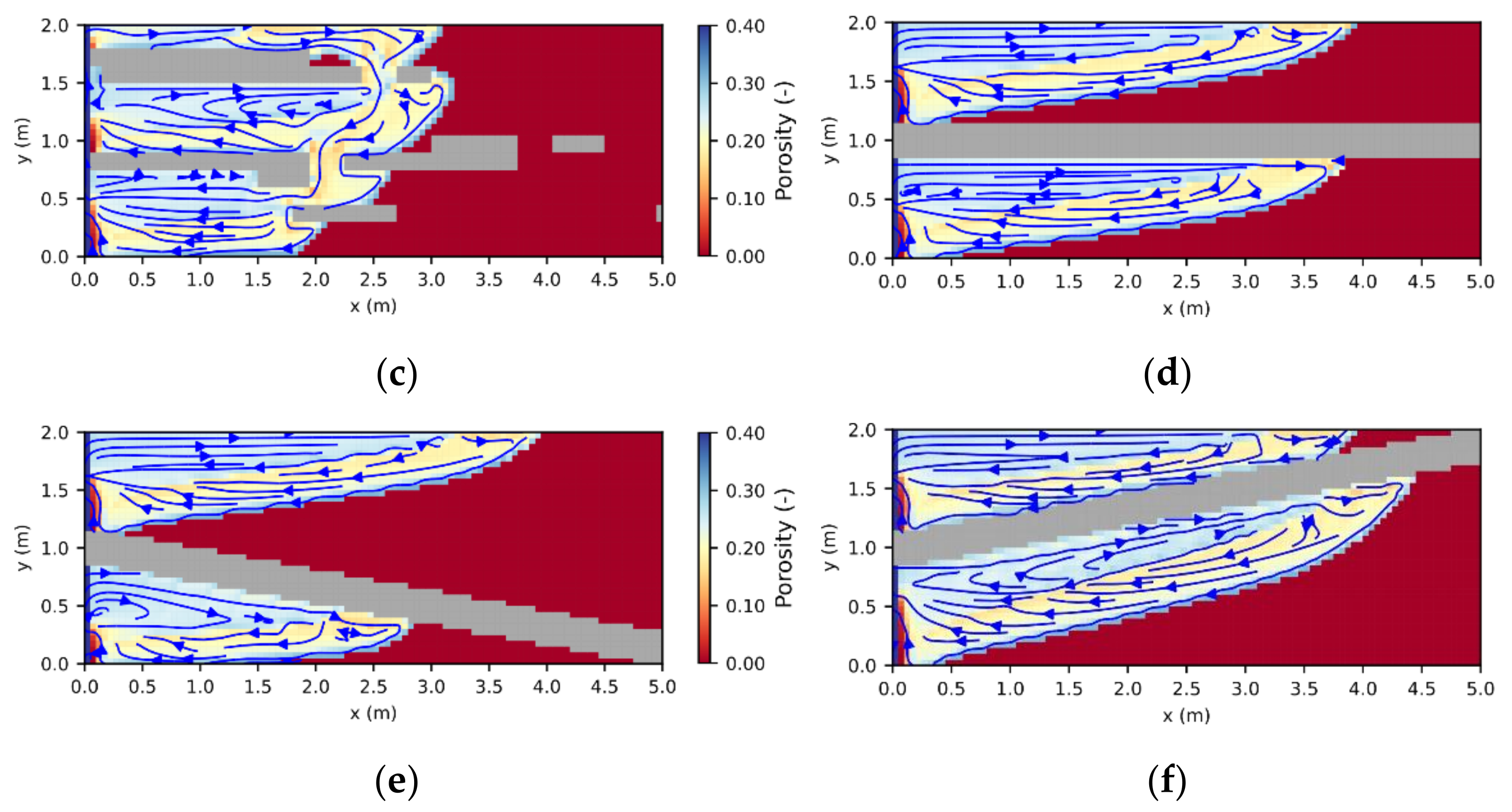
In cases of small and medium-sized halite inclusions, the flow field becomes less regular but still shows one main convection cell with undersaturated inflowing solution, mainly present within the upper-left area of the leaching zone, and highly saturated outflowing solution along the dissolution front and within the lower area (Figure 12a,b). Accordingly, the shape of the sylvinitic zone and barrier remains basically similar to the homogeneous case. However, zones containing only halite now also occur within the lower half of the leaching zone behind the barrier. In return, wide sylvinitic zones can occur in the upper half, especially above inclusions (Figure 12b). Neither the inclination of the dissolution front nor of the border between the halite and sylvinitic zone is linear anymore, and the lower end of the dissolution front is about 1 m away from the inflow compared to 0.25 m in the homogeneous case (Figure 11a and Figure 12a,b). For broader inclusions, the flow field shows three smaller convection cells after 10 years, with each having its own barrier at the left (Figure 12c). The same applies to the sylvinitic zone. The dissolution front is subdivided into 3–4 sections with different penetration depths. Thereby, the upper one shows lower dissolution rates than the one below, leading to a recess at 1.6 m height. However, this phenomenon quickly disappears as soon as the upper half of the dissolution front is not subdivided anymore, and the flow regime changes accordingly. Between large inclusions, the flow is not disturbed and the dissolution front as well as the borders between halite and sylvinitic zones are nearly as regular as in the homogeneous case (Figure 11a). However, the overall inclination of the dissolution front is much steeper. As a result, the same permeation speed leads to smaller penetration depths within the upper part of the potash seam after 2 years, but higher permeation ratios at the end for all cases of halite inclusions (Figure 7d). Here, the right model boundary is reached after 3.3 years (34:1) to 3.6 years (2:1).
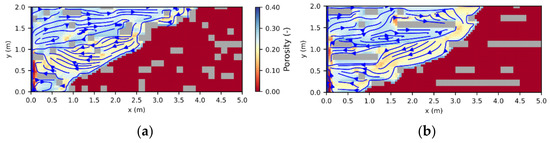

Figure 12.
Porosity distribution after a simulation time of 2 years for heterogeneous potash seams with halitic inclusions for distributions of (a) 2:1, (b) 17:0.5, (c) 34:1 and intersecting layers with (d) 0°, (e) +10°, (f) −10° inclination and kmax = 5 × 10⁻⁴ cm/s.
The leaching zones above intersecting layers show nearly similar evolutions in penetration depth regardless of the inclination (Figure 12d–f). If the height is constant or increases, shape and flow velocities evolve similarly (Figure 12d,e and Figure 8d), whereas in cases of decreasing height, the dissolution front follows the intersecting layer (Figure 12f) and the penetration speed slightly decreases as the height falls below 0.25 m. Compared to the homogeneous case, the width of the leaching zone shows a lower decrease within the upper half and a greater decrease within the lower half, resulting in higher permeation ratios (Figure 7c). Only if the height increases is a large area of undissolved potash salt maintained between the intersecting layer and the upper leaching zone, leading to an overall permeation ratio of 59% (compared to >70% for 0° and −10° inclination) at the end of the simulation time (Figure 7c and Figure 12e). After 2 years, the barrier covers about half of the upper in- and outflow region and the right model boundary is reached after 3.5 years. However, in the case of a −10° inclination, the lower leaching zone grows faster than the upper one (Figure 12f). Thus, the right model boundary is already reached after 2.6 years. In contrast, the +10° inclination results in smaller growth rates within the lower half (Figure 12e). Generally, layers with increasing height grow faster, whereas layers with decreasing height show higher permeation ratios (Figure 12e,f). Compared to the homogeneous case, sylvinitic zones (yellow) are slightly broader at the upper end of the dissolution front in all cases of intersecting layers.
4. Discussion
The results show that the influence of insoluble inclusions and intersecting layers strongly depends on the dissolution rate of the soluble minerals. In cases of low dissolution rates (kmax = 5 × 10⁻⁶ cm/s), the evolution of the leaching zone is only slightly affected (Figure 7a,b and Figure 10), although local and average flow velocities are significantly changed (Figure 8a,b). In contrast, heterogeneities lead to a reduction in penetration depth (Figure 12) and higher permeation ratios (Figure 7c,d) if dissolution rates are high (kmax = 5 × 10⁻⁴ cm/s). These differences can be explained by a distinction between reaction-dominated and transport-dominated systems. A fully reaction-dominated system (Da << 1) is given if the effective dissolution rates of sylvite and carnallite according to Equation (1) correspond to the maximum dissolution rate, i.e., if their saturation only shows a very slight increase along the dissolution front. In this case, the dissolution front is planar and neither local nor overall changes in flow velocity affect the growth rate of the leaching zone: it is entirely controlled by the reaction speed. This case is given for kmax = 5 × 10⁻⁶ cm/s at the start of the simulation. However, after some years, the saturations along the dissolution front become high enough to significantly reduce the dissolution rate of sylvite and carnallite, making the system only partly reaction-dominated (Da ≈ 1). The reason for that can be a decrease in flow velocity or an increase in the length of the dissolution front. As a result, the dissolution front becomes inclined and a sylvinitic zone as well as a barrier are formed (Figure 9). If the entire dissolution front is inclined and covered by a sylvinitic zone, the system is fully transport-dominated (Da >> 1), as given for kmax = 5 × 10⁻⁴ cm/s. These systems are much more sensitive to changes in flow velocity. Therefore, they are much more affected by heterogeneities influencing both the local distribution and the average flow velocity (Figure 8, Figure 10 and Figure 12).
The Damköhler number is a useful indicator to determine if a system is dominated by reaction or transport [6,34,35]. Generally, the simulation results show that an overall Da calculated from the average flow velocity and the saturation-dependent dissolution rate of the inflowing solution corresponds to the observed leaching zone shapes. In cases of kmax = 5×10⁻⁴ cm/s, Da >> 1 is given and a funnel shape can be observed, including a barrier at the left and a sylvinitic zone along the entire dissolution front (Figure 11). These are typical indicators for a transport-dominated system [6]. In cases of kmax = 5 × 10⁻⁶ cm/s, the dissolution front is planar in the beginning when Da < 1, whereas it becomes inclined as Da rises above one, with a sylvinitic zone and barrier rising from the bottom (Figure 8a,b and Figure 9a–c). However, insoluble inclusions make it more difficult to identify this point in time, because the average flow velocity evolves less regularly (Figure 8b) and strong local deviations occur, resulting in small sylvinitic zones near the inclusions and a more irregular dissolution front (Figure 10a–c). In cases of intersecting layers, Da has to be determined for each sub-system or convection cell, and if the layer is inclined, the time period in which Da rises above one does no longer correlate with the formation of sylvinitic zones and barriers (Figure 8a and Figure 10d–f). From our point of view, the reason for this is a change in the length of the dissolution front: if it increases, higher saturations can be reached at the bottom without a change in flow velocity, and vice versa. All in all, the larger the heterogeneities are in size, the less appropriate an overall Damköhler number is to determine if the system is dominated by reactions or transport. Additionally, it has to be noted that complex systems containing several minerals can be reaction- and transport-dominated at the same time: if the maximum dissolution rate kmax or the saturations of the inflowing solution vary a lot for different minerals, some of them will show Da > 1, whereas others show Da < 1. Accordingly, the Damköhler number has to be calculated individually for each mineral and an internal contact area between equilibrated and non-equilibrated minerals has to be defined (Figure 4) to reproduce the formation of several dissolution fronts, as observed by Ahoulou et al. [26]. In this case, heterogeneities are expected to mainly influence the dissolution pattern of minerals with Da > 1.
Heterogeneities also affect the hazard potential of leaching zones by influencing the growth rate, shape and permeation ratio. In this context, higher growth rates are associated with faster expansion of the leaching zone and an increasing risk of mine flooding or integrity loss of a cavern. Higher permeation ratios or porosities also increase the hazard potential because they result in a lower mechanical stability as well as larger solution amounts stored per meter leaching zone. The results show that for Da >> 1, insoluble inclusions mainly affect the shape: at the top, the dissolution front is progressing relatively slowly, whereas at the bottom, dissolution rates are higher compared to the homogeneous case (Figure 11 and Figure 12a–c). As a result, the permeation speed is basically the same (Figure 7d), but the dissolution front is steeper, and it takes 1.65–1.8 times longer until the right model boundary is reached. It is important to note that the distribution of insoluble inclusions does not have a significant influence if their volume ratio is identical. Although broader inclusions increasingly split up the convection cell into smaller ones and lead to a more irregular average flow velocity, the overall evolution is always quite similar (Figure 7d, Figure 8d and Figure 12a–c). Thereby, the leaching zone growth in the horizontal direction is slower compared to the homogeneous case, but the permeation ratio is higher at the end of the simulation, which can become more critical with regard to mechanical stability. In the case of one continuous insoluble layer, the leaching zone consists of two independent convection cells, showing the same regular dissolution front, sylvinitic zone and barrier as in the homogeneous case. However, flow velocities and permeation speed are more similar to those of insoluble inclusions (Figure 7c, Figure 8c and Figure 12d). Inclined, intersecting layers particularly influence the flow velocity within the lower half (Figure 8c). Thereby, negative inclinations increase the flow velocity, resulting in faster leaching zone growth compared to the upper half (Figure 12f), and vice versa. The evolution of the upper half is basically not influenced (Figure 12e,f). However, the amount of undissolved potash rock is larger with increasing height, resulting in relatively small permeation ratios (Figure 7c). In summary, an intersecting layer with negative inclination is the most critical distribution of insoluble inclusions, leading to higher permeation ratios and only slightly smaller growth rates in the horizontal direction compared to the homogeneous case.
Field observations indicate that the formation of caverns and leaching zones in salt rock is usually dominated by transport. According to Koch and Vogel [29], the upper half of a potash seam is often preferentially dissolved, and natural leaching zones within carnallitic rock are mostly divided into a halite zone near the inflow region and a sylvinitic zone close to the dissolution front. These observations agree with the results for a transport-dominated system (kmax = 5 × 10⁻⁴ cm/s) of homogeneous rock composition (Figure 11). In the case of intersecting layers from pure halite, Koch and Vogel [29] assumed a split into several dissolution fronts with different penetration depths. A similar phenomenon has been observed in solution mining: if several insoluble layers cross the salt body, the resulting cavern shape resembles an inverted Christmas tree [7]. The same shape is described by Fokker [10] for technical caverns crossing different (potash) salt layers. Furthermore, Fokker [10] implies that inclined layers cause an asymmetric shape, whereby the growth rate is faster in the direction of upward-directed inclination. These descriptions all correspond to the simulation results for a transport-dominated system with intersecting halite layers (Figure 12d–f). However, time frames for the evolution of natural leaching zones are not available. Regarding insoluble inclusions, laboratory experiments conducted by Gechter et al. [36] and Field et al. [33] confirm that the cavern shape becomes increasingly distorted, and notches occur at the dissolution front if insoluble lenses impede regular fluid flow (Figure 12a–c). Additionally, findings that inclusions do not reduce the amount of dissolved/permeated rock per time, but only its distribution (Figure 7d), are consistent [36]. Reaction-dominated systems with (nearly) planar dissolution fronts only occur if the inflowing solution is already highly saturated with respect to the present salt minerals [33]. In this case, significantly slower growth rates as well as an increased influence of rock fabric were observed. The first finding agrees with our simulation results (Figure 7), whereas the second one could not be reproduced (Figure 10a–c). Overall, there is a good correlation between literature data and model results regarding the influence of heterogeneities. However, temporal scaling is still uncertain, and more data are required for comprehensive quantitative model validation.
Finally, the results reveal how saturation-dependent dissolution rates affect barrier formation and leaching zone shape. In the case of fully reaction-dominated systems (Da << 1), there is no difference compared to constant dissolution rates because kmax is always reached. In contrast, transport-dominated systems show a more linear decrease in width from the top to the bottom, because the effective dissolution rate decreases along the dissolution front. Therefore, a longer distance is required until the solution is fully saturated and the transition from dissolved to undissolved sections of the potash seam is less sharp compared to constant dissolution rates [6]. Additionally, the barrier next to the inflow is smaller, resulting in a less decreasing flow velocity and growth rate over time. Thus, saturation-dependent dissolution rates lead to a wider extension, and therefore a higher hazard potential of the leaching zone in the long term. Furthermore, they intensify the coupling between chemical reactions and transport. Next to the dissolution front, where strong concentration gradients occur, changes in advection, diffusion or dispersion immediately affect the saturations, and therefore the effective dissolution rates. In return, the dissolved mineral amounts affect transport parameters such as brine density, viscosity and diffusion coefficients. An even stronger coupling would be achieved if kmax is treated as a function of flow velocities. Several studies indicate that for fast-dissolving minerals, such as most potash salts, the dissolution rate is controlled by the transport across a so-called diffusive boundary layer which is formed at the mineral–fluid interface [19,23,27]. Thereby, higher fluid flow velocities induce a decrease in thickness of the boundary layer, and therefore higher dissolution rates of the minerals. As a result, kmax varies locally and heterogeneities may have a stronger effect. However, the approach uses input parameters, such as the reaction rate constant, which are currently not known for many potash minerals. Furthermore, knowledge about the flow field at pore scale and the bulk concentrations outside the boundary layer are required [37]. Both are hard to determine by continuum-scale models which cannot exactly reproduce the concentration distribution at the dissolution front. By using average saturations to calculate the dissolution rates, artificial mixing is always generated, influencing the leaching zone shape or the fluid flow path until full saturation is reached. Accordingly, a calibration of the model based on experimental data is crucial. Overall, the simulation results show that the saturation dependency of dissolution rates has a significant influence on the leaching zone evolution in cases of partly or fully transport-dominated systems (Da ≥ 1), and therefore needs to be considered when investigating further scenarios.
5. Conclusions
The scenario analysis for a generic potash seam has significantly improved the understanding of the influence of insoluble inclusions and intersecting layers on the evolution of leaching zones. It was shown that in the case of advection- and reaction-dominated systems (Pe > 2 and Da < 1), growth rate, shape and porosity of the leaching zone are basically identical in heterogeneous and homogeneous cases, meaning that heterogeneities can be neglected with regard to risk assessment. In advection- and transport-dominated systems (Pe > 2 and Da > 1), the amount of potash salt permeated over time is similar in both cases, but the shape of the leaching zones is different. As a result, the upper end of the dissolution front (s) moves forward 1.8 times slower in the heterogeneous case, regardless of the distribution of insoluble areas. Consequently, heterogeneities decrease the hazard potential. To account for this effect, only the volume ratio of insoluble minerals has to be known, representing a major advantage in practice because exact distributions are seldom known. Only in the case of intersecting layers with negative inclination, a smaller reduction in growth rate and an asymmetric expansion of the leaching zone need to be considered. Neglecting heterogeneities usually generates a safety margin in the overall assessment, unless the increase in permeation ratio endangers the mechanical stability of the leaching zone. If insoluble layers and/or large inclusions collapse, new fluid flow paths may be formed, significantly increasing leaching zone growth rates as well as hazard potentials.
Literature data indicate that most natural systems are transport-dominated. However, the Damköhler number needs to be calculated individually for each mineral and, in the case of intersecting layers, also for each separate leaching zone to reliably assess the influence of heterogeneities and to predict further leaching zone evolution. Heterogeneities, especially inclined intersecting layers, influence local and average fluid flow velocities; therefore, the validity of a global Damköhler number is reduced. Instead, the occurrence of funnel shapes, barriers and sylvinitic zones (in the case of carnallitic potash salt) should be used to determine if a system is dominated by reaction (Da < 1) or transport (Da > 1).
The extension of the reactive transport model by variable saturation-dependent dissolution rates has improved its accuracy with regard to the leaching zone shape, growth rate and barrier formation. It is shown that constant dissolution rates overestimate barrier formation, and therefore underestimate hazard potentials in the long-term. In the next step, it is planned to not only distinguish between insoluble and highly soluble minerals, but to also include more slowly dissolving minerals such as anhydrite (CaSO4) or kieserite (MgSO4·H2O) into the assessment by using individual maximum dissolution rates. In doing so, the effects of mineral heterogeneity can be investigated in further detail. However, for many secondary minerals occurring in these complex quinary or hexary systems, kmax is unknown. Furthermore, a dependency on the local flow velocity is expected to intensify the coupling between chemical reactions and transport. Therefore, laboratory and field measurement data are required to calibrate kmax. With these extensions, the reactive transport model can be principally applied to any study area for prediction of the preferential expansion of leaching zones along potash seams and assessment of their hazard potentials.
Author Contributions
Conceptualization, M.K. and S.S.; methodology, S.S. and T.K.; software, S.S. and T.K.; validation, S.S.; formal analysis, S.S.; investigation, S.S.; resources, M.K.; writing—original draft preparation, S.S.; writing—review and editing, S.S., T.K. and M.K.; visualization, S.S.; supervision, T.K. and M.K. All authors have read and agreed to the published version of the manuscript.
Funding
This research was a contribution to the GEO:N project ProSalz and supported by the Federal Ministry of Education and Research, Germany, grant number 03A0014A.
Institutional Review Board Statement
Not applicable.
Informed Consent Statement
Not applicable.
Acknowledgments
The authors would like to thank the German Federal Ministry of Education and Research for the financial support of the project. Furthermore, we thank Axel Zirkler and T. Radtke from K + S for many informative discussions and useful advice regarding the model conceptualization.
Conflicts of Interest
The authors declare no conflict of interest. The funders had no role in the design of the study; in the collection, analyses, or interpretation of data; in the writing of the manuscript, or in the decision to publish the results.
References
- Warren, J.K. Salt usually seals, but sometimes leaks: Implications for mine and cavern stabilities in the short and long term. Earth Rev. 2017, 165, 302–341. [Google Scholar] [CrossRef]
- Prugger, F.F.; Prugger, A.F. Water problems in Saskatchewan potash mining—What can be learned from them? Undergr. Min. 1991, 84, 58–66. [Google Scholar]
- Boys, C. A Geological Approach to Potash Mining Problems in Saskatchewan, Canada. Explor. Min. Geol. 1993, 2, 129–138. [Google Scholar]
- Keime, M.; Charnavel, Y.; Lampe, G.; Theylich, H. Obstruction in a salt cavern: Solution is dissolution. In Proceedings of the 25th World Gas Conference, Kuala Lumpur, Malaysia, 4–8 June 2012. [Google Scholar]
- Mengel, K.; Röhlig, K.J.; Geckeis, H. Endlagerung radioaktiver Abfälle. Chemie Unserer Zeit 2012, 46, 208–217. [Google Scholar] [CrossRef]
- Steding, S.; Kempka, T.; Zirkler, A.; Kühn, M. Spatial and temporal evolution of leaching zones within potash seams reproduced by reactive transport simulations. Water 2021, 13, 168. [Google Scholar] [CrossRef]
- Thoms, R.L.; Gehle, R.M. Non-halites and fluids in salt formations, and effects on cavern storage operations. Geotech. Spec. Publ. 1999, 90, 780–796. [Google Scholar]
- Li, J.; Shi, X.; Yang, C.; Li, Y.; Wang, T.; Ma, H. Mathematical model of salt cavern leaching for gas storage in high-insoluble salt formations. Sci. Rep. Nat. 2018, 8, 372. [Google Scholar] [CrossRef] [PubMed]
- Jinlong, L.; Wenjie, X.; Jiangjing, Z.; Wei, L.; Xilin, S.; Chunhe, Y. Modeling the mining of energy storage salt caverns using a structural dynamic mesh. Energy 2020, 193, 116730. [Google Scholar] [CrossRef]
- Fokker, P.A. The behaviour of salt and salt caverns. Doctoral Dissertation, TU Delft, Delft, The Netherlands, 24 January 1995. Available online: http://resolver.tudelft.nl/uuid:6847f8e4-3b09-4787-be02-bcce9f0eed06 (accessed on 25 June 2021).
- Liu, M.; Shabaninejad, M.; Mostaghimi, P. Impact of mineralogical heterogeneity on reactive transport modelling. Comput. Geosci. 2017, 104, 12–19. [Google Scholar] [CrossRef]
- Wei, W.; Varavei, A.; Sanaei, A.; Sepehrnoori, K. Geochemical Modeling of Wormhole Propagation in Carbonate Acidizing Considering Mineralogy Heterogeneity. SPE J. 2019, 24, 2163–2181. [Google Scholar] [CrossRef]
- Kempka, T. Verification of a Python-based TRANsport Simulation Environment for density-driven fluid flow and coupled transport of heat and chemical species. Adv. Geosci. 2020, 54, 67–77. [Google Scholar] [CrossRef]
- Parkhurst, D.L.; Appelo, C.A.J. Description of Input and Examples for PHREEQC Version 3—A Computer Program for Speciation, Batch-reaction, One-dimensional Transport, and Inverse Geochemical Calculations. In Techniques and Methods; U.S. Geological Survey: Reston, VA, USA, 2013. [Google Scholar]
- Altmaier, M.; Brendler, V.; Bube, C.; Marquardt, C.; Moog, H.C.; Richter, A.; Scharge, T.; Voigt, W.; Wilhelm, S.; Wilms, T.; et al. THEREDA, Thermodynamische Referenz-Datenbasis; Report 265; Gesellschaft für Anlagen–Und Reaktorsicherheit (GRS): Braunschweig, Germany, 2011; 63p. [Google Scholar]
- Durie, R.; Jessen, F. Mechanism of the Dissolution of Salt in the Formation of Underground Salt Cavities. Soc. Pet. Eng. J. 1964, 4, 183–190. [Google Scholar] [CrossRef]
- Röhr, H.U. Lösungsgeschwindigkeiten von Salzmineralen beim Ausspülen von Hohlräumen im Salz. Kali Steinsalz 1981, 8, 103–111. [Google Scholar]
- Palandri, J.L.; Kharaka, Y.K. A Compilation of Rate Parameters of Water—Mineral Interaction Kinetics for Application to Geochemical Modeling; U.S. Geological Survey (USGS): Menlo Park, CA, USA, 2004; Available online: http://www.dtic.mil/cgi-bin/GetTRDoc?Location=U2&doc=GetTRDoc.pdf&AD=ADA440035 (accessed on 5 April 2021)Report 2004/1068.
- Alkattan, M.; Oelkers, E.; Dandurand, J.; Schott, J. Experimental studies of halite dissolution kinetics, 1 The effect of saturation state and the presence of trace metals. Chem. Geol. 1997, 137, 201–219. [Google Scholar] [CrossRef]
- Steding, S.; Zirkler, A.; Kühn, M. Geochemical reaction models quantify the composition of transition zones between brine occurrence and unaffected salt rock. Chem. Geol. 2020, 532, 119349. [Google Scholar] [CrossRef]
- Yang, X.; Liu, X.; Zang, W.; Lin, Z.; Wang, Q. A Study of Analytical Solution for the Special Dissolution Rate Model of Rock Salt. Adv. Mater. Sci. Eng. 2017, 1–8. [Google Scholar] [CrossRef] [Green Version]
- Hoppe, H.; Winkler, F. Beitrag zur Lösekinetik von Mineralien der Kaliindustrie. Wiss. Z. Tech. Hochsch. Chem. Leuna-Mersebg. 1974, 16, 23–28. [Google Scholar]
- De Baere, B.; Molins, S.; Mayer, K.U.; François, R. Determination of mineral dissolution regimes using flow-through time-resolved analysis (FT-TRA) and numerical simulation. Chem. Geol. 2016, 430, 1–12. [Google Scholar] [CrossRef] [Green Version]
- Dreybrodt, W.; Buhmann, D. A mass transfer model for dissolution and precipitation of calcite from solutions in turbulent motion. Chem. Geol. 1991, 90, 107–122. [Google Scholar] [CrossRef]
- Raines, M.A.; Dewers, T.A. Mixed transport/reaction control of gypsum dissolution kinetics in aqueous solutions and initiation of gypsum karst. Chem. Geol. 1997, 140, 29–48. [Google Scholar] [CrossRef]
- Ahoulou, A.W.A.; Tinet, A.J.; Oltéan, C.; Golfier, F. Experimental Insights into the Interplay Between Buoyancy, Convection, and Dissolution Reaction. J. Geophys. Res. Solid Earth 2020, 125, 1–18. [Google Scholar] [CrossRef]
- Dutka, F.; Starchenko, V.; Osselin, F.; Magni, S.; Szymczak, P.; Ladd, A.J.C. Time-dependent shapes of a dissolving mineral grain: Comparisons of simulations with microfluidic experiments. Chem. Geol. 2020, 540, 119459. [Google Scholar] [CrossRef]
- Höntzsch, S.; Zeibig, S. Geogenic caverns in rock salt formations—A key to the understanding of genetic processes and the awareness of hazard potential. In Earth System Dynamics, GeoFrankfurt 2014, Frankfurt a.M., Germany, Sept 2014; Schweizerbart Science Publishers: Stuttgart, Germany, 2014. [Google Scholar]
- Koch, K.; Vogel, J. Zu den Beziehungen von Tektonik, Sylvinitbildung und Basaltintrusionen im Werra-Kaligebiet. In Freiberger Forschungshefte; VEB Deutscher Verlag für Grundstoffindustrie: Leipzig, Germany, 1980; C 347; 104p. [Google Scholar]
- Müller, S.; Schüler, L. GeoStat-Framework/GSTools. Zenodo 2019. [Google Scholar] [CrossRef]
- Xie, M.; Kolditz, O.; Moog, H. A geochemical transport model for thermo-hydro-chemical (THC) coupled processes with saline water. Water Resour. Res. 2011, 47, W02545. [Google Scholar] [CrossRef]
- Yuan-Hui, L.; Gregory, S. Diffusion of ions in sea water and in deep-sea sediments. Geochim. Cosmochim. Acta 1974, 38, 703–714. [Google Scholar] [CrossRef]
- Field, L.; Milodowski, A.E.; Evans, D.; Palumbo-Roe, B.; Hall, M.R.; Marriott, A.L.; Barlow, T.; Devez, A. Determining constraints imposed by salt fabrics on the morphology of solution-mined energy storage cavities, through dissolution experiments using brine and seawater in halite. Q. J. Eng. Geol. Hydrogeol. 2019, 52, 240–254. [Google Scholar] [CrossRef]
- Weisbrod, N.; Alon-Mordish, C.; Konen, E.; Yechieli, Y. Dynamic dissolution of halite rock during flow of diluted saline solutions. Geophys. Res. Lett. 2012, 39, L09404. [Google Scholar] [CrossRef]
- Oltéan, C.; Golfier, F.; Buès, M.A. Numerical and experimental investigation of buoyancy-driven dissolution in vertical fracture. Journal of Geophysical Research: Solid Earth 2013, 118, 2038–2048. [Google Scholar] [CrossRef]
- Gechter, D.; Huggenberger, P.; Ackerer, P.; Niklaus Waber, H. Genesis and shape of natural solution cavities within salt deposits. Water Resour. Res. 2008, 44, W11409. [Google Scholar] [CrossRef] [Green Version]
- Molins, S.; Trebotich, D.; Steefel, C.I.; Shen, C. An investigation of the effect of pore scale flow on average geochemical reaction rates using direct numerical simulation. Water Resour. Res. 2012, 48, 1–11. [Google Scholar] [CrossRef]


Publisher’s Note: MDPI stays neutral with regard to jurisdictional claims in published maps and institutional affiliations. |
© 2021 by the authors. Licensee MDPI, Basel, Switzerland. This article is an open access article distributed under the terms and conditions of the Creative Commons Attribution (CC BY) license (https://creativecommons.org/licenses/by/4.0/).