Application of the KINEROS 2 Model to Natural Basin for Estimation of Erosion

Abstract

This study compares different methods to calculate erosion and sedimentation processes in the Aviar Basin, a natural peri-urban basin located in Comúd’Encamp (Andorra). The basin area is small, covering less than one square kilometer. Currently, increased densities of houses and buildings under natural basins can cause drainage problems. This is due to the heavy accumulation of eroded solid material in the sewer systems. Therefore, for a given basin condition, accurate estimation of erosion and sedimentation amounts is important. The development of erosion models aims to facilitate the estimation of eroded solid material and the design of possible protective measures to prevent soil losses. Both empirical and physically based erosion models were used to study the Aviar Basin for these purposes. Empirical models include USLE (Universal Soil Loss Equation), RUSLE (Revised USLE) and MUSLE (Modified USLE), while one physically based model, KINEROS 2, was used. The volumes of solid materials produced in the Aviar Basin during the year 2012 were determined using these four different erosion models and then compared between them. The results of this study show that the estimation of soil loss using KINEROS 2 is useful in practice because the results obtained are close to those obtained from the empirical models.

1. Introduction

Soil erosion is a gradual process of movement and transport of the upper layer of soil by different agents such as water, wind, and mass movement. The water erosion process occurs by the presence of water in two forms, as storm water or runoff. Raindrops impact the soil. The runoff generates tangential forces that overcome the resistance of particles (friction or cohesion). When these forces contrary to the movement expire, the erosion process is generated [1,2,3,4].

Before the appearance of humans on earth, the processes of erosion and natural sedimentation were kept in balance [5,6,7,8,9]. Currently, human activities under natural basins have caused the amount of eroded material that previously settled and were redistributed naturally in the environment to now reach sewer networks, generating accumulation problems and loss of drainage capacity [10].

In 1930, an empirical formula was originally developed to estimate rill and sheet erosion from cultivated lands in the US. This empirical methodology was called the Universal Soil Loss Equation (USLE). USLE has been evolving and changing over the years, resulting in the revised USLE (RUSLE) and the modified USLE (MUSLE) [11,12].

Between the late 20th and early 21st centuries, the US Agriculture Department (USDA), Agricultural Research Service (ARS) and the Southwest Watershed Research Center (SWRC) developed a distributed model with hydrologic and hydraulic basis with the ability to model erosion and transport of sediments in small flat elements connected by channels. This physically based erosion model is known as KINEROS 2, an open data software that works in GIS base, which enables quantification of erosion rates for a single rainfall event or for annual rainfall [3,13,14].

The objective of this study is to evaluate the usefulness of the KINEROS 2 model for determining the sediment yield in a small basin, as compared to the empirical methodologies of USLE, RUSLE and MUSLE. The study basin used in this study is the Aviar Basin, located in Encamp (Andorra). It has been evaluated in terms of erosion and sedimentation during the year 2012.

Currently, solid material eroded in Aviar Basin accumulates in the town’s sewer network or behind homes that are built adjacent to the basin. Accurate estimation of the amount of eroded material is necessary to allow the implementation of adequate preventive measures to avoid the problems caused by settled material, as sediment retention structures [10]. Due to the limited availability of measured sediment data needed for calibrating physically based models, we investigated various ways to estimate erosion amounts and we compared their results.

2. Description of Study Basin Characteristics

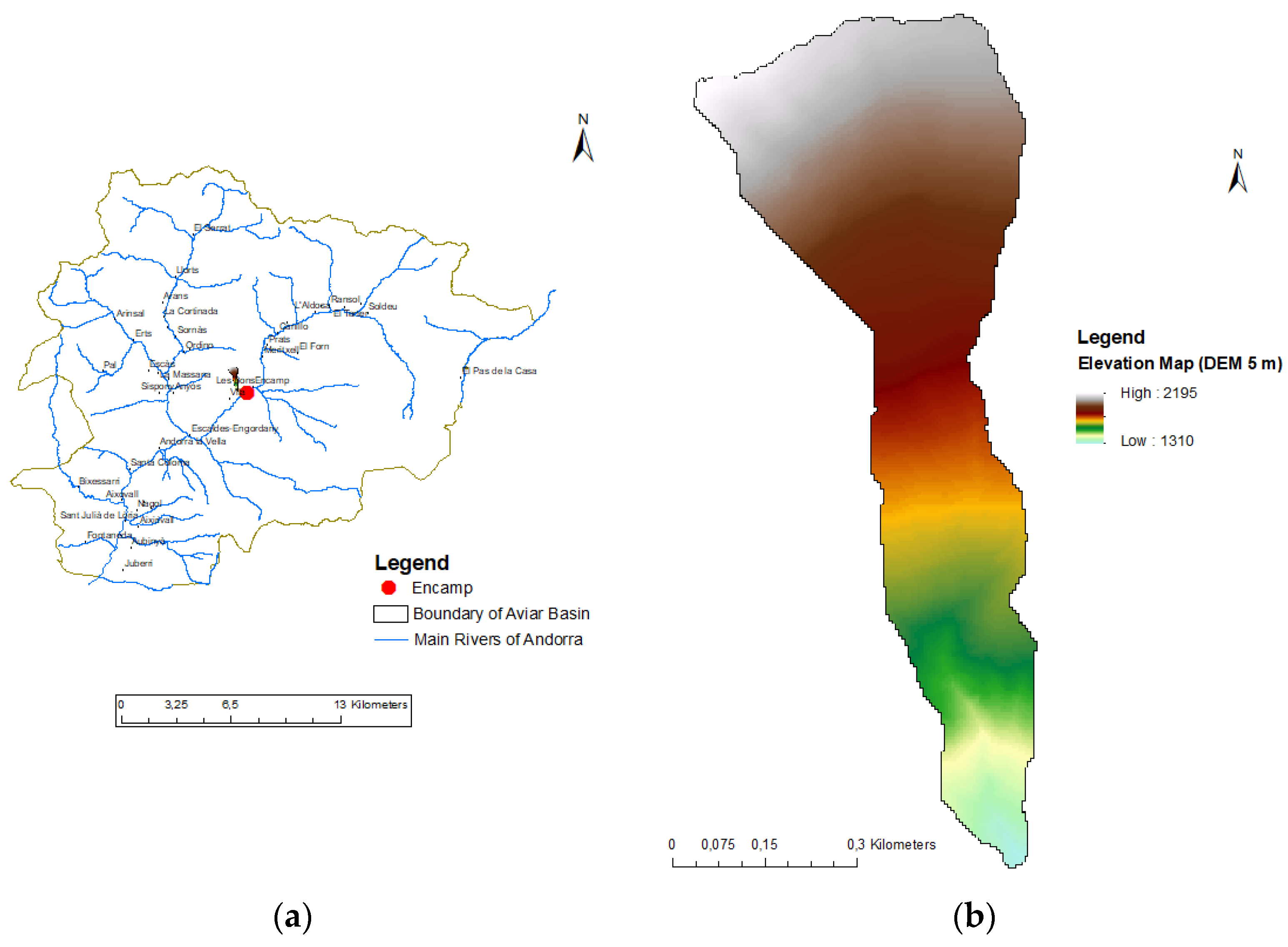
The study basin is located in the north hillside of the transverse valley of Encamp, a town located in Andorra, as shown in Figure 1a. Encamp (Andorra) has a mountainous Mediterranean-type climate, with a cold winter with heavy snowfalls, and a hot summer. Being a dry climate, the annual minimum average is −2 °C, and the maximum is 24 °C. Average annual rainfall ranges between 770 mm and 1100 mm. These precipitations are given in the form of rain in spring and autumn and mainly in the form of snow in winter.

Rainfall data used in this study comes from Roc de Sant Pere station, located 4 km away from our study area. It is the closest station and provides 6-minuterainfall data. In this study the rainfall events of 2012 were used and are shown in

Table 1. Events occurred in Encamp during 2012 [3].

Rainfall Event	Start	Stop	Total Rainfall (mm)	Duration (min)
Event 1	21 March 2012 11:00	21 March 2012 17:18	22.6	384
Event 2	21 March 2012 22:18	22 March 2012 03:00	14	288
Event 3	22 March 2012 12:00	22 March 2012 22:06	13.4	606
Event 4	23 March 2012 08:42	23 March 2012 16:12	20.2	456
Event 5	28 April 2012 14:54	29 April 2012 00:06	38.6	558
Event 6	19 May 2012 18:54	19 May 2012 22:18	16.2	210
Event 7	27 May 2012 10:42	27 May 2012 14:18	35	222
Event 8	2 June 2012 15:00	2 June 2012 18:18	16.4	204
Event 9	4 November 2012 9:48	4 November 2012 17:06	21.4	444
Event 10	26 November 2012 11:06	26 November 2012 19:54	22.6	534

.

The study basin, called Aviar Basin, is a peri-urban basin of 0.35 square kilometers. The elevation ranges are from 1.310 to 2.195 m above the sea level and the average slope of the basin is 51%.

In order to determine the surface soil composition of the basin, two samples of 30 cm depth were taken in Encamp to do a granulometric analysis using the sieving technique [3]. Analysis of the samples revealed that the surface soils are combined and mixed with big rock masses of Caradoc’s conglomerate, a very typical rock in the Pyrenees between the surface and a depth of 50–80 m. According to the Geological Map of Andorra [15], this material comes from the Ordovician epoch. The characteristics of sampled soils are summarized in

Table 2. Soil characteristics of the two samples [3].

Parameters	Sample 1	Sample 2
Fine	24.2%	33.2%
Sand	22.3%	13.3%
Gravel	53.5%	53.5%
D10 *	0.08 mm	0.08 mm
D50	2.55 mm	2.39 mm
D80	15.08 mm	21.33 mm
Structure type	Granular fine	Granular fine
Soil type based on USCS **	Sand (SM *** or SC ****)	Sand (SM *** or SC ****)

* D10: Particle diameter of 10% of soils classified as Fine; ** Unified Soil Classification System, ASTM D 2487–83 [16]; *** Silty sands, sand–silt mixtures; **** Clayey sands, sand–clay mixtures.

.

As in the rest of the Principality of Andorra, forests and shrubs cover a big part (2/5) of the extension in Encamp. Oaks predominate up to an elevation of 1200 m, with white pines being more common above that elevation. At elevations of 1600–1700 m, up to 2.200–2.300 m, black pines and alpine meadows predominate. The most common ground cover in the study area is forest and shrubs, as shown in Figure 2b.

3. Erosion Estimation Models Used

Soil erosion has been an important topic of study since the second quarter of the 20th century. Investigators have created different models throughout the years to determine the quantity of solid material eroded and/or deposited in a plot or in a basin. There are two main groups of erosion models: empirical models (USLE, RUSLE and MUSLE) and physically based models. In this study the physically based model used was KINEROS 2.

3.1. USLE

The Universal Soil Loss Equation (USLE) was developed in the USA around 1930 by the Soil Conservation Service of the US Department of Agriculture (USDA SCS), now known as the Natural Resources Conservation Service (NRCS). The USLE is the average of the annual loss of long-term soil (in metric tons per hectare and per year (ton/ha/year)), which is mathematically expressed as [17,18,19]:

$$A= R K\left(LS\right)C P$$

(1)

The parameters of R, K, LS, C, and P in Equation (1) are explained in detail, as follows.

3.1.1. Determination of Rainfall Erosivity Factor (R)

Rainfall-runoff erosivity factor is defined as the capacity of rain to produce erosion. It is also defined as the rainfall energy factor, and it is the product of total rainfall energy (E) and the maximum 30-min rainfall intensity (I₃₀) [1,13].

$$R={\displaystyle {\sum }_{i=1}^n{R}_i}={\displaystyle {\sum }_{i=1}^n{E}_c{I}_{30}}$$

(2)

where R_i is the rainfall energy factor of each rainfall, i is the number of rainfall events during the study year, E_c is the storm kinematic energy (in MJ/ha/year), and I₃₀ is the maximum intensity (in mm/h) during a 30-min rainfall interval [13,19].

First it is necessary to determine kinematic energy for every storm event and then obtain the R factor for this event. Total R factor will be the sum of R factors of each event [3,13,20].

3.1.2. Determination of Soil Erodibility Factor (K)

Soil erodibility factor (K) indicates the facility with which the soil suffers material losses from erosion. Wischmeier and Smith (1978) designed a nomograph and developed a regression algorithm to calculate K value. There is an alternative regression algorithm by Wischmeier et al. (1978) [1,13,20]:

$$K=\left[2.71\times {10}^{-6}{M}^{1.14}\left(12-a\right)\right]+4.2\times {10}^{-2}\left(b-2\right)+3.2\times {10}^{-2}\left(c-2\right)$$

(3)

where a is the organic matter by weight percentile, b is the structure number given as graph, c is the profile permeability class given as graph, and M is the texture representation factor, expressed as follows:

$$M=\left(100-clay\%\right)·\left(silt\%+fine sand\%\right)$$

(4)

K value is the average amount of annual soil lost per unit of the energy factor R of rainfall when the soil in issue is permanently bare, carved in favor of a 9% slope and 22.1 m in length [13]. Aggregate soil and dense vegetation cover reduce the vulnerability of soil to erosivity. Soil properties influencing the K factor include soil texture, organic matter, soil structure, and permeability of the soil profile [1]. K value was calculated using the results of granulometric analysis of soil samples made.

3.1.3. Determination of Length-Slope Factor (LS)

LS is the “Length-Slope” factor or “Topographical” factor, which is the influence of topography on the quantity of soil lost. It is important for two reasons:

• The angle of the slope modifies water permanency time that flows along basin surface.
• The length and the angle of the slope affects the kinetic energy that water that circulates on its surface will reach, therefore it will affect to erosive power.

There are several methods to obtain the LS factor, depending on the characteristics of the study basin. Wischmeier and Smith (1978) and Almorox et al. (1994) proposed the following Equation (5) for determining LS under conditions having a maximum slope of 20% and a maximum length of 300 m [13,18,19].

$$LS=L^{*}{S}^{*}={\left(\frac{X}{22.13}\right)}^m\left(\frac{0.43+0.3s+0.043s^2}{6.613}\right)$$

(5)

where L* is the length factor and S* is the slope factor, X is the hillside length (m) in its horizontal projection, m is the non-dimensional constant depending on an average slope s (%). The m values are 0.2 for s < 1%, 0.3 for 1% ≤ s <3%, 0.4 for 3% ≤ s < 5%, and 0.5 for 5% ≤ s.

The first formulation proposed by Wischmeier and Smith (1978) is limited for slopes lower than 20%. For conditions having slopes between 20~50% and lengths exceeding 300 m, Equation (6) is used to calculate the LS value [13].

$$LS=L^{*}{S}^{*}={\left(\frac{\lambda }{22.1}\right)}^{0.3}{\left(\frac{s}{9}\right)}^{1.3}$$

(6)

where λ is the hillside length (m) in its horizontal projection.

The global LS value is obtained by determining the weighted average of every segment of LS values. Refs. [13,20]

For slopes exceeding 50%, the USLE LS factor is out of range because these slopes typically have no soil. Therefore, determination of the LS value is not possible.

3.1.4. Determination of Crop Management Factor (C)

The term C in Equation (1) is the non-dimensional management factor related to vegetation cover and determines the relative effectiveness of soil and crop management systems in terms of preventing soil losses. Factor C is the product of three subfactors givenby different plots provided by Wischmeier and Smith (1978) [13]. The C factor of 0 represents a well-protected soil while the C factor of 1 is used to define the baseline condition with a clean-tilled, continuous fallow [1].

3.1.5. Determination of Conservation Practice Factor (P)

The term P in Equation (1) is the non-dimensional support practice factor, which reflects the relationship between the soil losses with a determined work practice: plow in terraces, in contour or crop in contour strips and irrigated furrows [1,13,19]. Soil losses under the USLE plowing conditions are given by Wischmeier and Smith (1978) [13]. USLE can only be used to calculate erosion by rain and cannot take into account snowmelt or rainfall on a frozen area.

3.2. RUSLE

In 1985, experts agreed to revise the USLE, to incorporate the results of new investigations and technologies. This revision was named the Revised Universal Soil Loss Equation (RUSLE). It incorporates important changes for estimating each parameter [20,21,22].

(1)

New maps of isolines to estimate the R factor.

(2)

The K factor now incorporates aspects related to frost processes.

(3)

The L and S parameters are now estimated according to new formulas because the influence of the slope length λ is increased, considering that increasing the length will increase the formation of streaks [20].

(4)

The C parameter includes new subfactors because RUSLE considers that erosion properties of soil change during the year depending on five new parameters: prior land use, canopy cover, surface cover, surface roughness and soil moisture [20].

(5)

The P parameter includes new considerations of agricultural practices taking into account crop slope [21].

While several authors have proposed different ways to calculate the factors of RUSLE, we have relied upon those proposed by Renard et al. (1997) [20].

As we can see in the conclusions, the RUSLE method is long and complex but if it is done with caution, better results are obtained from the RUSLE method than USLE method [3].

3.3. MUSLE

The Modified Universal Loss Equation (USLE Modified), was formulated differently from the USLE, in order to apply it to basins. Williams and others [19] modified the R factor used by the USLE in order to evaluate the volume Y of sediments produced by a single storm event (in tones, t) in a basin. Its expression is the following one:

$$Y=11.8{\left(Q q_p\right)}^{0.56}K C P \left(LS\right)$$

(7)

where Q is the runoff volume (m³) and q_p is the maximum instantaneous flow (m³/s).

The remaining factors of K, C, P, and LS in Equation (7) are the same as in the USLE formulation (Equation (1)).

3.4. Brief Introduction toKINEROS 2

KINEROS 2 is a dynamic, physically based, spatially distributed model that simulates a basin using a network of flat surfaces connected by channels. KINEROS 2 is open-code software that achieves a simulation of the hydrology and sedimentology that takes into account infiltration, interception, surface runoff, and erosion processes, principally for small urban or agricultural basins. KINEROS 2 calculates excess rainfall by adding amounts resulting from infiltration and interception processes to the amount of input rainfall. In addition, KINEROS 2 works in GIS base giving the user GIS tools to work with all raster information data needed: Digital Elevation Model, surface coverage map, etc., [4,18,23,24,25].

Infiltration is estimated using the Parlange 3-parameter model. Runoff is estimated using dynamic transport of the rainfall excess. KINEROS 2 uses the Kinematic Wave model for superficial flow transport in flat elements connected with channels [18].

The erosion/deposition rate is the combination of splash erosion and hydraulic erosion. Splash erosion is only considered in flat elements. Erosion by surface runoff is estimated taking into account the capacity of transport, calculated using the Engelund–Hansen Equation (8), developed in 1967 [4,18].

$$f^{\prime }\varphi =0,1·{\theta }^{2/5}$$

(8)

With:

$$f^{\prime }=\frac{2gSD}{v^2}$$

(9)

$$\varphi =q_t·{[{\gamma }_s·\left(\frac{{\gamma }_s-\gamma }{\gamma }\right)·g·d^3]}^{-1/2}$$

(10)

$$\theta =\frac{\tau }{\left({\gamma }_s-\gamma \right)·d}$$

(11)

where:

• $g$: Gravity.
• $S$: Energy slope.
• $D$: Waterdepth
• $v$: Average flow velocity.
• $q_t$: Total sediment discharge per width unit.
• ${\gamma }_s$: Specific weight of the sediment.
• $\gamma$: Specific weight of water.
• $d$: Average diameter of sediment particles.
• $\tau$: Tangential force along the riverbed.

Finally, sediment transport is calculated with the non-permanent flow continuity unidimensional equation.

3.4.1. Model Functioning

Basins are represented by spatially distributed elements: flat elements connected by channels up to basin outlet. KINEROS 2 model estimates hydrological losses taking into account the spatial variability. For that reason, KINEROS 2 considers rainfall, interception of soil vegetation cover, and infiltration.

3.4.2. Application to Aviar Basin

To delineate a basin, we must define the study basin boundary. First, the modeler has to populate the DEM (Digital Elevation Model) to avoid calculation errors. The second step is to define the direction and accumulation grid of flow. Both can be created either from GIS or from KINEROS 2.

The next step is basin discretization. KINEROS 2 creates flat elements using the calculated basin delineation. Basin discretization is based on a Contribution Area or CSA, which is defined by the KINEROS 2 user. This is the minimum area required to channel the water in a channel. The lower the CSA value, the higher the number of sub-basins. The KINEROS 2 default value for CSA is 2.5%. There are no recommendations about the value to select, although some considerations must be taken into account: small areas create more geometric components, and the CSA value may have to be adjusted to ensure that the results table for planes and streams does not result in null values appearing in the attribute tables [3].

3.4.3. Study Basin Parameterization

In order to conduct the calculations correctly, each element must be characterized with its geometry, flow length, vegetation cover and soil properties. KINEROS 2 parameterizes all components, giving them hydraulic and hydrology properties. This information cannot be extracted from the DEM. The Automated Geospatial Watershed Assessment (AGWA) uses a practical geometric relationship to calculate channel geometry as a function of the surface and background areas for each channel section.

Next, the soil and vegetation cover values must be parameterized, using the surface coverage map extracted from SIGMA and the soil sample analysis made. The hydrological properties of each type of cover and soil are included in the ‘LookUp’ table that we must attach so that KINEROS assigns each element the characteristic properties of its composition and coverage.

3.4.4. Study Basin Delineation

Using flow direction and flow accumulation grids previously calculated, the study basin can be defined, and an outlet point can be assigned. The outlet point coordination of the Aviar Basin is X = 5,317,165 m and Y = 26,540 m, according to the NTF (Nouvelle Triangulation de la France) projections. By completing all of the described steps, we delineated the Aviar Basin for use in the erosion study.

In Figure 3 we can see the delineator interface to show where the user has to input each grid previously calculated using KINEROS 2.

3.4.5. Study Basin Discretization

Following the steps described in Section 3.4.2 above, we defined the study basin characteristics (

Table 3. Detail value of study basin [3].

Characteristics	Value
Area	346,650 m2
Slope	0.51
Number of sub-basins (Planes)	57
Number of streams	23

and Figure 4) and the study basin area discretization scheme using KINEROS 2 (see Figure 5).

4. Discussion of Simulation Results

4.1. Hydrological Results of KINEROS 2

Once the basin was delineated, discretized in flat elements and channels, and we have these parameterized elements with vegetation and soils, we can introduce rainfall and run the model to obtain the simulation results. This model cannot be correctly validated without measuring the flow at the basin’s outlet for different rainfall events. The alternative is to pseudo-calibrate the KINEROS 2 model using another physically based model very similar to KINEROS 2, but already validated. This physical model (Zambrano et al., 2014) estimates erosion and sediment transportation in small peri-urban basins during singular events [4]. Hydrological results obtained from KINEROS 2 are compared with the results of the physically based model of Zambrano et al. (2014) [4]. All 2012 rainfall events are presented in comparative tables and graphs [3]. Comparing both models, the average difference is around 8%, which is adequate for the study case.

KINEROS 2 produces the graphic and table results for target area. It offers infiltration, runoff, peak flow, and solid material quantity for planes that discharge into channels and runoff into the basin outlet.

4.2. KINEROS 2 Sedimentological Results

The sedimentological model was validated using MUSLE results, due to the lack of measured data. In order to accomplish this, the study area average temperature was changed by applying a value of 2 °C. In addition, the erosive flow area decreased to 10% (the area composed of non-rocky material). Then, a new fine distribution was made using the investigations.

Table 4. Differences between calculated results using MUSLE and KINEROS 2 [3].

Rainfall Event	Total Rainfall (mm)	Duration (min)	KINEROS 2 Results (ton/ha)	MUSLE (ton/ha)	Differences %
Event 1	22.6	384	2.6	2.46	5.77
Event 2	14.0	288	0.033	0.030	18.18
Event 3	13.6	606	0	0	-
Event 4	20.2	456	0	0	-
Event 5	38.6	588	6.34	4.77	24.5
Event 6	16.2	210	1.93	1.72	11.4
Event 7	35.4	222	12.81	7.21	43.72
Event 8	16.8	204	7.45	5.06	32
Event 9	21.4	444	1.93	2.22	12.3
Event 10	22.6	534	1.12	1.77	36
TOTAL			34.21	25.157	26%
TOTAL (excluding Event 7)			21.20	17.957	15%

shows the differences between calculated results using MUSLE and KINEROS 2.

As we can see in the table above, results obtained with MUSLE and with KINEROS 2 are close in most of rainfall events in terms of absolute values. If we compare total eroded soil during the year, the difference of the final result is more significant. If we make the same final comparison excluding Event 7, final results are close between MUSLE and KINEROS 2 results, as we can see in previous table. The reason is that Event 7 could not be calibrated correctly. One unique rainfall event can spoil global annual erosion results.

KINEROS 2 offers an eroded solid material graphical representation. Figure 6 shows the graphical representation of eroded solid material from KINEROS 2 for Event 1 in the sub-basins and in the streams of Aviar Basin.

Once the annual eroded material quantity has been calculated by the four different methodologies, a comparison is made as shown in

Table 5. Sedimentological results for each method (including Event 7) [3].

Model	Erosion Amount (ton/ha/year)
USLE	20.674
RUSLE	24.443
MUSLE	25.497
KINEROS 2	34.213
Model of Zambrano et al.	26.750

.

Table 5 shows that there are differences between results of the different methods. The range of differences are between 1 ton/ha/year comparing RUSLE with MUSLE, and 13.5 tons/ha/year comparing USLE with KINEROS 2. This is mainly because the calibration of Event 7 cannot be completed adequately with KINEROS 2; however, we can get an idea of the eroded volume in the Aviar Basin, between 20–30 ton/ha/year. In conclusion, all results are compared and discussed. Differences between calculated erosion amounts for each method are shown in

Table 6. Differences between calculated erosion amounts for each method (including Event 7) [3].

MODEL	USLE	RUSLE	MUSLE	KINEROS 2	Zambrano et al. (2014)
USLE		15.42%	18.92%	39.5%	22.7%
RUSLE			4.13%	28.5%	8.6%
MUSLE				25.5%	4.7%
KINEROS 2					21.8%
Model of Zambrano et al.

.

Therefore, using one of these methods we can estimate the amount of eroded material to allow the implementation of adequate preventive measures to prevent the accumulation of sediments in sewer networks [10].

5. Conclusions

Erosion and sediment transport models offer an illustrative idea about natural processes. The development and utilization of computational tools that use numerical methods to solve mathematical formulations have increased our capacity to calculate results by allowing the incorporation of more parameters. These new physically based models have allowed the user to consider spatial and temporary variability of processes and parameters.

As it is demonstrated in this research, to have observed data of the modeled basin is essential to do an exact calibration. In absence of observed data, we have had to match the results of several models, which for some rainfall events can give differing results. Nevertheless, in the comparison of results, the soil loss estimation per hectare and per year are within the same order of magnitude. The first conclusion of this study is that we are approaching a valid result with KINEROS 2.

The RUSLE method is long and complex. Many researchers have participated in its formulation, contributing modifications to one or more of its parameters. To obtain a solid material mass value using RUSLE, it is necessary to calculate specific parameters, between intermediate and definitive calculations. However, if it is done with caution, better results are obtained from the RUSLE method than USLE method.

While the USLE method provides less realistic results than RUSLE, it is simpler to use. Furthermore, it was the first soil loss estimation formula, therefore it is now recommended to use more recent versions such as RUSLE or MUSLE. MUSLE obtains results that are closer to the results obtained from a physically based model, but it is necessary to obtain elsewhere the previous peak flow data for rainfall events.

KINEROS 2 is a semi-distributed model because it does not discretize the basin by cells but by sub-basins (composites by plane rectangular elements) that discharge into channels. If the user works with low resolution, average slopes will increase, enlarging flow velocity. In addition, sub-basins are represented by rectangular elements that shorten flow lengths, increasing runoff and flow times. In conclusion, without an optimal discretization, the calculated eroded sediment volume from the basin increases.

References

- Tiruwa, D.B.; Khanal, B.R.; Lamichhane, S.; Acharya, B.S. Soil erosion estimation using Geographic Information System (GIS) and Revised Universal Soil Loss Equation (RUSLE) in the Siwalik Hills of Nawalparasi, Nepal. J. Water Clim. Chang. 2021, 12, 1958–1974. [Google Scholar] [CrossRef]
- Armenise, E.; Simmons, R.W.; Ahn, S.J.; Garbout, A.; Doerr, S.H.; Mooney, S.J.; Sturrock, C.J.; Ritz, K. Soil seal development under simulated rainfall: Structural, physical and hydrological dynamics. J. Hydrol. 2018, 556, 211–219. [Google Scholar] [CrossRef] [PubMed]
- Fortuño Ibáñez, J. Erosion Study in Natural Basins Using Kineros 2. Master’s Thesis, Incheon National University, Incheon, Korea, 2017. [Google Scholar]
- Zambrano, J.D.; Gómez, M. Modelling of Erosion and Sediment Transport in Small Urban Areas Using a Single Event, Physical Model; Universidad Nacional de Colombia: Bogotá, Colombia; Flumen Institute, UniversitatPolitècnica de Catalunya: Barcelona, Spain, 2014. [Google Scholar]
- Cui, B.L.; Li, X.Y. Coastline change of the Yellow River estuary and its response to the sediment and runoff (1976–2005). Geomorphology 2011, 127, 32–40. [Google Scholar] [CrossRef]
- Blanckenburg, F. The control mechanisms of erosion and weathering at basin scale from cosmogenic nuclides in river sediment. Earth Planet. Sci. Lett. 2005, 237, 462–479. [Google Scholar] [CrossRef]
- Hugett, R.J. Fundamentals of Geomorphology; Routledge: London, UK, 2011. [Google Scholar]
- Nochet, E.; Poesen, J.; Rubio, J.L. Mound development as an interaction of individual plants with soil, water erosion and sedimentation processes on slopes. Earth Surf. Process. Landf. 2000, 25, 847–867. [Google Scholar]
- Dotterweich, M.; Rodzik, J.; Zgłobicki, W.; Schmitt, A.; Schmidtchen, G.; Bork, H.R. High resolution gully erosion and sedimentation processes, and land use changes since the Bronze Age and future trajectories in the Kazimierz Dolny area (Nałęczów Plateau, SE-Poland). Catena 2012, 95, 50–62. [Google Scholar] [CrossRef]
- Conesa, C. Los Diques de Retención en Cuencas de Régimen Torrencial: Diseño, Tipos y Funciones; Universidad de Murcia: Murcia, Spain, Nimbus N°13–14; 2004; pp. 125–142. ISSN 1139-1736. [Google Scholar]
- Alewell, C.; Borrelli, P.; Meusburger, K.; Panagos, P. Using the USLE: Chances, challenges and limitations of soil erosion modelling. Int. Soil Water Conserv. Res. 2019, 7, 203–225. [Google Scholar] [CrossRef]
- Salvany, M.C.; Marques, M.A.; Gallart, F. Modelos de Erosión de base física: Características y Utilidades. In Proceedings of the IV Reunión de Geomorfología, Sociedad Española de Geomorfología. A Coruña, Spain, 20 September 1996. [Google Scholar]
- Wischmeier, W.H.; Smith, D.D. Predicting Rainfall Erosion Losses: A Guide to Conservation Planning; Agriculture Handbook; U.S. Department of Agriculture: Washington, DC, USA, 1978; pp. 3–34.
- An, M.; Han, Y.; Xu, L.; Wang, X.; Ao, C.; Pang, D. KINEROS2-based simulation of total nitrogen loss on slopes under rainfall events. CATENA 2019, 177, 13–21. [Google Scholar] [CrossRef]
- Llopis, N.; Solé, J. Mapa Geológico de Andorra; Toponímia Según, M.C., Ed.; Instituto de Estudios Ilerdenses: Lleida, Spain, 1950. [Google Scholar]
- ASTM. Classification of Soils for Engineering Purposes; ASTM: West Conshohocken, PA, USA, 1985. [Google Scholar]
- Pham, T.G.; Degener, J.; Kappas, M. Integrated universal soil loss equation (USLE) and Geographical Information System (GIS) for soil erosion estimation in A Sap basin: Central Vietnam. Int. Soil Water Conserv. Res. 2018, 6, 99–110. [Google Scholar] [CrossRef]
- Goodrich, D.C.; Burns, I.S.; Unkrich, C.L.; Semmens, D.J.; Guertin, D.P.; Hernandez, M.; Yatheendradas, S.; Kennedy, J.R.; Levick, L.R. KINEROS2/AGWA: Model Use, Calibration, and Validation. Am. Soc. Agric. Biol. Eng. 2012, 55, 1561–1574. [Google Scholar] [CrossRef]
- Almorox Alonso, J.; Garcia, R.D.; Saa Requejo, A.; Álvarez, D.; Gasco Montes, J.M. Métodos de Estimación de la Erosión Hídrica; Editorial Agrícola Española: Madrid, Spain, 1994; pp. 62–125. [Google Scholar]
- Renard, K.G.; Foster, G.R.; Weessies, G.A.; McCool, D.K.; Yolder, D.C. Predicting Soil Erosion by Water: A Guide to Conservation Planning with the Revised Universal Soil Loss Equation (RUSLE); Agriculture Handbook; U.S. Department of Agriculture: Honolulu, HI, USA, 1997; pp. 19–227.
- Hateffard, F.; Mohammed, S.; Alsafadi, K.; Enaruvbe, G.O.; Heidari, A.; Abdo, H.G.; Rodrigo-Comino, J. CMIP5 climate projections and RUSLE-based soil erosion assessment in the central part of Iran. Sci. Rep. 2021, 11, 7273. [Google Scholar] [CrossRef] [PubMed]
- Elnashar, A.; Zeng, H.; Wu, B.; Fenta, A.A.; Nabil, M.; Duerler, R. Soil erosion assessment in the Blue Nile Basin driven by a novel RUSLE-GEE framework. Sci. Total Environ. 2021, 793, 148466. [Google Scholar] [CrossRef] [PubMed]
- Saran, S.; Sterk, G.; Aggarwal, S.P.; Dadhwal, V.K. Coupling Remote Sensing and GIS with KINEROS2 Model for Spatially Distributed Runoff Modeling in a Himalayan Watershed. J. Indian Soc. Remote Sens. 2021, 49, 1121–1139. [Google Scholar] [CrossRef]
- Smith, R.E.; Goodrich, D.C.; Quinton, J.N. Dynamic, distributed simulation of watershed erosion: The KINEROS2 and EUROSEM models. J. Soil Water Conserv. 1995, 50, 517–520. [Google Scholar]
- Korgaonkar, Y.; Meles, M.B.; Guertin, D.P.; Goodrich, D.C.; Goodrich, D.C.; Unkrich, C. Global sensitivity analysis of KINEROS2 hydrologic model parameters representing green infrastructure using the STAR-VARS framework. Environ. Model. Softw. 2020, 132, 104814. [Google Scholar] [CrossRef]