An Effective Simulation Scheme for Predicting the Aerodynamic Heat of a Scramjet-Propelled Vehicle

Abstract

Currently, aerothermal research into scramjet-propelled vehicles characterized by a wedge-shaped section is relatively sparse. Based on the Mach number, grid strategy, and numerical method, an effective simulation scheme for predicting the aerodynamic heat of a scramjet-propelled vehicle during flight is proposed in this paper. At different Mach numbers, the appropriate grid strategy and numerical method were determined by validation tests. Two-dimensional external flow field models based on wedge sections were established and, unlike in blunt bodies, the tests showed that at the high supersonic stage, the ideal cell Reynolds number should be no larger than 16. At the hypersonic stage, the ideal cell Reynolds number and aspect ratio of wall cells near the shock should be no larger than 40, and the AUSM+ flux type performs better than Roe’s FDS flux type at the above stages. The aerothermal prediction indicates that during a flight time of about 34 s, the temperature change reaches about 1913.35 °C, and the maximum average temperature change rate reaches 115 °C/s.

1. Introduction

Aerodynamic heat prediction plays an important role in the design and optimization of hypersonic vehicles [1,2]. In general, there are three technical approaches to aerodynamic heat prediction: the engineering estimation [3], the wind tunnel experiment [4], and computational fluid dynamics (CFD) [5,6]. With the development of computer technology, CFD has made great progress; its results offer higher accuracy than engineering estimation, and, unlike the wind tunnel experiment, its simulation ability can cover the entire flight trajectory. The CFD technology has become an indispensable means in the study of aerothermal predictions. Its results are influenced by many factors, such as Mach number, gird strategy, and numerical methods, which include turbulence models, upwind scheme, limiter, and so on. Domestic and foreign scholars have carried out research into these factors. The aerodynamic characteristics of different Mach numbers are different, and the corresponding grid strategy and numerical method are also different [7]. In terms of grid strategy, the height of the first layer of wall cells has a great influence on the numerical calculation results, and the mesh needs to be adjusted several times according to the CFD results, which is a time-consuming part of the CFD process. Ref. [8] discusses the effect of the grid on aerothermal prediction by taking an external flow field simulation model based on a blunt body as an example. The results show that the deviation of the results could reach more than 20% when the Reynolds number of the wall grid is doubled while other conditions are unchanged. Ref. [9] considers the effect of cell Reynolds numbers on aerothermal prediction by applying a cylinder as an example. The results show that it is necessary to keep the cell Reynolds number less than 10 in the aerothermal calculation, and Refs. [10,11] presents similar research cases. Ref. [12] shows that the property of shock stability influences the accuracy of heating prediction. Ref. [13] reveals that the aspect ratio of wall cells near the shock is a major factor and Ref. [14] suggests that the aspect ratio of wall cells near the shock should be larger than six for predicting hypersonic heating, taking a blunt body and a blunt cone as examples. The experimental data of X33, which is a reusable reentry hypersonic vehicle, are used to validate the above conclusions. In terms of the numerical method, turbulence is a difficult problem in flows and the current simulation equations for turbulence include Reynolds Averaged Navier-Stokes (RANS), Large Eddy, Separated Eddy, and Direct Numerical Simulation (DNS), etc. Considering the limitations of robustness and computational efficiency, RANS is still the main turbulence simulation method adopted at present [15]. When there are discontinuities in flows, the artificial viscosity, which can affect the calculation accuracy, is usually added to the central scheme to suppress oscillations. Therefore, varieties of upwind schemes have gradually become the mainstream approach to numerical calculation. In addition, the limiter is applied to limit the difference gradient to avoid oscillations. Ref. [16] discusses the calculation accuracy of AUSM+, Roe’s FDS, and FVS by taking the flow around a cylinder and a blunt as examples. The results show that the calculation accuracy of these three upwind schemes is better than that of the central difference scheme, and the numerical results of AUSM+ and Roe’s FDS are closer to the experimental data. Ref. [17] adopts Minmod, van leer, and osher-c limiters to simulate the external flow field of a blunt. The results indicate that the maximum heat flow value and heat distribution characteristics obtained by the Minmod limiter are better than the other two limiters.

In current research, the reusable reentry vehicle is the main research object of aerothermal prediction. The external flow field model for simulation is primarily based on blunt bodies, and the initial conditions of freestream are usually selected from a certain stage in the flight path, such as the hypersonic stage. However for the scramjet-propelled vehicle with a wedge section as its characteristic component, research on the aerodynamics heat prediction in the flight path is relatively sparse. In this study, a 2D external flow field model was built based on a wedge section, and an aerothermal prediction was performed for its flight path is performed. This approach can further enrich and improve aerothermal research into hypersonic vehicles.

This manuscript is organized as follows. In the second section, we briefly overview the flight path of a scramjet-propelled vehicle and the numerical procedures applied in the CFD. Next, according to the Mach number, the flight trajectory of the scramjet-propelled vehicle is divided into different stages, and the determination of the appropriate grid strategy and numerical method through validation tests is presented in the third section. Based on the simulation parameters confirmed in these sections, an effective simulation scheme for the scramjet-propelled vehicle is then proposed, and the prediction of the aerodynamic heat during the flight is discussed in in the fourth section. The last section presents our conclusions.

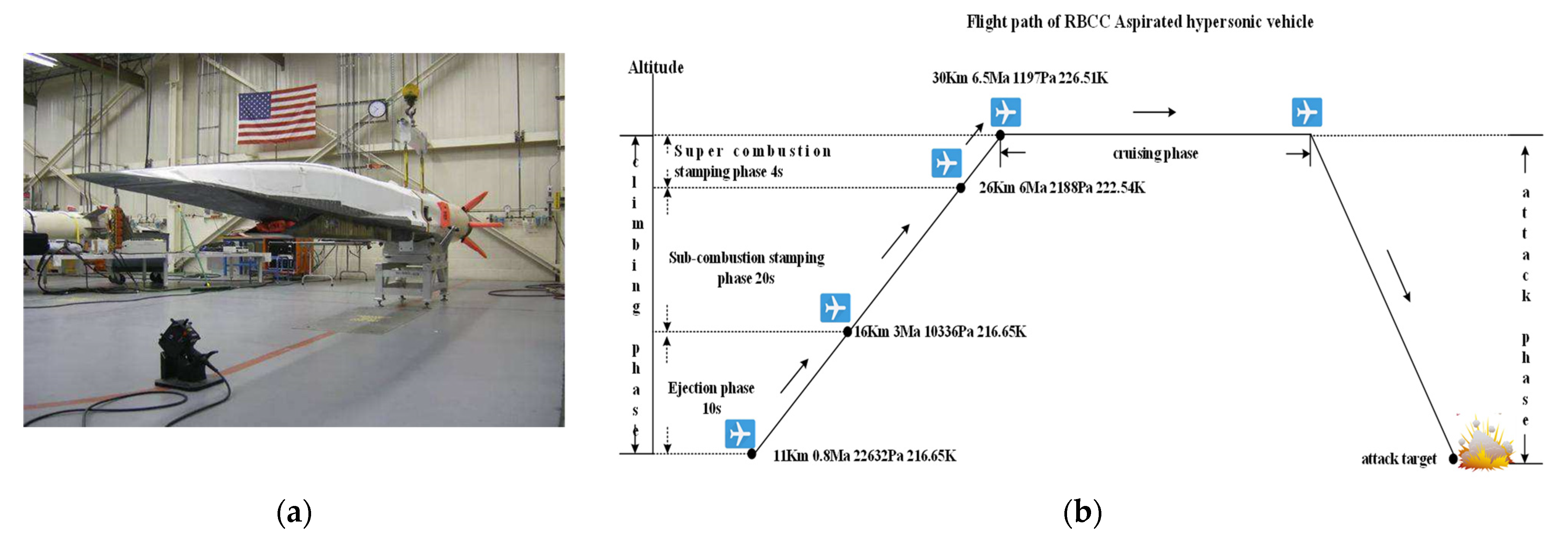
2. Flight Path of Scramjet-Propelled Vehicle and Numerical Procedures

Rocket-based combined cycle (RBCC) is the ideal power system for future scramjet-propelled vehicles and single-stage re-use vehicles. To minimize wave resistance during flight, RBCC vehicles tend to have a pointed head with a slender fuselage, and the typical part of RBCC vehicles is a wedge-shaped section. The X51A vehicle and its flight path are as shown in Figure 1a,b [18]. The flight path consists of a climbing phase, cruising phase, and attack phase, and the climbing phase also includes an ejection phase, a sub-combustion stamping phase, and a super-combustion stamping phase. During the climbing phase, the flight speed of the vehicle rapidly increases, and it is a phase of complex temperature changes. In the cruising phase, the vehicle keeps a constant altitude and speed and the flight distance accounts for about 90% of the total range; it could be viewed as a steady-state phase. These two phases are the main phases of the flight path, and the simulation scheme for aerodynamic heat prediction is proposed covering these two phases in this paper. After arriving at the target airspace, the vehicle enters the attack phase, in which it shifts down and attacks the target accurately.

According to the different Mach numbers, the vehicle is in different external flow field environments [7,19]. At the transonic speed stage (when the Mach number is between 0.6 and 1), compressibility effects such as flow choking becoming important. At the supersonic speed stage (Mach number between 1 and 3), depending on the specific shape of the aircraft, a shock wave may be produced in the airflow. At the high supersonic (when the Mach number is between 3 and 5) and hypersonic speed stage (when the Mach number is bigger than 5), aerodynamic heating becomes very important. The flight path of the RBCC scramjet-propelled vehicle spans all of the above stages; therefore, a specific piecewise analysis is needed. According to the Mach number of the flight path, the simulation scheme is divided into four stages. To ensure the reliability of the prediction results, the simulation parameters should be confirmed by validation tests at each stage.

For flows involving compressibility and heat transfer, three conservation equations for mass, momentum, and energy need to be solved. When the flow is turbulent, additional transport equations are also solved, adopting the one-equation RANS Spalart-Allmaras model, which is the most widely applied [20], and the two-equation RANS SST k-omega turbulence model [21]. The control-volume-based technique is used to discretize the above equations. Firstly, the external flow field model is divided into discrete control volumes using a computational grid. Secondly, the integration of equations on the individual control volumes to algebraic equations for the discrete dependent variables and conserved scalars is accomplished using an upwind scheme. Next, the above-discretized equations are linearized, and the resultant linear equation system is solved to yield variables. Two numerical solvers, a pressure-based solver and a density-based solver, were applied in this study. More details about these equations and the finite volume method could be found in Ref. [22].

3. Validation Tests

3.1. Transonic Stage

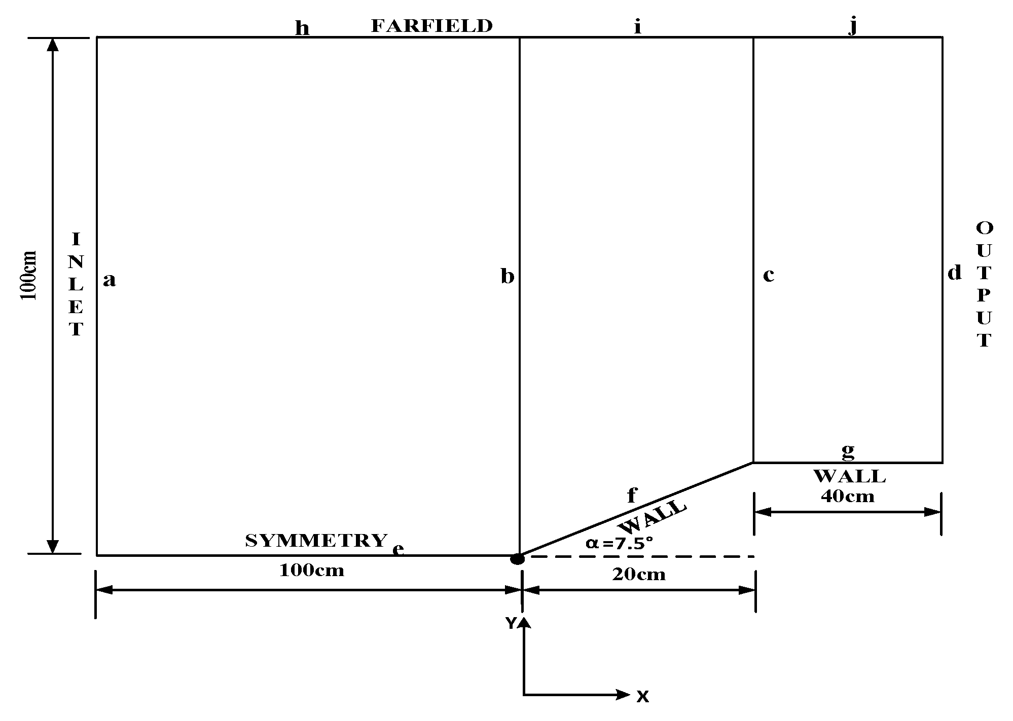
3.1.1. Grid Strategy

The experimental data in Ref. [23] are used to validate the simulation parameters at this stage, and the simulation external flow field model is as shown in Figure 2. The bold black dot is the (0,0) point of the coordinate system. Line f is the wedge section, line g is the flat plate.

Turbulent flows are affected by the presence of walls; therefore, the accurate representation of the flow in the near-wall region determines the successful prediction of wall-bounded turbulent flows, and it is necessary to ensure the first layer cells of the boundary layer are in the sub-viscosity layer. The calculation of the height of the first layer cells of the boundary layer begins with the flow Reynolds number (R_e):

$$R_e=\frac{\rho UL}{\mu }$$

(1)

where L is the characteristic length of the wedge, μ is the dynamic viscosity of the air, $\rho$ is the air density, and U is the velocity of freestream. Considering that the simulation model is wedge-shaped, an empirical correlation formulation to estimate the skin friction coefficient ($C_f$) is adopted, which is for the fully developed turbulent flow over a flat plate:

$$C_f=\left[2{\log }_{10}(R_e\right)-0.65{]}^{-2.3}$$

(2)

Having computed the skin friction coefficient, the wall shear stress (${\tau }_W$) is calculated:

$${\tau }_W=\frac{1}{2}\rho U^2{C}_f$$

(3)

After that, we can calculate the friction velocity ($u_{\tau }$) from the wall shear stress (${\tau }_W$):

$$u_{\tau }={(\frac{{\tau }_W}{\rho })}^{0.5}$$

(4)

The equation for $y^{+}$ is:

$$y^{+}=\frac{\rho y_P{u}_{\tau }}{\mu }$$

(5)

Therefore, the height of the wall-adjacent cell centroid from the wall ($y_P$) is:

$$y_P=\frac{y^{+}\mu }{u_{\tau }\rho }$$

(6)

Finally, the first height of the boundary layer cell ($y_H$) is double $y_P$:

$$y_H=2y_P$$

(7)

The result of the first height of the boundary layer cell is an estimate and needs to be updated using information from the CFD analysis. In addition to calculating the $y_H$, the growth ratio (r) normal to the wall and inflation layers (N) may also be required by mesh generation, which allows the layers to inflate normally to the wall. For aerodynamic flows using RANS turbulence modeling, CFD often aims for N = 15–30 through the thickness of the boundary layer. By adopting this criterion, we can calculate r normally to the wall, which is started by applying the formulation to estimate the boundary layer thickness, where $R_e$ is bigger than 5 × 10⁵:

$$\delta =\frac{0.38L}{R_e{}^{0.2}}$$

(8)

For a given number of r and N, we can calculate the total thickness of the inflation layers. Next, we match this to the boundary layer thickness $\delta$ to allow the inflation layers to cover the boundary layer thickness. Assume that the inflation layer has two layers, then the total thickness ($y_T$) is:

$$y_T=y_H+y_{H}r$$

(9)

Similarly, the total thickness of four inflation layers is:

$$y_T=y_H+y_{H}r+y_H{r}^2+y_H{r}^3$$

(10)

Therefore, the total thickness of N inflation layers is:

$$y_T={\displaystyle \sum }_{i=0}^{N-1}{y}_H{r}^i$$

(11)

Equation (11) is the formula of a geometric series, which could be rewritten using the identity for convenience:

$${\displaystyle \sum }_{i=0}^{N-1}{y}_H{r}^i=y_H\frac{1-r^N}{1-r}$$

(12)

Hence, the total thickness of the inflation layer is:

$$y_T=y_H\frac{1-r^N}{1-r}$$

(13)

Now, the error between the total thickness of the inflation layer $y_T$ and the thickness of the boundary layer $\delta$ is:

$$e=y_H\frac{1-r^N}{1-r}-\delta$$

(14)

Equation (14) is a function of the growth ratio r and we need to find a value of r to make the error equal to 0, which is the total height of the inflation layer equal to the boundary layer thickness. The Newton-Raphson root-finding algorithm is adopted, and once the algorithm has converged, the solution r is the maximum growth ratio. Because, in mesh generators, the r is always greater than 1 and less than 2, the initial guess of 1 and 2 could be used to bound the root-finding algorithm to accelerate the convergence.

Three different Mach numbers, 0.768, 0.817. and 0.86 were applied, respectively, in the validation tests at the subsonic stage. The static temperature of freestream T was 300 K and the dynamic viscosity $\mu$ was 1.7894 × 10⁻⁵ Pa·s; the density of air was ideal-gas, the specific heat at a constant air pressure was 1006.43 j/kg-k, and the characteristic length c was 0.59696 m. Initially, $y^{+}$ was 5 to ensure the first layer cells of the boundary layer were in the sub-viscosity layer, and $y_H$ was 1.53 × 10⁻⁵, according to Equations (1)–(7). Next, the CFD analysis showed that the maximum value of $y^{+}$ at the WALL surface reached 6.5. The simulation tests showed that the $y^{+}$ value of 1 could guarantee that the first layer cells of the boundary layer are in the sub-viscosity layer during the simulation process. The turbulent viscosity ratio (TVR) was adopted to evaluate whether the boundary layer profile was captured well. Figure 3 shows the corresponding plots of the TVR for the mesh with $y^{+}$ = 1 and N = 20, since the $y^{+}$ value is 1, which means presence within the laminar sub-layer, and absence of turbulent viscosity. As the mesh moved through the buffer region and into the logarithmic region, the TVR value increased, and the maximum value occurred near the middle of the boundary layer. Subsequently, the turbulence gradually dissipated as the mesh approached the free stream condition, which was expected. Therefore, the values of $y^{+}$ and N were sufficient, so we could calculate the maximum growth ratio r by Equation (14). The first layer height $y_H$ and the maximum growth ratio were (1.49 × 10⁻⁶, 1.42), (1.38 × 10⁻⁶, 1.42) and (8.42 × 10⁻⁶, 1.34) respectively.

To determine the best domain size, computational region analysis was performed. For this purpose, three sizes were chosen, as shown in Figure 4a [24]. The INLET boundary contained line a, the OUTPUT boundary contained line d, the FARDIELD boundary contained lines h, i, and j, the SYMMETRY boundary contained line e, and the WALL boundary contained lines f and g. Figure 4b offers a close view of the grids near the WALL region. Taking the numerical simulation adopting freestream Mach number of 0.768 and the Spalart-Allmaras model as an example, the values of the local Mach number m, the pressure coefficient (c_p), and the temperature are as shown in

Table 1. Computational domain independency study of three levels of sizes with error ratios.

Computational Domains	x/c (m, cp, Temperature and Error Ratio)
	0			0.2			0.4			0.6			0.8			1
6	0.3745	0.6719	308.5	0.59013	0.4052	290.7	0.63756	0.3451	290.1	0.67321	0.2939	284.4	0.71826	0.2351	286.7	0.8773	0.00459	287.7
	15.49%	12.54	/	14.25%	13.09%	/	13.52%	11.68%	/	13.29%	11.95%	/	13.8%	12.13%	/	10.49%	10.4%	/
8	0.3793	0.6819	321.5	0.59774	0.4112	302.7	0.64396	0.3497	302.8	0.68116	0.2971	300.7	0.72441	0.239	301.8	0.886	0.00465	302.1
	14.41	11.24	/	13.15%	11.81%	/	12.65%	10.5%	/	12.26%	10.99%	/	13.06%	10.67%	/	9.58%	9.23%	/
12	0.3779	0.6769	329.2	0.59644	0.4097	311.3	0.64085	0.3477	309.1	0.67843	0.2964	310.2	0.7211	0.2371	310.2	0.882	0.00463	311.2
	14.72	11.89	/	13.34%	12.13%	/	13.07%	11.01%	/	12.62%	11.2%	/	13.46%	11.38%	/	10.02%	9.62%	/

, where x is the X-axis location, and the computational domain with 8c was chosen for low errors. Further, to be sure of grid independency, three levels of different mesh were applied. As can be seen in

Table 2. Grid independency study of three levels of different mesh with error ratios.

Mesh (Cells)	x/c (m, cp, Temperature and Error Ratio)
	0			0.2			0.4			0.6			0.8			1
210,000	0.3793	0.6819	321.5	0.59774	0.4112	302.7	0.64396	0.3497	302.8	0.68116	0.2971	300.7	0.72441	0.239	301.8	0.886	0.00465	302.1
	14.41%	11.24%	/	13.15%	11.8%	/	12.65%	10.5%	/	12.26%	10.99%	/	13.06%	10.67%	/	9.58%	9.23%	/
480,000	0.4025	0.7032	330.9	0.62447	0.4262	312.3	0.67889	0.3636	312.3	0.71274	0.3091	310.6	0.75994	0.2481	310.9	0.915	0.00481	311.7
	9.17%	8.46%	/	9.26%	8.59%	/	7.91%	6.95%	/	8.2%	7.39%	/	8.79%	7.27%	/	6.7%	6.10%	/
680,000	0.3978	0.6919	331.2	0.62047	0.4198	312.7	0.66488	0.3591	313.1	0.70963	0.3041	308.2	0.743	0.2438	310.2	0.901	0.00475	312.5
	10.23%	9.93%	/	9.84%	9.96%	/	9.81%	8.1%	/	8.60%	8.89%	/	10.78%	8.87%	/	8.06%	7.27%	/

, it is clear that the values of m at 480,000 were better; therefore, the mesh with 480,000 cells was selected.

3.1.2. Numerical Method

At the transonic stage, the pressure-based solver was used with a coupled algorithm [25]. The second-order upwind interpolation scheme was selected for the density [26]. The gradients were computed according to the least-squares cell-based method. For preventing spurious oscillations, a gradient limiter was adopted, which used the Minmod function [17] to limit and clip the reconstructed solution overshoots and undershoots on the cell faces. The second-order scheme was used for interpolating the pressure values at the faces, which reconstructed the face pressure using a central differencing scheme. The validation parameters of the convergence numerical results were as shown in

Table 3. Validation parameters of convergence results at the transonic stage.

Validation Parameters
Solver	Pressure-based with coupled algorithm	Pressure-based with coupled algorithm
Turbulence Models	SST k-omega	Spalart-Allmaras
Materials	Density: Ideal-gas	Density: Ideal-gas
	Viscosity: 1.7894 × 10−5 Pa·s	Viscosity: 1.7894 × 10−5 Pa·s
	Cp (j/kg-k): 1006.43	Cp (j/kg-k): 1006.43
Initial conditions	Mach number: 0.768/0.817/0.86	Mach number: 0.768/0.817/0.86
	Static temperature: 300 K	Static temperature: 300 K
Boundary conditions	INPUT: pressure far field	INPUT: pressure far field
	FARFIELD: pressure far field	FARFIELD: pressure far field
	OUTPUT: pressure outlet	OUTPUT: pressure outlet
	SYMMETRY: symmetry	SYMMETRY: symmetry
	WALL: no-slip, isothermal	WALL: no-slip, isothermal

.

3.1.3. Simulation Parameters

Figure 5 demonstrates the distributions of m under three different Mach numbers of freestream $M$, where the X-axis was the ratio between x and c and the Y-axis was the value of m. EXP represents the experimental data, SST and SA represent the simulation results based on SST k-omega and Spalart-Allmaras, respectively. The overall tracking effect of the simulation data on the experiment data was good. At $M$ = 0.768, the average error rate of SST k-omega was 9.69%, and that of Spalart-Allmaras was 8.34%. The variance of SST k-omega error was 0.000368, and that of Spalart-Allmaras is 0.000122. At $M$ = 0.817, the average error rate of SST k-omega was 9.52%, and that of Spalart-Allmaras was 8.18%. The variance of SST k-omega error was 0.00035, and that of Spalart-Allmaras was 0.000152. At $M$ = 0.86, the average error rate of SST k-omega was 10.14%, and that of Spalart-Allmaras was 8.52%. The variance of SST k-omega error was 0.000359, and that of Spalart-Allmaras was 0.000284. The total mean error rates were 9.78% for SST and 8.35% for Spalart-Allmaras. In general, the trend of the simulation results was in good agreement with the experimental data, and of the two models, the Spalart-Allmaras simulation results were better than those of SST k-omega at the transonic stage.

In conclusion, the mesh with the value of $y^{+}$ as 1, = the turbulence model applying Spalart-Allmaras and the pressure-based solver, adopting a coupled algorithm, is preferred at the transonic stage.

3.2. Supersonic Stage

3.2.1. Grid Strategy

The experimental data in Ref. [27] were used to validate the simulation parameters at this stage. Given the existence of the shock wave in the airflow, the value of the shock wave angle was estimated firstly. The Mach number $M$ was 2.85 and the wedge angle α is 30°, which meets the Equation (15), where $\gamma$ = 1.4:

$$\alpha <\frac{4}{3\sqrt{3}\left(\gamma +1\right)}\frac{{(M^2-1)}^{\raisebox{1ex}{$3$}\!\left/ \!\raisebox{-1ex}{$2$}\right.}}{M^2}$$

(15)

The shock angle s was 54°, which was calculated by Equation (16):

$$\cot \alpha =\tan s[\frac{\left(r+1\right)M^2}{2(M^2{(\sin s)}^2-1}-1]$$

(16)

Next, we established and divided the external flow field model for the simulation, as shown in Figure 6. The bold black dot is the (0,0) point of the coordinate system. Lines o and q are the flat plate and line p is the wedge section. The bold black square point is the origin of the wedge section.

At the supersonic stage, the total temperature of the freestream T_t was 270 K and the total pressure of the freestream $p_t$ was 1.7 atm. The static temperature of the freestream T was calculated by Equation (17) and T was 102.88 K:

$$\frac{T_t}{T}=1+\frac{\gamma -1}{2}{M}^2$$

(17)

The static pressure of the freestream p was calculated by Equation (18) and p was 5881 Pa:

$$\frac{p_t}{p}={(1+\frac{\gamma -1}{2}{M}^2)}^{\frac{\gamma }{\gamma -1}}$$

(18)

The speed of sound $C_{air}$ was calculated by Equation (19) and $C_{air}$ was 203.36348 m/s:

$$C_{air}=20.05\sqrt{T}$$

(19)

The Mach number $M$ was 2.85 and the velocity of the freestream U was 579.5859 m/s. The corresponding unit Reynolds number of the freestream was 18 × 10⁶, the characteristic length L was 1.08 m, the density of air was ideal-gas, the specific heat at constant air pressure was 1006.43 j/kg-k, and the viscosity adopted three-coefficient Sutherland Law. Initially, we referred to the value of $y^{+}$ at the transonic stage to estimate $y_H$ 3.25 × 10⁻⁶, while the test results showed that the maximum $y^{+}$ of the wall surface exceeded 1 during the simulation. As described in the previous section, considering the maximum $y^{+}$ of wall surface during the CFD simulation and the boundary layer profile through TVR, the $y^{+}$ value was 0.8 and the $y_H$ value was 2.5 × 10⁻⁶.

To determine the best domain size, a computational region analysis is performed. For this purpose, three sizes were chosen, as shown in Figure 7a [24]. The INLET boundary contains line a and h, the OUTPUT boundary contains lines d and k, the FARDIELD boundary contains lines l, m, and n and the WALL boundary contains lines o, p, and q. Because of the shock wave, in order to obtain more accurate results, more attention was needed for the grids near the shock wave regions. Figure 7b demonstrates the close view of the grids near the shock wave region. Taking the SST k-omega model as an example, the values of the ratio between the wall surface pressure p and $p_t$, and temperature are as shown in

Table 4. Computational domain independency study of three levels of sizes with error ratios.

Computational Domain	x (m) (p/pt, Temperature and Error Ratio)
	0		0.02		0.04		0.06		0.08
6c	0.0873	241.887	0.1088	239.475	0.1372	242.097	0.0451	242.643	0.0348	243.842
	10.33%	/	10.78%	/	9.68%	/	12.1%	/	11.26%	/
8c	0.0861	252.149	0.1103	252.941	0.1396	253.461	0.0443	254.013	0.0353	254.314
	8.81%	/	9.55%	/	8.1%	/	10.11%	/	9.98%	/
12c	0.0868	259.411	0.1098	258.115	0.1389	257.329	0.0446	259.227	0.0351	257.669
	9.7%	/	9.96%	/	8.56%	/	10.86%	/	10.49%	/

, where x is the distance to the origin point of the wedge section, and the computational domain with 8c was chosen for low ratio errors. Next, three levels of different mesh were applied to ensure grid independency. From

Table 5. Grid independency study of three levels of different mesh with error ratios.

Mesh (Cells)	x (m) (p/pt, Temperature and Error Ratio)
	0		0.02		0.04		0.06		0.08
270,000	0.0861	252.149	0.1103	252.941	0.1396	253.461	0.0443	254.013	0.0353	254.314
	8.81%	/	9.55%	/	8.10%	/	10.11%	/	9.98%	/
520,000	0.0850	262.052	0.1118	262.631	0.1412	263.803	0.0439	264.211	0.0358	264.702
	7.44%	/	8.28%	/	7.08%	/	9.33%	/	8.83%	/
720,000	0.0853	264.043	0.1117	260.574	0.1405	264.887	0.0441	262.059	0.0356	265.413
	7.80%	/	8.40%	/	7.51%	/	9.61%	/	9.22%	/

, the mesh with 520,000 cells was applied at this stage.

3.2.2. Numerical Method

At the supersonic stage, the numerical method is similar to the transonic stage. The validation parameters of the convergence numerical results are shown in

Table 6. Validation parameters of convergence results at the supersonic stage.

Validation Parameters
Solver	Pressure-based with coupled algorithm	Pressure-based with coupled algorithm
Models	SST k-omega	Spalart-Allmaras
Materials	Density: Ideal-gas	Density: Ideal-gas
	Viscosity: Sutherland law	Viscosity: Sutherland law
	Cp (j/kg-k): 1006.43	Cp (j/kg-k): 1006.43
Initial conditions	Mach number: 2.85	Mach number: 2.85
	Static pressure: 5881 Pa	Static pressure: 5881 Pa
	Static Temperature: 102.88 K	Static Temperature: 102.88 K
Boundary conditions	INPUT: pressure far field	INPUT: pressure far field
	FARFIELD: pressure far field	FARFIELD: pressure far field
	OUTPUT: pressure outlet	OUTPUT: pressure outlet
	WALL: no-slip, isothermal, 300 K	WALL: no-slip, isothermal, 300 K

.

3.2.3. Simulation Parameters

Figure 8 shows the wall surface pressure distributions from the experiment and the simulation, where the X-axis x is the distance to the original point of the wedge section and the Y-axis is the ratio between the wall surface pressure and the total pressure of the freestream. The overall tracking effect of the simulation data on the experiment data was acceptable. The simulation errors of the two models were very close at the upper stream of the wedge section. At the wedge section, where x was bigger than 0, the mean error rate of SST k-omega data was 4.76%, and that of Spalart-Allmaras was 5.19%. The variance of SST k-omega simulation error was 0.001043, and that of Spalart-Allmaras was 0.003091. Figure 9 indicates the density profiles at x = 0 from the experiment and the simulation, the X-axis is the ratio between local density and the freestream density, and the Y-axis is the y location. The average error rate of the SST k-omega data was 7.92%, and that of Spalart-Allmaras was 10.04%. The variance of the SST k-omega simulation error was 0.00307, and that of Spalart-Allmaras was 0.003417. In general, the trend of the simulation results was in good agreement with the experimental data, and the SST k-omega simulation results were better than those of Spalart-Allmaras at the supersonic stage.

3.3. High Supersonic Stage

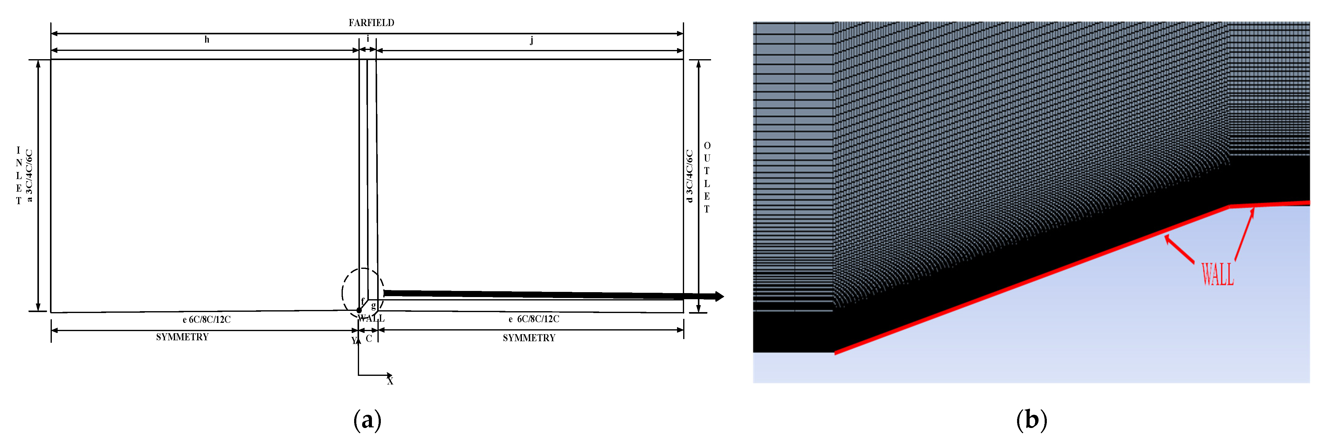
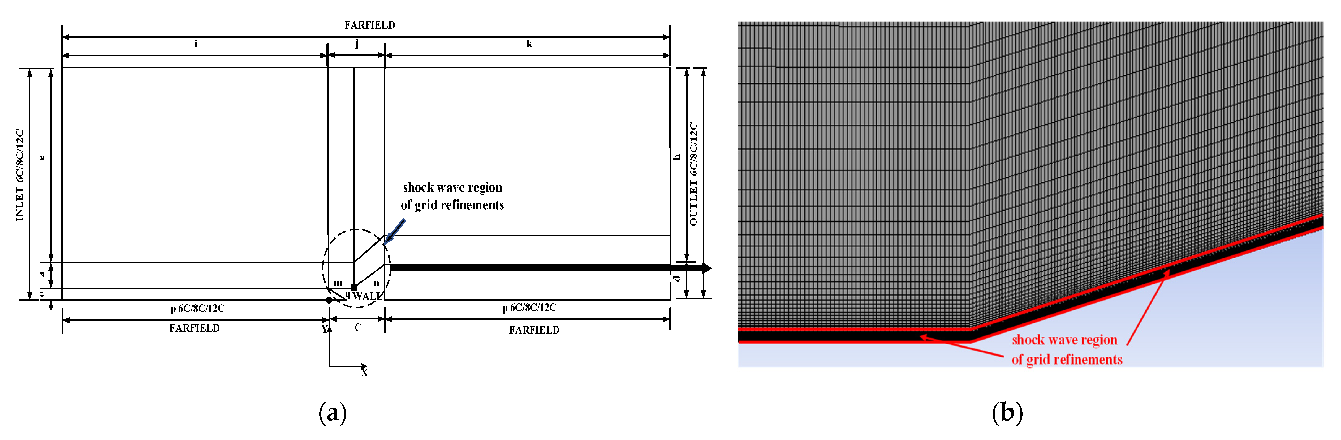
3.3.1. Grid Strategy

The experimental data in Ref. [28] were used to validate the simulation parameters at this stage. The Mach number M was 5 and the wedge angle α was 15°. The shock angle s was 24.32°, which was calculated by Equation (16). Next, we established and divided the external flow field model for the simulation, as shown in Figure 10. The bold black dot is the (0,0) point of the coordinate system. Line m is the flat plate and line n is the wedge section. The bold black square point is the origin of the wedge section. L is the distance between the flat plate’s leading edge and the wedge section origin, which was 0.25 m.

At the high supersonic stage, the total temperature of the freestream $T_t$ was 475 K and the total pressure of the freestream $p_t$ was 4.5 × 10⁵ Pa. The thermal conditions at the wall were $T_w$ = 100 K leading to a ratio $T_W/T_r$ = 0.24 and $T_w$ = 290 K leading to a ratio $T_W/T_r$ = 0.72, where $T_r$ is the recovery temperature. The static temperature of the freestream T was calculated by Equation (17), and T was 79.17 K; the static pressure of the freestream p was calculated by Equation (18), and p is 850.5173 Pa; the speed of sound $C_{air}$ was calculated by Equation (19), and $C_{air}$ was 178.3999 m/s. The Mach number $M$ was 5 and the velocity of the freestream U was 891.99969 m/s. The density of air was ideal-gas, the specific heat at constant air pressure was 1006.43 j/kg-k, and the viscosity adopted three-coefficient Sutherland Law. The corresponding unit Reynolds number of the freestream was 6 × 10⁶ and the characteristic length c was about 0.34659 m. At this stage, shock waves occurred and play important roles that affected the simulation. As in the previous stage, the computational region analysis was performed and three sizes were chosen, as shown in Figure 11a [24]. The INLET boundary contains lines a, e and o, the OUTPUT boundary contains lines d and h, the FARDIELD boundary contains lines i, j, k, and p, and the WALL boundary contains lines m, n, and q. Figure 11b shows the close view of the refined mesh near the shock wave region. Taking the SST k-omega model at $T_W$ = 290 K as an example, the values of the wall pressure coefficient and wall Stanton number (st) were as shown in

Table 7. Computational domain independency study of three levels of sizes with error ratios.

Computational Domains	x/L (cp, st and Error Ratio)
	1.1		1.15		1.175		1.19		1.21		1.23
6c	0.2193	0.001419	0.2286	0.001370	0.2201	0.001338	0.2216	0.001279	0.2230	0.001247	0.2229	0.001233
	5.96%	6.75%	7.10%	8.30%	9.01%	10.03%	13.75%	14.23%	15.03%	15.99%	15.07%	16.34%
8c	0.2173	0.001437	0.2261	0.001386	0.2226	0.001352	0.2246	0.001295	0.2254	0.001259	0.2253	0.001248
	4.99%	5.56%	5.93%	7.23%	7.98%	9.09%	12.58%	13.15%	14.12%	15.18%	14.16%	15.32%
12c	0.2178	0.001431	0.2266	0.001381	0.2221	0.001347	0.2244	0.001290	0.2248	0.001255	0.2245	0.001245
	5.24%	5.96%	6.17%	7.56%	8.18%	9.43%	12.66%	13.49%	14.35%	15.54%	14.46%	15.53%

, where x is the X-axis location, and the computational domain with 8c was chosen for low ratio errors. Further, three levels of different mesh were applied to be sure of grid independency and, from

Table 8. Grid independency study of three levels of different mesh with error ratios.

Mesh (Cells)	x/L (cp, st and Error Ratio)
	1.1		1.15		1.175		1.19		1.21		1.23
280,000	0.2173	0.001437	0.2261	0.001386	0.2226	0.001352	0.2246	0.001295	0.2254	0.001259	0.2253	0.001248
	4.99%	5.56%	5.93%	7.23%	7.98%	9.09%	12.58%	13.15%	14.12%	15.18%	14.16%	15.32%
540,000	0.2151	0.001453	0.2243	0.001401	0.2251	0.001372	0.2275	0.001313	0.2280	0.001277	0.2279	0.001277
	3.94%	4.51%	5.80%	6.22%	6.95%	7.74%	11.45%	11.95%	13.11%	13.96%	13.13%	14.17%
740,000	0.2154	0.001448	0.2242	0.001406	0.2253	0.001368	0.2277	0.001315	0.2276	0.001274	0.2277	0.001263
	4.08%	4.84%	5.04%	5.89%	6.86%	8.01%	11.37%	11.81%	13.28%	14.17%	13.24%	14.31%

, the mesh with 540,000 cells was preferred.

Ref. [9] suggests that for predicting the aerodynamic heat of flow around a 2D cylinder, the grid with the cell Reynolds number that represents the minimum normal grid distance to the wall should be less than 8. Therefore, keeping the total number of mesh cells unchanged, meshes with $y^{+}$ = 0.3, 0.15 and 0.08 were applied when looking for the suitable cell Reynolds number for the wedge section at this stage. The corresponding $y_H$ and the cell Reynolds number were about (2.46 × 10⁻⁶, 16), (1.23 × 10⁻⁶, 8) and (6.56 × 10⁻⁷, 4), respectively. Ref. [13] demonstrates that the aspect ratio of the wall cells near the shock is a major factor that influences the simulation performance, and we changed the aspect ratio of the wall cells near the shock to confirm an appropriate value under the following conditions: (1) The total number of mesh cells is unchanged. (2) The cell Reynolds number is unchanged. (3) The changes of aspect ratio are operated in small regions of the wall near shock.

3.3.2. Numerical Method

At the high supersonic stage, the density-based solver employing time-derivative preconditioning was used [29]. Ref. [16] concludes that the numerical results of AUSM+ [30,31] and Roe’s FDS flux type are closer to the experiment data; these two types were adopted at the high supersonic stage. The validation parameters of the convergence numerical results were as shown in

Table 9. Validation parameters of convergence results at the high supersonic stage.

Validation Parameters
Solver	Density-based	Density-based
	Flux: AUSM+/ROE	Flux: AUSM+/ROE
Models	SST k-omega	Spalart-Allmaras
Materials	Density: Ideal-gas	Density: Ideal-gas
	Viscosity: Sutherland law	Viscosity: Sutherland law
	Cp (j/kg-k): 1006.43	Cp (j/kg-k): 1006.43
Initial conditions	Mach number: 5	Mach number: 5
	Static pressure: 850.5173 Pa	Static pressure: 850.5173 Pa
	Static Temperature: 79.17 K	Static Temperature: 79.17 K
Boundary conditions	INPUT: pressure far field	INPUT: pressure far field
	FARFIELD: pressure far field	FARFIELD: pressure far field
	OUTPUT: pressure outlet	OUTPUT: pressure outlet
	WALL: no-slip, isothermal, 100 K/290 K	WALL: no-slip, isothermal, 100 K/290 K

.

3.3.3. Simulation Parameters

Based on the SST k-omega and Spalart-Allmaras turbulence models, combined with two flux types, we adopted three different cell Reynolds numbers to carry out multiple groups of simulation at $T_W$ = 100 K. Figure 12a presents the wall pressure coefficient distributions from the experiment and the simulation adopting the SST k-omega model, where X-axis is the ratio between the location of x and L, and the Y-axis is the wall pressure coefficient. The overall distribution trend of the simulation data matches well with the experiment data and the simulation results are very close to the experiment data at the upper stream of the wedge section, where x/L is between 0 and 1. At the wedge section of interest, where x/L is greater than 1, the error ratio distribution of numerical data with the experimental data is illustrated in Figure 12b. The results based on cell Reynolds number of 16 and the AUSM+ flux type were the closest to the experimental data and the average error ratio was about 10.73%. Further, another four simulations with different aspect ratios based on a cell Reynolds number of 16 and the AUSM+ flux type were performed. The aspect ratios 400, 200, 100, and 50 were adopted; Figure 13a reveals the distribution diagram of the error ratio of the pressure coefficient. As the aspect ratio decreased, the error ratio decreased. When the aspect ratio was equal to 100, the optimal simulation results could be obtained, and the mean error, error variance, and mean error ratio were 0.022, 5.47 × 10⁻⁵, and 9.1%, respectively. Subsequently, as the aspect ratio decreased, the error ratio increased.

Figure 13b is a comparison of the wall pressure coefficient distribution from the experiment and the simulation adopting the Spalart-Allmaras model at $T_W$ = 100 K. The overall distribution trend of the simulation data matched well with the experiment data and the simulation results were very close to the experiment data at the upper stream of the wedge section. The error ratio distribution of the numerical data with the experiment data at the wedge section is displayed in Figure 14a. The results based on a cell Reynolds number of 8 and the AUSM+ flux type were the closest to the experimental data and the average error ratio was about 11.18%. The aspect ratios 400, 200, 100, and 50 were adopted; Figure 14b shows the distribution diagram of the error ratio of the pressure coefficient. As the aspect ratio decreased, the error ratio decreased. When the aspect ratio was equal to 200, the optimal simulation results could be obtained, and the mean error, error variance, and mean error ratio were 0.027, 8.95 × 10⁻⁵, and 10.9%, respectively. Subsequently, as the aspect ratio decreased, the error ratio increased.

To sum up, at $T_W$ = 100 K, a grid strategy with a cell Reynolds number of 16 and aspect ratio of 100, combined with a numerical method, adopting the SST k-omega turbulence model, the density-based solver, and the AUSM+ flux type, obtained an optimal simulation.

Similarly, other multiple groups of simulation were performed at $T_W$ = 290 K. The overall distribution trend of the simulation data adopting the SST k-omega model matched well with the experiment data, as can be seen in Figure 15a. Figure 15b describes the error ratio distribution of numerical data with the experiment data at the wedge section. The results based on a cell Reynolds number of 16 and an AUSM+ flux type were the closest to the experimental data and the average error ratio was about 8.27%. Further, using the same number of cells, another four simulations with different aspect ratios based on a cell Reynolds number of 16 and an AUSM+ flux type were performed. The aspect ratios 400, 200, 100, and 50 were adopted; Figure 16a demonstrates the distribution diagram of the error ratio of the pressure coefficient. As the aspect ratio decreased, the error ratio decreased. When the aspect ratio was equal to 200, the optimal simulation results could be obtained, and the mean error, error variance and mean error ratio were 0.018, 8.16 × 10⁻⁵, and 7.45%, respectively. Subsequently, as the aspect ratio decreased, the error ratio increased.

Figure 16b sums up the wall pressure coefficient distributions from the experiment and the simulation at $T_W$ = 290 K adopting the Spalart-Allmaras model. The overall distribution trend of the simulation data matched well with the experiment data and the simulation results were very close to the experiment data at the upper stream of the wedge section. Figure 17a shows the error ratio distribution of the wall pressure coefficient at the wedge section. The results based on a cell Reynolds number of 16 and an AUSM+ flux type were the closest to the experimental data and the average error ratio was about 11.18%. The aspect ratios 400, 200, 100, and 50 were adopted; Figure 17b reveals the distribution diagram of the error ratio of the pressure coefficient. As the aspect ratio decreased, the error ratio decreased. When the aspect ratio was equal to 200, the optimal simulation results could be obtained, and the mean error, error variance. and mean error ratio were 0.027, 8.95 × 10⁻⁵, and 10.9%, respectively. Subsequently, as the aspect ratio decreased, the error ratio increased.

Primarily, at $T_W$ = 290 K, the optimal results were achieved based on a grid strategy applying a cell Reynolds number of 16 and an aspect ratio of 200, and a numerical method accepting the SST k-omega model, the density-based solver, and the AUSM+ flux type.

In conclusion, the performance of the SST k-omega model was better than that of the Spalart-Allmaras model for the wedge section at the high supersonic stage. When $T_W/T_r$ is less than 0.3, the mesh with $y^{+}$ is 0.3, the cell Reynolds number is 40 and the aspect ratio is 100, the turbulence model applying Spalart-Allmaras and the density-based solver applying the AUSM+ flux type is preferred. When $T_W/T_r$ is greater than 0.3, the mesh with $y^{+}$ is 0.3, the cell Reynolds number is 16, and the aspect ratio is 200, the turbulence model applying SST k-omega and the density-based solver applying the AUSM+ flux type is preferred.

3.4. Hypersonic Stage

3.4.1. Grid Strategy

The experimental data in Ref. [32] were used to validate the simulation parameters at this stage. The Mach number $M$ was 7.05 and the wedge angle α was 20°. The shock angle s was 27.24°, which was calculated by Equation (16). We then established and divided the external flow field model for the simulation, as shown in Figure 18. Line d is the flat plate and line g is the wedge section. The bold black dot is the (0,0) point of the coordinate system. The bold black square point is the origin of the wedge section (or the interaction of the plate and the wedge). At the hypersonic stage, the static temperature of the freestream T was 81.2K, the wall temperature $T_W$ was 311 K, and the static pressure of the freestream p was 576 Pa. $M$ was 7.05 and the velocity of the freestream U was 1274 m/s. The corresponding unit Reynolds number of the freestream was 5.8 × 10⁶, the characteristic length c was 2 m, the air density s was ideal-gas, the specific heat at constant air pressure was 1006.43 j/kg-k, and the viscosity adopted three-coefficient Sutherland Law.

As in the previous stage, the computational region analysis was performed and three sizes were chosen, as shown in Figure 19a [24]. The INLET boundary contains lines a and h, the OUTPUT boundary contains lines c and j, the FARDIELD boundary contains lines k and l and the WALL boundary contains lines d and g. Figure 19b shows the close view of the refined mesh near the shock wave region. Taking the Spalart-Allmaras model as an example, the values of $T/T_{INF}$ and the values of pressure at S = 0.155 m were as shown in

Table 10. Computational domain independency study of three levels of sizes with error ratios.

Computational Domains	y (cm) (U/UINF, Pressure and Error Ratio)
	0.2		0.5		0.8		1.1		1.4		1.6
6c	3.6211	6579.27	2.9443	6561.08	2.9117	6664.32	3.0921	6759.12	3.0671	6879.28	3.1098	6902.17
	3.79%	7.40%	7.82%	7.65%	3.87%	6.20%	8.92%	4.87%	8.03%	3.18%	7.79%	2.85%
8c	3.5731	6648.16	2.9733	6629.71	2.9434	6731.84	3.0552	6849.32	3.0363	6975.39	3.0731	6989.37
	2.41%	6.43%	6.91%	6.69%	2.83%	5.25%	7.62%	3.60%	6.95%	1.82%	6.52%	1.63%
12c	3.5892	6627.39	2.9628	6621.96	2.9274	6719.34	3.0729	6823.07	3.0541	6941.97	3.0913	6959.97
	2.87%	6.72%	7.24%	6.80%	3.35%	5.43%	8.24%	3.97%	7.58%	2.29%	7.15%	2.04%

. S is the distance to the origin point of the wedge along the wedge surface, y is the distance normal to the wedge surface, and $T_{INF}$ is the freestream’s static temperature ahead of interaction, which was 81.2 K. From Table 10, the computational domain with 8c was chosen for low ratio errors. Three levels of different mesh were tested to be sure of grid independency and from

Table 11. Grid independency study of three levels of different mesh with error ratios.

Mesh (Cells)	y (cm) (U/UINF, Pressure and Error Ratio)
	0.2		0.5		0.8		1.1		1.4		1.6
460,000	3.5731	6648.16	2.9733	6629.71	2.9434	6731.84	3.0552	6849.32	3.0363	6975.39	3.0731	6989.37
	2.41%	6.43%	6.91%	6.69%	2.83%	5.25%	7.62%	3.60%	6.95%	1.82%	6.52%	1.63%
650,000	3.5324	6774.72	3.0128	6755.06	2.9840	6825.73	3.0084	6960.94	2.9874	7066.28	3.0342	7078.34
	1.24%	4.65%	5.67%	4.92%	1.49%	3.93%	5.97%	2.03%	5.23%	0.54%	5.17%	0.37%
840,000	3.5351	6772.48	3.0131	6753.94	2.9843	6826.77	3.0112	6958.31	2.9946	7069.12	3.0297	7080.42
	1.32%	4.68%	5.66%	4.94%	1.48%	3.92%	6.07%	2.06%	5.48%	0.50%	5.02%	0.35%

, the mesh with 650,000 cells was preferred.

As in the high supersonic stage, keeping the total number of mesh cells unchanged, meshes with $y^{+}$ = 0.7, 0.35, and 0.18 were applied to looking for the suitable cell Reynolds number for the wedge section at this stage, according to Ref. [14]. The corresponding y_H and the cell Reynolds number were about (6.8 × 10⁻⁶, 40), (3.4 × 10⁻⁶, 20), and (1.75 × 10⁻⁶, 10) respectively. Next, based on the appropriate cell Reynolds number, four different aspect ratios were adopted to find the proper aspect ratio for the wedge section under conditions in which the total mesh number and the cell Reynolds number were unchanged.

3.4.2. Numerical Method

As in the high supersonic stage, the density-based solver employing time-derivative preconditioning was used. Roe’s FDS and AUSM+ flux types were applied. The validation parameters of the convergence numerical results are shown in

Table 12. Validation parameters of convergence results at the hypersonic stage.

Validation Parameters	SST k-Omega	Spalart-Allmaras
Solver	Density-based	Density-based
	Flux: AUSM+/ROE	Flux: AUSM+/ROE
Materials	Density: Ideal-gas	Density: Ideal-gas
	Viscosity: Sutherland law	Viscosity: Sutherland law
	Cp (j/kg-k): 1006.43	Cp (j/kg-k): 1006.43
Initial conditions	Mach number: 7.05	Mach number: 7.05
	Static pressure: 576 Pa	Static pressure: 576 Pa
	Static Temperature: 81.2 K	Static Temperature: 81.2 K
Boundary conditions	INPUT: pressure far field	INPUT: pressure far field
	FARFIELD: pressure far field	FARFIELD: pressure far field
	OUTPUT: pressure outlet	OUTPUT: pressure outlet
	WALL: no slip, isothermal wall, 311 K	WALL: no slip, isothermal wall, 311 K

.

3.4.3. Simulation Parameters

Based on the SST k-omega and Spalart-Allmaras turbulence models, combined with two flux types, we adopted three different cell Reynolds numbers to carry out multiple groups of simulations, and the simulation tests showed that a cell Reynolds number of 40 was the appropriate value for the wedge section. S is the distance to the original point of the wedge along the wedge surface and Y is the normal distance to the wedge surface. $T_{INF}$ is the freestream’s static temperature ahead of interaction, which was 81.2 K. $U_{INF}$ is the freestream’s velocity ahead of interaction, which was 1274 m/s. T and U are the local freestream temperature and velocity, respectively. Figure 20 shows distribution diagrams of $T/T_{INF}$ and $U/U_{INF}$ versus Y from the experiment and the simulation, respectively, at S = 0.055 m. The identical distribution diagrams at S = 0.105 m and S = 0.155 m are depicted in Figure 21 and Figure 22, respectively. The overall distribution trend of the simulation data matched well with the experiment data. The results based on the Spalart-Allmaras turbulence model, the cell Reynolds number of 40 and AUSM+ flux type were the closest to the experimental data, and the average error ratio of $T/T_{INF}$ and $U/U_{INF}$ were about (7.41% 3.1%), (5.46% 2.14%), and (6.32% 2.22%), respectively. Further, another four simulations with different aspect ratios based on Spalart-Allmaras, a cell Reynolds number of 40 and an AUSM+ flux type were performed. The aspect ratios 80, 40, 10, and 2 were adopted, and Figure 23, Figure 24 and Figure 25 represent the distribution diagrams of the error ratios of T and U. As depicted in Figure 23, at S = 0.055 m, the mean errors of T and U corresponding to the four aspect ratio conditions were (7.41%, 3.1%), (6.04%, 2.07%), (5.97%, 2.05%), and (5.43%, 1.93%), and the optimal simulation results were obtained when the aspect ratio was 2. In Figure 24 and Figure 25, we can observe the same consequences. At S = 0.105 m, the mean errors of T and U corresponding to the four aspect ratio conditions were (5.46%, 2.18%), (4.96%, 2.17%), (4.96%, 2.17%), and (4.89%, 2.16%). At S = 0.155 m, the mean errors of T and U corresponding to the four aspect ratio conditions were (6.32%, 2.59%), (6.04%, 2.56%), (6.03%, 2.56%), and (6.01%, 2.54%). When the aspect ratio decreased from 80 to 40, the error ratios of T and U were reduced to a certain extent. However, with the further reduction of the aspect ratio, the optimization effect of the numerical calculation decreased. At S equals 0.055 m, the maximum changes of error ratio of T and U were 0.54% and 0.12%, respectively; at S equals 0.105 m and 0.155 m, the error ratio of T and U was almost unchanged. To sum up, the aspect ratio for the wedge section at the hypersonic stage was no larger than 40.

In conclusion, the performance of the Spalart-Allmaras model was better than that of the SST k-omega model for the wedge section at the hypersonic stage. The mesh with $y^{+}$ is 0.7, the cell Reynolds number is 40, and the aspect ratio is 40, the turbulence model applying Spalart-Allmaras and the density-based solver applying the AUSM+ flux type is preferred.

4. Simulation Scheme and Aerothermal Prediction

Regardless of the influence of fuel and engine performance, it was assumed that the climbing phase would be uniformly accelerated and that the acceleration process would be completed instantly. According to the flight path of the RBCC vehicle in Figure 1b, the climbing phase was divided into 34 sub-phases in seconds. Each sub-phase remained at a constant speed and the acceleration of the next sub-phase occurred instantly. Every sub-stage was classified into the corresponding stage described in Section 2, based on Mach number. An effective simulation scheme for predicting the aerodynamic heat of a scramjet-propelled vehicle is shown in

Table 13. Simulation scheme for aerodynamic heat prediction of RBCC scramjet-propelled vehicle in the flight path.

Phase	Initial Conditions (Altitude, Velocity, Pressure, Temperature, Wall Temperature)	Simulation Parameters
Ejection phase	$11 \mathrm{km} U_{\infty }$$=0.8 P_{\infty }$$=\mathrm{22,632} \mathrm{Pa} T_{\infty }$$=216.77 \mathrm{K} T_W$ = 216.77 K	Transonic stage $\mathrm{Mesh} \mathrm{with} \mathrm{value} \mathrm{of} y^{+}$ is 1, turbulence model applying Spalart-Allmaras and pressure-based solver adopting coupled algorithm
Ejection phase	$11.5 \mathrm{km} U_{\infty }$$=1.02 P_{\infty }$$=\mathrm{20,980} \mathrm{Pa} T_{\infty }$$=216.65 \mathrm{K} T_W$$=T_W$ result from previous stage	Supersonic stage $\mathrm{Mesh} \mathrm{with} y^{+}$ is 0.8, turbulence model applying SST k-omega and pressure-based solver adopting coupled algorithm
	$12 \mathrm{km} U_{\infty }$$=1.24 P_{\infty }$$=\mathrm{19,400} \mathrm{Pa} T_{\infty }$$=216.65 \mathrm{K} T_W=T_W$ result from previous stage
	$12.5 \mathrm{km} U_{\infty }$$=1.46 P_{\infty }$$=\mathrm{17,930} \mathrm{Pa} T_{\infty }$$=216.65 \mathrm{K} T_W=T_W$ result from previous stage
	$13 \mathrm{km} U_{\infty }$$=1.68 P_{\infty }$$=\mathrm{16,580} \mathrm{Pa} T_{\infty }$$=216.65 \mathrm{K} T_W=T_W$ result from previous stage
	$13.5 \mathrm{km} U_{\infty }$$=1.90 P_{\infty }$$=\mathrm{15,330} \mathrm{Pa} T_{\infty }$$=216.65 \mathrm{K} T_W=T_W$ result from previous stage
	$14 \mathrm{km} U_{\infty }$$=2.12 P_{\infty }$$=\mathrm{14,170} \mathrm{Pa} T_{\infty }$$=216.65 \mathrm{K} T_W=T_W$ result from previous stage
	$14.5 \mathrm{km} U_{\infty }$$=2.34 P_{\infty }$$=\mathrm{13,100} \mathrm{Pa} T_{\infty }$$=216.65 \mathrm{K} T_W=T_W$ result from previous stage
	$15 \mathrm{km} U_{\infty }$$=2.56 P_{\infty }$$=\mathrm{12,110} \mathrm{Pa} T_{\infty }$$=216.65 \mathrm{K} T_W=T_W$ result from previous stage
	$15.5 \mathrm{km} U_{\infty }$$=2.78 P_{\infty }$$=\mathrm{11,180} \mathrm{Pa} T_{\infty }$$=216.65 \mathrm{K} T_W=T_W$ result from previous stage
Sub combustion stamping phase	$16 \mathrm{km} U_{\infty }$$=3 P_{\infty }$$=\mathrm{10,350} \mathrm{Pa} T_{\infty }$$=216.65 \mathrm{K} T_W=T_W$ result from previous stage	High supersonic stage $\mathrm{Mesh} \mathrm{with} y^{+}$ is 0.3, cell Reynolds number of 16 and aspect ratio of 200, turbulence model applying SST k-omega and density-based solver adopting AUSM+ flux type
	$16.5 \mathrm{km} U_{\infty }$$=3.15 P_{\infty }$$=9556 \mathrm{Pa} T_{\infty }$$=216.65 \mathrm{K} T_W$$=T_W$ result from previous stage
	$17 \mathrm{km} U_{\infty }$$=3.3 P_{\infty }$$=8850 \mathrm{Pa} T_{\infty }$$=216.65 \mathrm{K} T_W$$=T_W$ result from previous stage
	$17.5 \mathrm{km} U_{\infty }$$=3.45 P_{\infty }$$=8168 \mathrm{Pa} T_{\infty }$$=216.65 \mathrm{K} T_W$$=T_W$ result from previous stage
	$18 \mathrm{km} U_{\infty }$$=3.6 P_{\infty }$$=7565 \mathrm{Pa} T_{\infty }$$=216.65 \mathrm{K} T_W$$=T_W$ result from previous stage
	$18.5 \mathrm{km} U_{\infty }$$=3.75 P_{\infty }$$=6982 \mathrm{Pa} T_{\infty }$$=216.65 \mathrm{K} T_W$$=T_W$result from previous stage
	$19 \mathrm{km} U_{\infty }$$=3.9 P_{\infty }$$=6467 \mathrm{Pa} T_{\infty }$$=216.65 \mathrm{K} T_W$$=T_W$result from previous stage
	$19.5 \mathrm{km} U_{\infty }$$=4.05 P_{\infty }$$=5968 \mathrm{Pa} T_{\infty }$$=216.65 \mathrm{K} T_W$$=T_W$result from previous stage
	$20 \mathrm{km} U_{\infty }$$=4.2 P_{\infty }$$=5529 \mathrm{Pa} T_{\infty }$$=216.65 \mathrm{K} T_W$$=T_W$result from previous stage
	$20.5\mathrm{km} U_{\infty }$$=4.35 P_{\infty }$$=5146\mathrm{Pa} T_{\infty }$$=216.65\mathrm{K} T_W$$=T_W$result from previous stage
	$21 \mathrm{km} U_{\infty }$$=4.5 P_{\infty }$$=4729 \mathrm{Pa} T_{\infty }$$=216.65 \mathrm{K} T_W$$=T_W$result from previous stage
	$21.5 \mathrm{km} U_{\infty }$$=4.65 P_{\infty }$$=4402 \mathrm{Pa} T_{\infty }$$=216.65 \mathrm{K} T_W$$=T_W$result from previous stage
	$22 \mathrm{km} U_{\infty }$$=4.8 P_{\infty }$$=4048 \mathrm{Pa} T_{\infty }$$=218.57 \mathrm{K} T_W$$=T_W$result from previous stage
	$22.5 \mathrm{km} U_{\infty }$$=4.95 P_{\infty }$$=3758 \mathrm{Pa} T_{\infty }$$=216.65 \mathrm{K} T_W$$=T_W$result from previous stage
Sub combustion stamping phase	$23 \mathrm{km} U_{\infty }$$=5.1 P_{\infty }$$=3467 \mathrm{Pa} T_{\infty }$$=219.57 \mathrm{K} T_W$$=T_W$result from previous stage	Hypersonic stage $\mathrm{Mesh} \mathrm{with} y^{+}$ is 0.7, cell Reynolds number of 40 and aspect ratio of 40, turbulence model applying Spalart-Allmaras and density-based solver adopting AUSM+ flux type
	$23.5 \mathrm{km} U_{\infty }$$=5.25 P_{\infty }$$=3218 \mathrm{Pa} T_{\infty }$$=220.15 \mathrm{K} T_W$$=T_W$result from previous stage
	$24 \mathrm{km} U_{\infty }$$=5.4 P_{\infty }$$=2972 \mathrm{Pa} T_{\infty }$$=220.56 \mathrm{K} T_W$$=T_W$result from previous stage
	$24.5 \mathrm{km} U_{\infty }$$=5.55 P_{\infty }$$=2753 \mathrm{Pa} T_{\infty }$$=221.15 \mathrm{K} T_W$$=T_W$result from previous stage
	$25 \mathrm{km} U_{\infty }$$=5.7 P_{\infty }$$=2549 \mathrm{Pa} T_{\infty }$$=221.55 \mathrm{K} T_W$$=T_W$result from previous stage
	$25.5 \mathrm{km} U_{\infty }$$=5.85 P_{\infty }$$=2361 \mathrm{Pa} T_{\infty }$$=222.15 \mathrm{K} T_W$$=T_W$result from previous stage
Super combustion stamping phase	$26 \mathrm{km} U_{\infty }$$=6 P_{\infty }$$=2188 \mathrm{Pa} T_{\infty }$$=222.54 \mathrm{K} T_W$$=T_W$result from previous stage	Hypersonic stage The same as the above phase
	$27 \mathrm{km} U_{\infty }$$=6.125 P_{\infty }$$=1880 \mathrm{Pa} T_{\infty }$$=223.54 \mathrm{K} T_W$$=T_W$result from previous stage
	$28 \mathrm{km} U_{\infty }$$=6.25 P_{\infty }$$=1610 \mathrm{Pa} T_{\infty }$$=224.53 \mathrm{K} T_W$$=T_W$result from previous stage
	$29 \mathrm{km} U_{\infty }$$=6.375 P_{\infty }$$=1390 \mathrm{Pa} T_{\infty }$$=225.52 \mathrm{K} T_W$$=T_W$result from previous stage
Cruising phase	$30 \mathrm{km} U_{\infty }$$=6.5 P_{\infty }$$=1197 \mathrm{Pa} T_{\infty }$$=226.51 \mathrm{K} T_W$$=T_W$result from previous stage	Hypersonic stage The same as the above phase

. The external flow field model for the simulation was established based on a wedge-shaped head and the wedge angle α was 20°, as shown in Figure 26.

Figure 27 presents the aerodynamic heat of the RBCC scramjet-propelled vehicle in the flight path, as shown in Figure 1b. During the ejection phase, which lasted for about 10 s, the vehicle rose from 11 km to 16 km in altitude, the velocity accelerated from 0.8 Ma to 3 Ma, and the aerodynamic heat increased from an initial temperature of 216.65 K (−56.35 °C) to 543 K (270 °C), with a temperature change of 326.35 °C and an average temperature change rate of 32.635 °C/s. During the sub-combustion stamping stage, which lasted for about 20 s, the vehicle rose from 16 km to 26 km in altitude, the velocity accelerated from 3 Ma to 6 Ma, and the aerodynamic heat increased from a temperature of 543 K (270 °C) to 1550 K (1277 °C), with a temperature change of 1007 °C and an average temperature change rate of 50.35 °C/s. During the super-combustion stamping stage, which lasted for about 4 s, the vehicle rose from 26 km to 30 km in altitude, the velocity accelerated from 6 Ma to 6.5 Ma, and the aerodynamics heat increased from a temperature of 1550 K (1277 °C) to 2010 K (1737 °C), with a temperature change of 460 °C and an average temperature change rate of 115 °C/s. During the cruising phase, the vehicle maintained a constant speed and altitude of 6.5 Ma and 30 km, and the aerodynamic heat finally increased to 2130 K (1857 °C). With the increase of velocity, the average temperature change rate also increased. During a flight time of about 34 s, the aerodynamic heat increased from 216.65 K to 2130 K, and the temperature change reached about 1913.35 °C, which was consistent with the descriptions in Refs. [33,34,35], and the maximum average temperature change rate reached 115 °C/s. The RBCC hypersonic vehicle experienced severe aerodynamic thermal problems during the flight.

5. Conclusions

In this paper, an effective simulation scheme for predicting the aerodynamic heat of a scramjet-propelled vehicle during flight is proposed. Each phase adopts a different grid strategy and numerical method, which were confirmed by the validation tests described in Section 3. In particular, the flux type dependencies, the cell Reynolds number dependencies, and the aspect ratio dependencies are discussed in Section 3.3 and Section 3.4. The aerothermal simulation based on a wedge-shaped head of the RBCC scramjet-propelled vehicle during the climbing phase and cruising phase were performed. Through systematic analysis, several conclusions can be drawn, as follows:

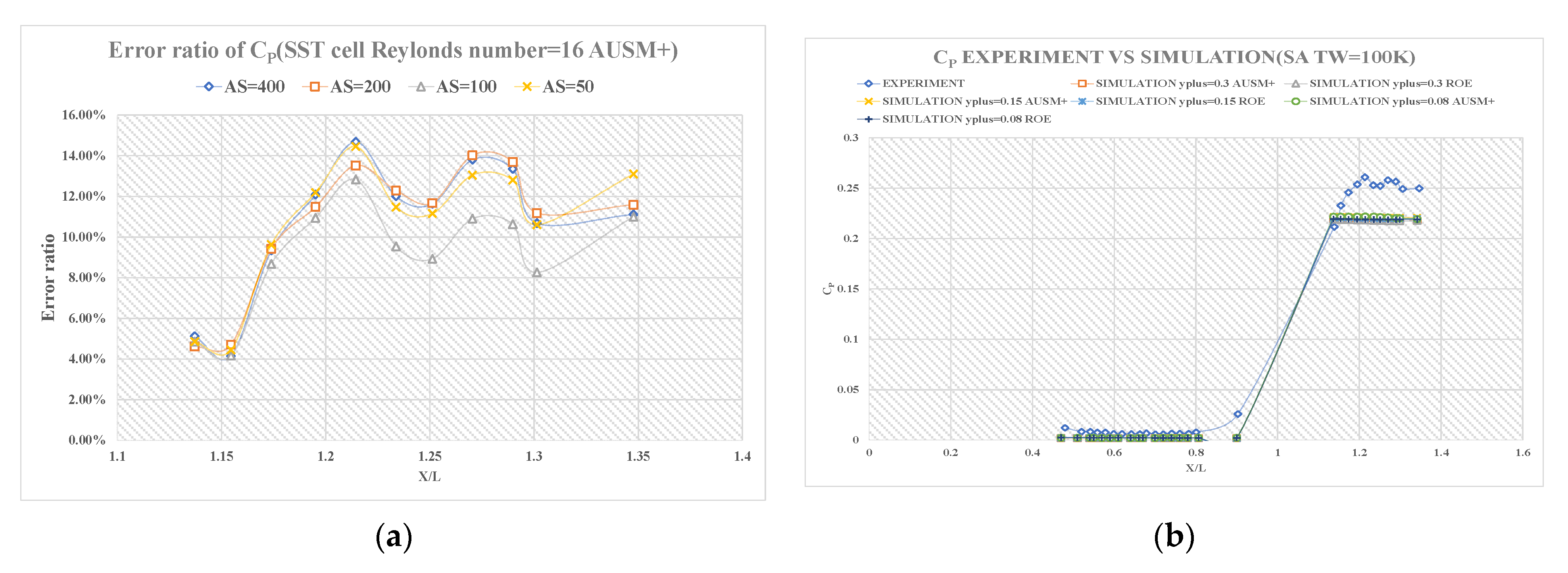
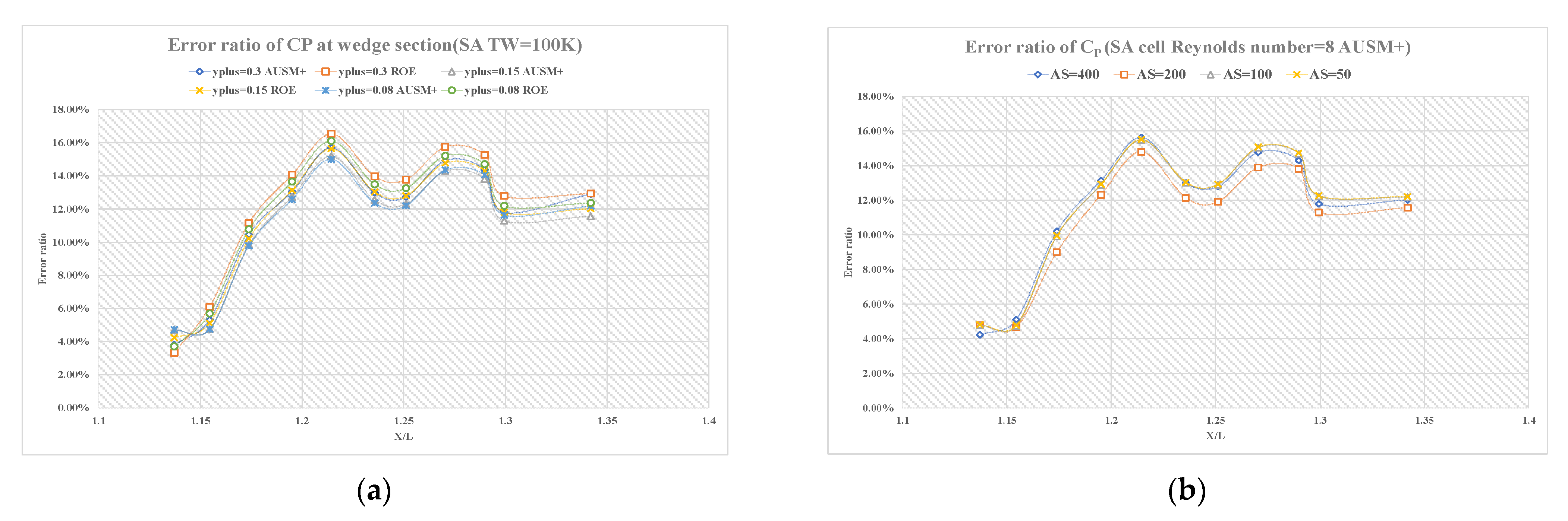
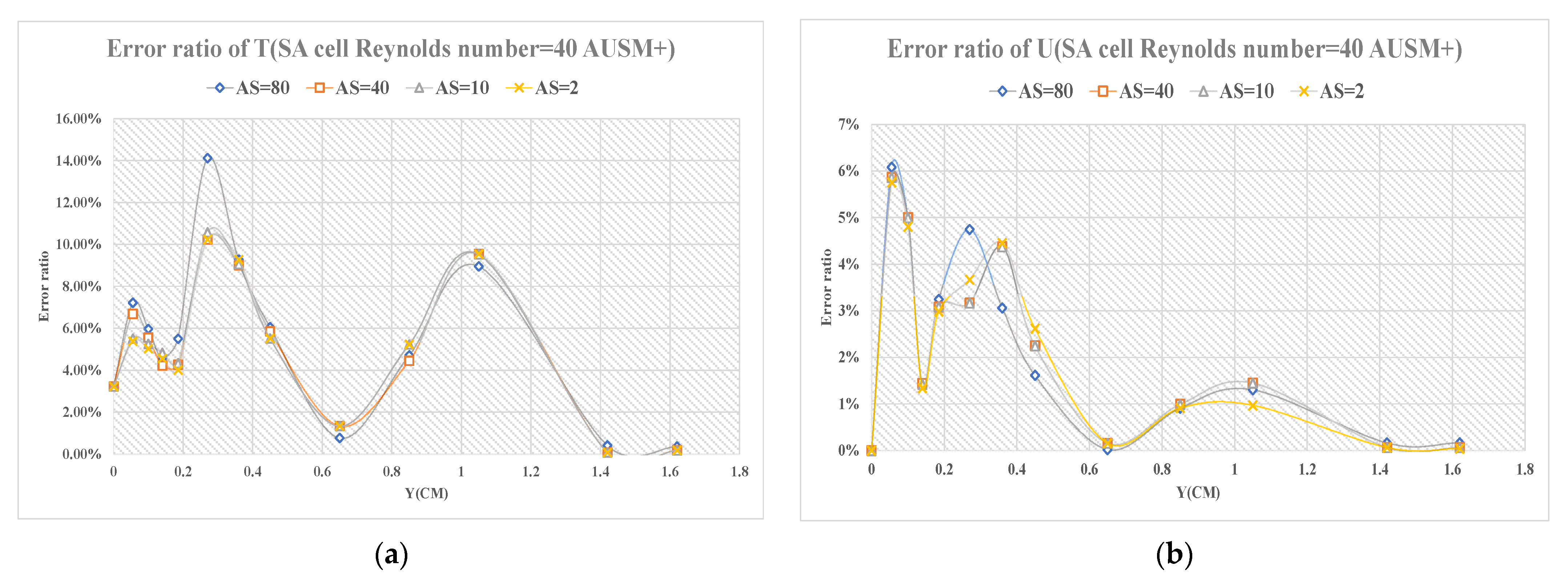
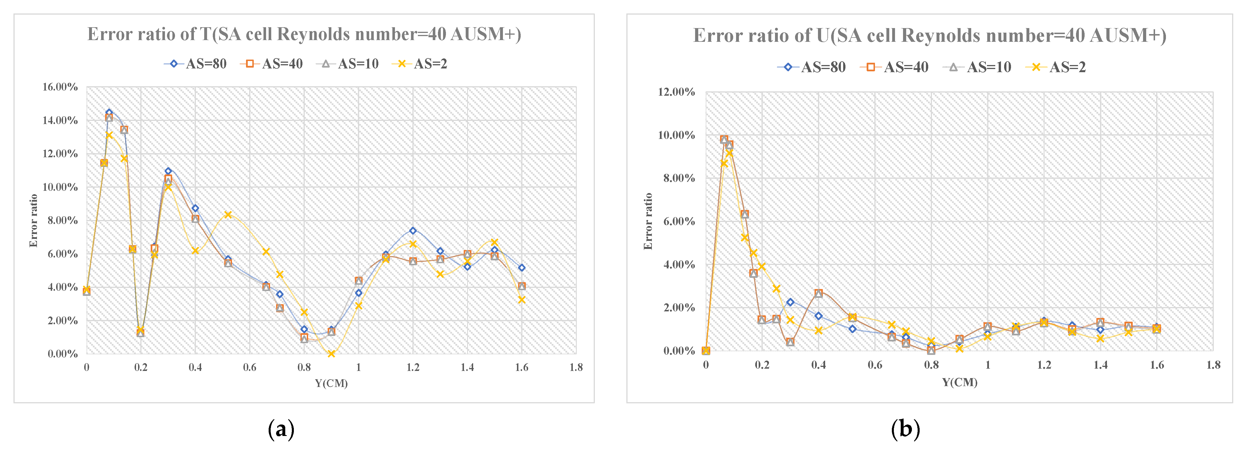
• For the wedge section in the scramjet-propelled vehicle heating prediction, the suggested value of cell Reynolds number and aspect ratio of wall cells near the shock are different from those for blunt bodies. At the high supersonic stage, the ideal cell Reynolds number should be no larger than 16. At the hypersonic stage, neither the ideal cell Reynolds number, nor the aspect ratio of the wall cells near the shock should be larger than 40.
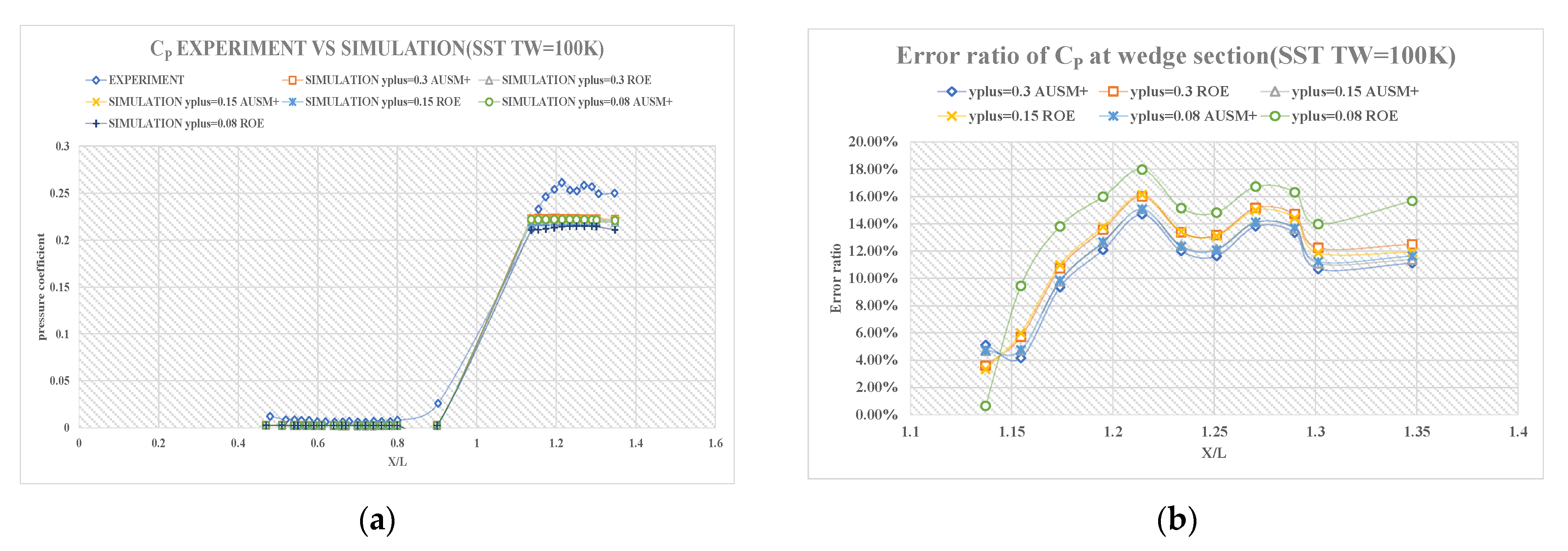
• For the wedge section in the scramjet-propelled vehicle heating prediction, with the same grid strategy, upwind scheme, solver, and so on, the AUSM+ flux type performs better than Roe’s FDS flux type. The Spalart-Allmaras turbulence model performs better at the transonic stage and the hypersonic stage, while the SST k-omega performs better at the supersonic stage and the high supersonic stage.
• Smaller cell Reynolds numbers are not necessarily better. On the one hand, this may cause the quality of the mesh to decrease. On the other hand, as described in Section 3.3 and Section 3.4, their improvement of calculation accuracy is limited; they even reduce the accuracy. The value of the aspect ratio is similar to the cell Reynolds number. It is necessary to confirm the appropriate values through CFD analysis based on numerical results and TVR plots.

References

1. Chen, F.; Liu, H.; Zhang, S. Time-adaptive loosely coupled analysis on fluid–thermal–structural behaviors of hypersonic wing structures under sustained aeroheating. Aerosp. Sci. Technol. 2018, 78, 620–636. [Google Scholar] [CrossRef]
2. Qu, F.; Kong, W.; Sun, D.; Bai, J. Shock-stable flux scheme for predicting aerodynamic heating load of hypersonic airliners. Sci. China Ser. G: Physics, Mech. Astron. 2019, 62, 984711. [Google Scholar] [CrossRef]
3. Tao, W.Q. Advances in Computational Heat Transfer, 1st ed.; Science Press: Beijing, China, 2002. (In Chinese) [Google Scholar]
4. Qu, F.; Sun, D.; Bai, J.; Zuo, G.; Yan, C. Numerical investigation of blunt body’s heating load reduction with combination of spike and opposing jet. Int. J. Heat Mass Transf. 2018, 127, 7–15. [Google Scholar] [CrossRef]
5. Qu, F.; Chen, J.; Sun, D.; Bai, J.; Yan, C. A new all-speed flux scheme for the Euler equations. Comput. Math. Appl. 2019, 77, 1216–1231. [Google Scholar] [CrossRef]
6. Cook, C.; Balachandar, S.; Chung, J.; Vu-Quoc, L. A generalized Characteristic-Based Split projection method for Navier-Stokes with real fluids. Int. J. Heat Mass Transf. 2018, 124, 1045–1058. [Google Scholar] [CrossRef]
7. Tsien, H.-S. Superaerodynamics, Mechanics of Rarefied Gases. J. Aeronaut. Sci. 1946, 13, 653–664. [Google Scholar] [CrossRef]
8. Lee, J.; Rho, O.H. Accuracy of AUSM+ Scheme in Hypersonic Blunt Body Flow Calculations, 8th ed.; AIAA International Space Planes and Hypersonic Systems and Technologies Conference: Norfolk, VA, USA, 1998. [Google Scholar]
9. Xiang, Z.; Chao, Y.; Wei, Y.; Haibo, H. Investigation of the grid-dependency in heat transfer simulation for hypersonic vehicle. Tactical Missile Technol. 2016, 3, 21–27. (In Chinese) [Google Scholar]
10. Qu, F.; Sun, D.; Zuo, G. A study of upwind schemes on the laminar hypersonic heating predictions for the reusable space vehicle. Acta Astronaut. 2018, 147, 412–420. [Google Scholar] [CrossRef]
11. Di Venuta, I.; Petracci, I.; Angelino, M.; Boghi, A.; Gori, F. Numerical simulation of mass transfer and fluid flow evolution of a rectangular free jet of air. Int. J. Heat Mass Transf. 2018, 117, 235–251. [Google Scholar] [CrossRef] [Green Version]
12. Kitamura, K.; Shima, E.; Nakamura, Y.; Roe, P.L. Evaluation of Euler Fluxes for Hypersonic Heating Computations. AIAA J. 2010, 48, 763–776. [Google Scholar] [CrossRef]
13. Qu, F.; Sun, D.; Yan, C. A new flux splitting scheme for the Euler equations II: E-AUSMPWAS for all speeds. Commun. Nonlinear Sci. Numer. Simul. 2018, 57, 58–79. [Google Scholar] [CrossRef]
14. Qu, F.; Chen, J.; Sun, D.; Bai, J.; Zuo, G. A grid strategy for predicting the space plane’s hypersonic aerodynamic heating loads. Aerosp. Sci. Technol. 2019, 86, 659–670. [Google Scholar] [CrossRef]
15. Smirnov, N.; Penyazkov, O.; Sevrouk, K.; Nikitin, V.; Stamov, L.; Tyurenkova, V. Detonation onset following shock wave focusing. Acta Astronaut. 2017, 135, 114–130. [Google Scholar] [CrossRef]
16. Li, J.Z.; Yan, C.; Ke, L.; Zhang, S.T. Research on scheme effect of computational fluid dynamics in aerothermal. J. Beijing Univ. Aeronaut. Astronaut. 2003, 11, 1022–1025. (In Chinese) [Google Scholar]
17. Yang, J.L.; Liu, M. Influence of limiters on numerical simulation of heating distributions for hypersonic bodies. J. Beijing Univ. Aeronaut. Astronaut. 2014, 40, 417–421. (In Chinese) [Google Scholar]
18. Zheng, X.; Liu, Z.-S.; Yang, Y.; Lei, J.-C.; Li, Z.-X. Research on Climb-cruise Global Trajectory Optimization for RBCC Hypersonic Vehicle. Missiles Space Veh. 2018, 47, 1–8. (In Chinese) [Google Scholar]
19. Speed of Sound. Available online: https://www.grc.nasa.gov/www/k-12/airplane/sound.html (accessed on 13 May 2021).
20. Spalart, P.; Allmaras, S. A one-equation turbulence model for aerodynamic flows. Rech. Aerosp. 1994, 1, 5–21. [Google Scholar]
21. Menter, F.R. Two-equation eddy-viscosity turbulence models for engineering applications. AIAA J. 1994, 32, 1598–1605. [Google Scholar] [CrossRef] [Green Version]
22. Jameson, A.; Schmidt, W.; Turkel, E. Numerical solution of the Euler equations by finite volume methods using Runge Kutta time stepping schemes. In Proceedings of the 14th Fluid and Plasma Dynamics Conference, Palo Alto, CA, USA, 23–25 June 1981; p. 1259. [Google Scholar]
23. Liepmann, H.W.; Bryson, A.E. Transonic Flow Past Wedge Sections. J. Aeronaut. Sci. 1950, 17, 745–755. [Google Scholar] [CrossRef]
24. Matin, R.K.; Ghassemi, H.; Arzideh, M.H. Numerical Study of the Effect of Geometrical Changes on the Airfoil Aerodynamic Performance. Int. J. Fluid Mech. Res. 2016, 43, 28–38. [Google Scholar] [CrossRef]
25. Chorin, A.J. Numerical solution of the Navier-Stokes equations. Math. Comput. 1968, 22, 745. [Google Scholar] [CrossRef]
26. Barth, T.; Jespersen, D. The design and application of upwind schemes on unstructured meshes. In Proceedings of the 27th Aerospace scIences Meeting, Reno, NV, USA, 9–12 January 1989; p. 366. [Google Scholar]
27. Stephen, E.; Dunagan, J.L.; John, B.; Miles, B. Interferometric Data for a Shock wave/Boundary-Layer Interaction. In NASA Technical Memorandum 88227; NASA Ames Research Center: Moffett Field, CA, USA, 1986. [Google Scholar]
28. Delery, J.; Coet, M.C. Experiments on Shock-Wave/Boundary-Layer Interactions Produced by Two-Dimensional Ramps and Three-Dimensional Obstacles. In Hypersonic Flows for Reentry Problems Désidéri; Glowinski, J.A., Périaux, R.J., Eds.; Springer: Berlin/Heidelberg, Germany, 1990. [Google Scholar]
29. Weiss, J.M.; Smith, W.A. Preconditioning applied to variable and constant density flows. AIAA J. 1995, 33, 2050–2057. [Google Scholar] [CrossRef]
30. Roe, P.L. Characteristic-Based Schemes for the Euler Equations. Annu. Rev. Fluid Mech. 1986, 18, 337–365. [Google Scholar] [CrossRef]
31. Chima, R.; Liou, M.-S. Comparison of the AUSM+ and H-CUSP Schemes for Turbomachinery Applications. In NASA Technical Memorandum 212457; NASA Glenn Research Center: Cleveland, OH, USA, 2003. [Google Scholar]
32. Kussoy, M.I.; Horstman, C.C. Documentation of Two-and Three-Dimensional Hypersonic Shock Wave/Turbulent Boundary Layer Interaction Flows. In NASA Technical Memorandum 101075; NASA Ames Research Center: Moffett Field, CA, USA, 1989. [Google Scholar]
33. Earl, T. Thermal Structures for Aerospace Applications; AIAA Press: Reston, VA, USA, 1996; p. 5. [Google Scholar]
34. Wu, D.F.; Shang, L.; Pu, Y.; Wang, H.T.; Gao, Z.T. Experimental research of thermal-insulation performance of lightweight thermal protection materials for hypersonic aircraft in oxidation environment up to 1700 °C. Spacecr. Environ. Eng. 2016, 33, 7–12. [Google Scholar]
35. Wu, D.F.; Lin, L.J.; Wu, W.J.; Sun, C.C. Experimental research on thermal/vibration test of lightweight insulation material for hypersonic vehicle under extreme-high-temperature environment up to 1500 °C. Acta Aeronaut. Astronaut. Sin. 2020, 41, 216–225. [Google Scholar]
Figure 1. (a) X51A; (b) The flight path of an RBCC scramjet-propelled vehicle. The initial conditions of flow at different phases are as follows: Climbing phase: (1) ejection phase, duration time is about 10 s. Flight altitude is about 11 km, Mach number is 0.8, pressure is 22,700 Pa, temperature is 216.77 K, air density is 0.3648 kg/m3 and dynamic viscosity is 1.422 × 10⁻⁵ Pa·s. (2) sub-combustion stamping phase, duration time is about 20 s. Flight altitude is about 16 km, Mach number is 3, pressure is 10,350 Pa, temperature is 216.65 K, air density is 0.1663 kg/m3 and dynamic viscosity is 1.422 × 10⁻⁵ Pa·s. (3) super-combustion stamping phase, duration time is about 4 s, flight altitude is about 26 km, Mach number is 6, pressure is 2188 Pa, temperature is 222.54 K, air density is 0.0339 kg/m3 and dynamic viscosity is 1.454 × 10⁻⁵ Pa·s. Cruising phase: the flight altitude is about 30 km, Mach number is 6.5, pressure is 1197 Pa, temperature is 226.51 K, air density is 0.0181 kg/m3 and dynamic viscosity is 1.475 × 10⁻⁵ Pa·s.
Applsci 11 09344 g001
Figure 2. The external flow field simulation model for the transonic stage.
Applsci 11 09344 g002
Figure 3. Yplus of 1 with 20 inflation layers.
Applsci 11 09344 g003
Figure 4. (a) computational domain; (b) close view of grids in and near the WALL region.
Applsci 11 09344 g004
Figure 5. Local Mach number versus x/c for different Mach numbers of freestream.
Applsci 11 09344 g005
Figure 6. The external flow field simulation model for the supersonic stage.
Applsci 11 09344 g006
Figure 7. (a) computational domain; (b) close view of grids in near shock wave region.
Applsci 11 09344 g007
Figure 8. (a) surface-pressure distributions from experiment and SST k-omega simulation; (b) surface-pressure distributions from experiment and Spalart-Allmaras simulation.
Applsci 11 09344 g008
Figure 9. (a) density profile at x = 0 from experiment and SST k-omega simulation; (b) density profile at x = 0 from experiment and Spalart-Allmaras simulation.
Applsci 11 09344 g009
Figure 10. The external flow field simulation model for the high supersonic stage.
Applsci 11 09344 g010
Figure 11. (a) computational domain; (b) close view of grids in near shock wave region.
Applsci 11 09344 g011
Figure 12. (a) wall pressure coefficient distribution diagram adopting SST K-omega at TW = 100 K; (b) error ratio of wall pressure coefficient distribution diagram at the wedge section adopting SST K-omega at TW = 100 K.
Applsci 11 09344 g012
Figure 13. (a) error ratio of wall pressure coefficient distribution diagram at the wedge section adopting four different aspect ratios; (b) wall pressure coefficient distribution diagram adopting Spalart-Allmaras at TW = 100 K.
Applsci 11 09344 g013
Figure 14. (a) error ratio of wall pressure coefficient distribution diagram at the wedge section adopting Spalart-Allmaras at TW = 100 K; (b) error ratio of wall pressure coefficient distribution diagram at the wedge section adopting four different aspect ratios.
Applsci 11 09344 g014
Figure 15. (a) wall pressure coefficient distribution diagram adopting SST K-omega at TW = 290 K; (b) error ratio of wall pressure coefficient distribution diagram at the wedge section adopting SST K-omega at TW = 290 K.
Applsci 11 09344 g015
Figure 16. (a) error ratio of wall pressure coefficient distribution diagram at the wedge section adopting four different aspect ratios; (b) wall pressure coefficient distribution diagram adopting Spalart-Allmaras at TW = 290 K.
Applsci 11 09344 g016
Figure 17. (a) error ratio of wall pressure coefficient distribution diagram at the wedge section adopting Spalart-Allmaras at TW = 290 K; (b) error ratio of wall pressure coefficient distribution diagram at the wedge section adopting four different aspect ratios.
Applsci 11 09344 g017
Figure 18. The external flow field simulation model for the high supersonic stage.
Applsci 11 09344 g018
Figure 19. (a) computational domain; (b) close view of grids in near shock wave region.
Applsci 11 09344 g019
Figure 20. (a) ratio distribution diagrams between T and TINF at S = 0.055 m; (b) ratio distribution diagrams between U and UINF at S = 0.055 m.
Applsci 11 09344 g020
Figure 21. (a) ratio distribution diagrams between T and TINF at S = 0.105 m; (b) ratio distribution diagrams between U and UINF at S = 0.105 m.
Applsci 11 09344 g021
Figure 22. (a) ratio distribution diagrams between T and TINF at S = 0.155 m; (b) ratio distribution diagrams between U and UINF at S = 0.155 m.
Applsci 11 09344 g022
Figure 23. (a) error ratio distribution diagrams of T at S = 0.005 m; (b) error ratio distribution diagrams of U at S = 0.005 m.
Applsci 11 09344 g023
Figure 24. (a) error ratio distribution diagrams of T at S = 0.105 m; (b) error ratio distribution diagrams of U at S = 0.105 m.
Applsci 11 09344 g024
Figure 25. (a) error ratio distribution diagrams of T at S = 0.155 m; (b) error ratio distribution diagrams of U at S = 0.155 m.
Applsci 11 09344 g025
Figure 26. The simulation model for aerothermal prediction of RBCC scramjet-propelled vehicle.
Applsci 11 09344 g026
Figure 27. The aerodynamic heat prediction for RBCC scramjet-propelled vehicle in the flight path.
Applsci 11 09344 g027