Tempcore™ is the trademark for the heat treatment route that was developed in the 1970s by CRM Group and has since been widely used for the manufacturing of reinforcing steel bars (rebars) [
1,
2]. It is a quench and self-tempering thermo-mechanical process wherein the hot rolled rebars come out of the last hot-rolling mill at a temperature above
at which the rebars are still in their austenitic state and then are rapidly quenched with water sprayed onto their surface at high volumetric flow rate. The outer layer of the rebar transforms from austenite to martensite up to a certain depth. The time of quenching and the volume of water sprayed are controlled to achieve the desired thickness of the outer martensitic layer for a given diameter of the rebar, and below this depth the core is still austenitic. The rebar is then left to cool in the cooling bed, where the core transforms to a ferrite and pearlite mixture while the heat dissipating from the core tempers the martensitic layer, hence the name Tempcore. The process is schematically presented in
Figure 1. This composite nature of the rebar with an outer hard layer and a ductile inner core is achieved with a relatively simple heat treatment process that produces high-strength rebars that are bendable and weldable without the need for micro-alloying with V or Nb [
1,
2,
3].
The Tempcore™ process often has been investigated from the point of view of strength and corrosion resistance [
4,
5,
6,
7], fatigue behavior during service [
8], behavior at high temperatures [
9], and effects of their geometry [
10]. Very few studies could be found in the literature that investigate the residual stresses that are generated during the manufacturing process itself. The research project from which this report is extracted aims at understanding the links between fatigue performance and residual stresses in the rebars, with the goal to enhance their fatigue life. It is well established that macroscopic compressive surface residual stresses enhance the fatigue performance of the material by closing fatigue cracks that usually initiate near the surface. On the other hand, tensile residual stresses lead to premature failure of parts by aiding crack growth and could also lead to stress corrosion cracking [
11,
12]. In service, the residual stresses are superimposed with the external load stresses and can be either beneficial or sometimes catastrophically detrimental by lowering the stresses at which cracks initiate to dangerously low levels [
13].
1.1. Origin of Residual Stresses during Quenching
The residual stresses in the finished product are a consequence of the asynchronous thermal shrinkage and phase transformation of the core and the surface regions. During quenching all materials are exerted to shrinkage stresses since the surface always cools faster than the core. Additionally, if phase transformations occur during quenching, transformation stresses ensue as well and superimpose on the aforementioned shrinkage stresses. In order to understand the origin of the residual stresses during quenching and thereby the factors that affect it, a closer look at the generation of these two types of stress is necessary. The top part of
Figure 2 shows the cooling curves of the surface and the core of a cylinder during quenching
together with the yield stress,
of these regions, which depends on the temperature and hence on process time and is assumed to be the same for compression and tension. For simplicity, only the longitudinal stress component is shown, although criteria for plastic flow also consider the tangential and radial components [
14,
15,
16].
Concentrating only on the shrinkage stresses on the left side, the surface cools faster than the core at the initial stage of the quench. This results in longitudinal tensile stresses at the surface, whereas the core experiences longitudinal compressive stresses. As long as there is no plastic deformation, these stresses will be balanced at the end of the process with no residual stresses, as can be seen in the middle part of
Figure 2a. Usually, however, these shrinkage stresses exceed the yield stress of the material shown as a gray shaded area in the figure. This is promoted by the low yield stress at high temperatures where the temperature gradients are very high [
10,
15]. Therefore, the material flows plastically leaving residual stresses at the end as shown in the bottom part of
Figure 2a. Upon further cooling the core temperature falls rapidly while the surface gradually reaches the temperature of the cooling medium, thus reducing the magnitude of the shrinkage stresses and eventually reversing their signs. The plastic stretching of the surface causes compression at the surface and vice versa in the core. Once the temperature balance is established, the cylinder is left with compressive stresses at the surface and tensile stresses in the core due to the shrinkage stresses.
If the phase transformation in the material is to be considered, the same line of reasoning could be laid out for pure transformation stresses ignoring the thermal shrinkage stresses and transformation plasticity. The top part of
Figure 2b shows the cooling curves of the surface and the core of the cylinder, the martensite start and finish temperatures,
and
, and the temperature-dependent yield stress of the material. Upon reaching
it is assumed that the whole material transforms into martensite, which occurs at times
at the surface and
in the core. The volume expansion associated with the austenite to martensite transformation, which is ca. 3.4% for 0.19 % C steel [
17], leads to compressive stresses arising near the surface compensated by tensile stresses in the core as shown in the middle part of
Figure 2b. Once the core reaches
and starts to transform and expand, the stresses are reduced in both regions. Due to the transformation into much harder martensite, the yield stress curves undergo a much larger increase in magnitude than in the case of mere thermal shrinkage as shown in
Figure 2a, left. The plastic flow occurring due to the transformation stresses exceeding the yield point (shown in gray) results in volume incompatibilities between the core and the surface at the end of the cycle. This leads to residual stresses, which are shown at the bottom of
Figure 2b by arrows, which are reversed in sign compared to the left image.
Combining these two types of stress by simple superposition is not accurate, since the material has deformed plastically. The fundamental concept from this discussion is, however, helpful in understanding the factors involved in solving such problems and the material parameters required for modeling such a quenching process successfully. It is clear that the yield stress of the material at high temperatures determines plastic flow and has to be quantified. The relative position of the time in which the transformation initiates and ends at the surface and in the core significantly influences the magnitude as well as the sign of the final residual stresses [
14].
To the best of the authors’ knowledge these parameters are not available in literature for the B500B alloy, which constitutes a large fraction of commercially available rebars and, hence, have to be determined experimentally. Some attempts have been made to predict the strength and transformation temperatures with models and theoretical calculations [
5]. The thermal history or the cooling curve across the cross section of the bar during quenching and tempering is, however, impractical and prohibitively expensive to obtain directly from the manufacturing facility, if for this purpose the production of large tonnages has to be stopped. Therefore, several studies have been conducted to predict the transient temperature profile across the cross-section of the rebar with computational fluid dynamics simulations of the coolant coupled to the heat transfer problem in the rebar [
5,
18,
19].
In summary, the following facts are important to consider. The plastic deformation determines the magnitude of the residual stresses. The temperature difference between the surface and the core is dependent on the following factors: the starting temperature of the quenching process, the diameter, the heat transfer coefficient, and the thermal properties of the material. The residual stresses are larger in magnitude if the yield strength at high temperature is very low, due to larger plastic deformation. Finally, the residual stresses greatly depend on the relative initiation time of the transformation in the surface and core regions.
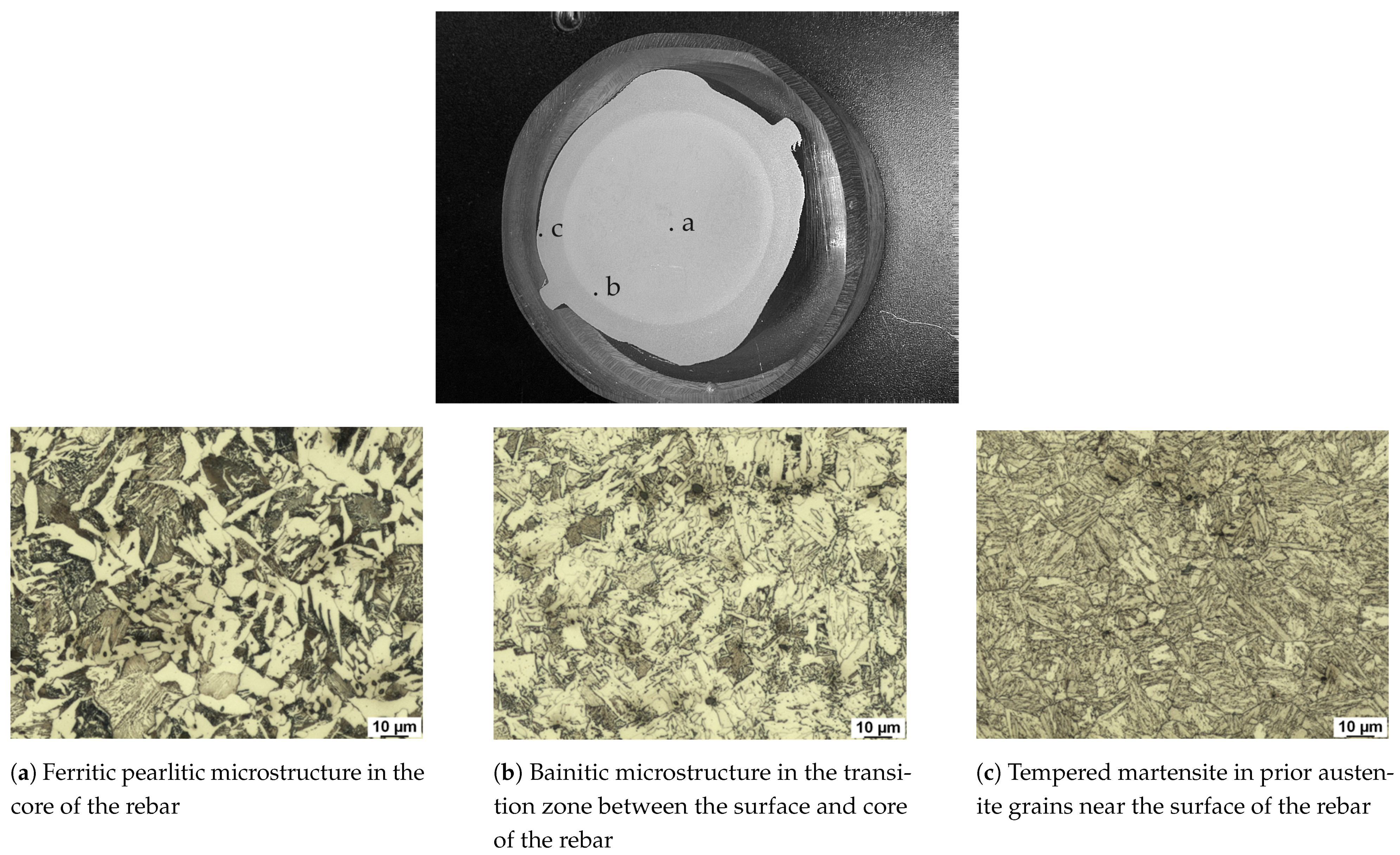
The phenomena that were neglected in the above discussion for simplicity need to be considered for solving real problems. The material as a whole will not transform into martensite, but rather a mixture of all the phases including ferrite, pearlite, bainite, and martensite is present in the rebar as will be seen in
Section 3.1. Only longitudinal stresses were considered, but the criteria for plastic flow usually consider all the components of stress [
16]. Furthermore, transformation plasticity effects that were neglected may have a significant influence on the residual stress distribution and should be examined [
20]. In addition to the material parameters, the geometry of the ribs on the rebar and its surface finish also significantly influence the fatigue behavior [
8]. Experimental determination of residual stresses, e.g., using X-ray diffraction, will reach their limitations for such complex surface geometry. Furthermore, the resolution is not high enough to measure the residual stresses at the foot of the ribs, which usually act as the origin of cracks in these bars. Hence, it is only through simulating the quenching process with the correct material parameters, material constitutive model, and rebar geometry that a better understanding of the process can be gained.
1.2. Constitutive Modeling for Numerical Investigations of the Tempcore™ Process
Since it is not feasible to inspect the transient stresses shown in
Figure 2 by in-process measurements, numerical simulations play an important role in understanding the generation of residual stresses during the heat treatment and thereby potentially attain further optimization of the process parameters. Given the requirement to resolve the macro-geometry of the considered component within the spatial discretization, constitutive modeling for heat treatment simulations is often based on component-scale continuum formulations where the microstructure is accounted for only be means of volume proportions of the existing phases [
5,
6,
19,
20]. In the simplest scenario, this approach typically involves solving the following initial boundary value problems (IBVPs):
The transient non-homogeneous isotropic heat equation governing heat conduction in the spatial domain
spanned by the solid and the temporal domain
with prescribed surface convection on
and a known initial temperature field
[
21]:
Here, , , and denote the density, specific heat capacity, and thermal conductivity of the compound, respectively, the coolant temperature, h the heat transfer coefficient, and the internal heat generation, e.g., due to latent heat associated with phase transformations or plastic dissipation.
The mechanical compatibility and (quasi-)static equilibrium equations [
21] where geometric linearity and negligence of body forces are typically suitable assumptions for heat treatment simulations [
20]:
In this system,
denotes the Cauchy stress tensor,
the linear strain tensor, and
the displacement field. Equations (
4) and (
5) are usually complemented with displacement- or traction-free boundary conditions on a partition
of the solid’s boundary (the outward normal of which is denoted as
) as well as stress- and displacement-free initial conditions:
To complete the description of the mechanical IBVP, a constitutive model that particularizes Equation (
5) must be specified, where the assumption of isotropic thermo-elasto-plastic behavior according to the classical flow theory of plasticity is almost universal in literature [
20]. This amounts to computing the stresses
from the elastic strains
as
where
is the eigenstrain due to thermal expansion (and potentially phase transformations) and
is the plastic strain computed by integration of the (associated) flow rule
subject to the constraints
,
(von Mises criterion) and
[
16]. In these equations,
and
denote the identity tensors of rank 2 and 4, respectively,
the stress deviator,
the plastic multiplier,
the yield strength, and
E and
Young’s modulus and the Poisson’s ratio, respectively.
In order to apply the above IBVPs to the numerical simulation of heat treatment of a solid compound of more than one phase, the material parameters encountered in above equations are most commonly computed via a linear volume-fraction averaged mixture rule from the respective parameters of the individual phases [
20]. For example, the yield strength
of a mixture of
P phases, each constituting a volume fraction
,
, of the microstructure at the considered point
of the continuum, may be assumed to adhere to
where
denotes the yield strength of phase
i. Furthermore, evolution equations describing the phase transformation kinetics in terms of the volume fractions
of each phase are required to evaluate such mixture rules.
It is apparent from the above presentation that any numerical computation of process-induced residual stresses based on a thermo-mechanical constitutive model of comparable complexity as above relies on the accurate identification of at least the following parameters for each phase encountered during the process: density, heat capacity, and conductivity for the heat transfer problem and Young’s modulus, Poisson’s ratio, and the yield strength for the mechanical problem. The aim of this paper is therefore to enable numerical heat-treatment simulations for rebars by experimental determination of the mechanical parameters for the alloy B500B.

 ,
, 


