Abstract
Assembly path planning of complex products in virtual assembly is a necessary and complicated step, which will become long and inefficient if the assembly path of each part is completely planned in the assembly space. The coincidence or partial coincidence of the assembly paths of some parts provides an opportunity to solve this problem. A path planning algorithm based on prior path reuse (PPR algorithm) is proposed in this paper, which realizes rapid planning of an assembly path by reusing the planned paths. The core of the PPR algorithm is a dual-tree fusion strategy for path reuse, which is implemented by improving the rapidly exploring random tree star (RRT *) algorithm. The dual-tree fusion strategy is used to find the nearest prior node, the prior connection node, the nearest exploring node, and the exploring connection node and to connect the exploring tree to the prior tree after the exploring tree is extended to the prior space. Then, the optimal path selection strategy is used to calculate the costs of all planned paths and select the one with the minimum cost as the optimal path. The PPR algorithm is compared with the RRT * algorithm in path planning for one start node and multiple start nodes. The results show that the total time and the number of sampling points for assembly path planning of batch parts using the PPR algorithm are far less than those using the RRT * algorithm.
1. Introduction
Digital assembly is one of the key technologies in the design and manufacturing of complex products [1,2,3,4]. Some technologies, such as virtual reality (VR), augmented reality (AR), digital prototyping (DP), and digital twin (DT) assembly, are used to realize the design, verification, and optimization of an assembly in a virtual environment by virtual reality fusion and interactive control and to improve the assembly quality and efficiency of complex products [5,6,7,8,9,10,11,12,13].
Assembly planning (AP) is one of the most important bases and premises of the assembly process and has some main subproblems: assembly sequence planning (ASP), assembly motion planning (AMP), assembly resource planning (ARP), assembly path planning (APP), etc. These problems have proven to be either non-deterministic polynomial hard (NP-hard) or non-deterministic polynomial complete (NP-complete), and many studies have been conducted to solve them efficiently [14,15,16,17,18,19].
The methods proposed for ASP include a scatter search optimization algorithm [15], ant colony optimization algorithm [20], case-based reasoning algorithm [21], improved particle swarm optimization method [22], etc. The methods proposed for AMP include the rapidly exploring random trees method [23], rapidly exploring deterministic tree method [24], curve-matching method [25], etc. The methods proposed for ARP include a digital twin method [26], geometric reasoning method [27], modularity and reconfiguration method [28], intelligent collaboration method [29], etc. The methods proposed for APP include a particle swarm optimization approach [30], potential field method [31], centroidal Voronoi tessellation algorithm [32], exemplary K-nearest neighbor interpolation approach [33], etc.
The APP of a complex product takes much time due to the large number of parts; thus, the optimization of APP will improve assembly efficiency [33]. In addition to the above-mentioned APP methods, there have also been some studies on robot path planning [34,35,36], vehicle path planning [37,38,39], UAV path planning [40,41,42], etc. For most of the APP methods mentioned above, it takes a large amount of repeated computation and leads to low planning efficiency and high costs if generating the assembly path through all parts.
In these studies, rapidly exploring random tree (RRT) and probabilistic roadmap planners (PRM) are two typical random sampling algorithms in path planning. The PRM algorithm constructs the road map in the space by random sampling and seeks a feasible solution based on graph searching [43,44]. However, the PRM algorithm consumes high costs and is not suitable for a dynamic environment [45].
The RRT algorithm is an effective method which explores free space by expanding a tree structure with the leaf nodes generated randomly and uniformly. When a leaf node reaches the target area, a collision-free path is obtained by backtracking from the leaf node to the parent node in sequence [23,46].
Although the RRT algorithm is an efficient algorithm in path planning, the randomness of the sampling points makes it difficult to obtain the optimal path even if the number of sampling points is sufficient. Therefore, some algorithms have been proposed to improve the RRT algorithm in terms of random point generation, nearest point selection, interference detection, and node connection [47,48,49]. One of them is the rapidly exploring random tree star (RRT *) algorithm, which makes the path cost lower by improving the nearest point selection strategy [50,51].
However, the RRT * algorithm cannot obtain a low-cost assembly path in a short time, or even a valid assembly path when the number of sampling points is small.
In fact, the assembly paths of many parts of a complex product are coincident or partially coincident, resulting in a large number of repeated calculations in path planning. Therefore, a path planning algorithm based on prior path reuse (PPR algorithm) is proposed as follows: (1) the assembly path is segmented and the configuration space is constructed, and (2) the prior path is reused, and the dual-tree fusion strategy and the optimal path selection strategy are performed. The proposed method in this paper performs well with a small sampling size which reduces repeated calculations by reusing planned assembly paths and improves the efficiency of new path planning.
2. Establishment of Prior Path Space
2.1. Segmentation of the Assembly Path
The assembly paths of different parts in a complex product are varied; thus, it is difficult to reuse an assembly path completely. A feasible method is to segment the assembly path and then reuse it [52]. Based on a method of segmenting the assembly path into two phases, the assembly path of a part is divided into three phases in turn by four key positions of the part from the shelf to assembly in this paper, as shown in Figure 1. The four positions are the initial point, the start point, the end point, and the target point, and the three phases are the handling phase, the logistics phase, and the assembly phase.

Figure 1.
Segmentation of an assembly path.
In the handling phase, the part is transferred from the initial point (the position where the part is stored on the shelf) to the start point (the position where the part is waiting to be transported near the shelf). In the logistics phase, the part is transported from the start point to the end point (the position where the part is waiting to be assembled near the assembly), bypassing various obstacles. In the assembly phase, the part is transferred from the end point to the target point (the final position where the part is assembled) after position-posture transformation.
Since the initial point, the start point, and the target point of each part are typically different, it is difficult to plan the handling phase and the assembly phase of a new assembly path by reusing the corresponding phases of other planned paths.
However, in the logistics phase, all the parts can be moved to the same position before assembly, which means that their end points are the same. Two assembly paths with the same end point may coincide within a certain range even if their start points are different, which makes the reuse of the logistics phase of planned paths possible. Therefore, the path reuse in this paper focuses on the logistics phase.
2.2. Transformation from Assembly Space to Configuration Space
A large number of parts, assembly tools, workbenches, and various auxiliary equipment in the assembly space are obstacles that need to be bypassed in APP, which leads to a high complexity of collision detection and a low efficiency of path planning.
Therefore, the configuration space method is usually used to model the assembly space [53], which maps the assembly space into a two-dimensional configuration space containing the obstacle space and the free space. The assembly path can be solved by using a two-dimensional path planning algorithm in the configuration space, which is helpful to reduce the difficulty and improve the efficiency of path planning.
In this paper, in addition to the obstacle space and the free space, the configuration space also contains the prior path space constructed by the planned assembly paths. The paths in the prior space constitute a prior path set, which is described by a tree structure, as shown in Figure 2. Each prior path is composed of the nodes in sequence from the start node (the leaf node) xstart_i (i = 1, …, m) to the end node (the root node) xend with some nodes pij (i = 1, …, m; j = 1, …, n) between them. Therefore, the path planning for the logistics phase in the assembly space is converted into a non-interference path search from the start node to the end node in the configuration space.
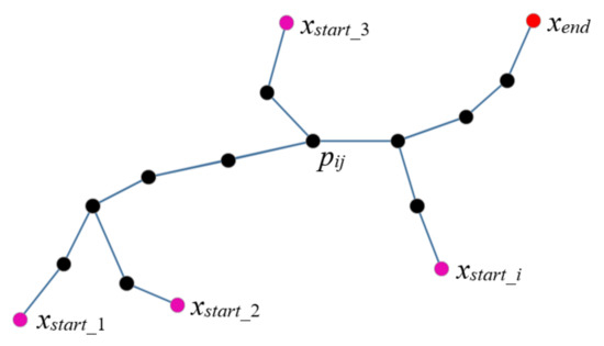
Figure 2.
Tree structure of a prior path set.
A path planning algorithm based on RRT expands the path by generating random points in the configuration space and detects collision interference by connecting the points with lines. If a prior path is represented only by some nodes of the tree, the probability that the sampling points happen to be generated on these nodes is extremely small. Therefore, a prior path tree is inflated into a prior path space [54] which is helpful for improving the reusability of a prior path.
There are two steps to inflate a path tree into a path space. First, each node of the tree is expanded into a circle, where the radius of the circle is positively related to the number of parts that appear at the node and the size of their bounding volume. In the process of moving parts from the start node to the end note, the size of parts consumes some space along the assembly path which cannot be ignored. Therefore, this virtual space is applied to simulate the real space which is consumed by the size of each part, and the radius of each circle can be changed to adjust the envelope of the path space in a real application. Second, the outer common tangents of each two adjacent circles are connected in sequence to construct the prior path space. The prior path tree shown in Figure 2 is inflated into the prior path space shown in Figure 3.
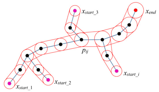
Figure 3.
Prior path space.
3. The Path Planning Algorithm Based on PPR
3.1. Prior Path Reuse in the PPR Algorithm
The PPR algorithm proposed in this paper improves the RRT * algorithm by developing some prior path reuse strategies to rapidly generate an asymptotically optimal assembly path by reusing the prior paths after the path exploring tree is expanded to the prior path space.
The main steps of assembly path reuse in the PPR algorithm are as follows:
Step 1. A new node xnew is generated with a given step S on the line connecting the random node xrand and the nearest node xnear, as shown in Figure 4.
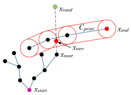
Figure 4.
Generation of xnew.
Step 2. The position of xnew in the configuration space is detected to determine the next step: (1) in the obstacle space Cobs, return to Step 1; (2) in the free space Cfree, optimize the exploring tree with the RRT * algorithm; and (3) in the prior space Cprior, proceed to Step 3 for path reuse planning.
Step 3. Two connection nodes pconnect and xconnect are identified for path reuse by using a dual-tree fusion strategy on the prior path tree Tprior and the exploring tree Texploring, respectively, as shown in Figure 5.
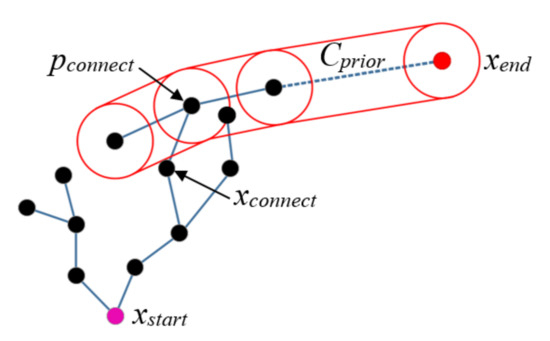
Figure 5.
Connection nodes.
Step 4. The new branch connecting xconnect and pconnect is added to Texploring, and a path Γi obtained by backtracking is added to the prior path set ψ, as shown in Figure 6.
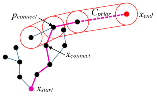
Figure 6.
Path backtracking.
Step 5. The minimum cost path Γmin is selected as the final path from ψ of all prior paths obtained after sampling N times. The cost of a path Γ is defined by the path length cost as , where denotes the Euclidean distance.
The above-mentioned steps illustrate the prior path reuse method in path planning from the start node xstart to the end node xend. After the exploring tree is expanded to the prior space, the node pair (xconnect, pconnect) connecting the exploring tree and the prior path tree is determined by the dual-tree fusion strategy, and then a path expressed as xstart-xconnect-pconnect-xend is obtained by backtracking from the end node xend to the start point xstart.
The pseudo-code of the PPR algorithm (Algorithm 1) is as follows:
| Algorithm 1. PPR algorithm |
| Input: Cplan, Cobstacle, Cprior, xstart, xend, S, N, Tprior, Texploring Result: A path Γ with the minimum cost from xstart to xend Texploring.init(); //Initialize the exploring tree Texploring Ψ.init(); //Initialize the prior path set Ψ for n = 1 to N do //Sample N times { xrand←Sample(Cplan); //Generate a random node xrand in the configuration space Cplan xnear←Near(xrand, Texploring); //Discover the nearest node xnear near xrand on Texploring xnew←Steer(xrand, xnear, S); //Generate a new node xnew between xrand and xnear with step S if CollisionFree(Cobstacle, xnew) then //Determine whether xnew is in the obstacle space Cobstacle { Xnear←Near (xnew, Texploring); //Create a set Xnear with the nodes on Texploring near xnew xmin←SelectParentNode(Xnear, xnear, xnew); //Select the minimum cost parent node of xnew Texploring.AddEdge(Edge(xmin, xnew)); //Add the new branch Edge(xmin, xnew) to Texploring Texploring.Rewire(); //Rewire the local part of the exploring tree near xnew for lower cost if InPriorSpace(Cprior, xnew) then //Determine whether xnew is in the prior space Cprior { xconnect, pconnect←ConnectNode(Texploring, Tprior, xnew); //Obtain the connection nodes pconnect, xconnect Texploring.AddEdge(xconnect, pconnect); //Add the new branch Edge(xconnect, pconnect) to Texploring Γi←PathBacktrack(Texploring, Tprior, xconnect, pconnect); //Obtain a path Γi by path backtracking Ψ.AddPath(Γi); //Add Γi to Ψ } } } Γmin←MinCostPath(Ψ); //Obtain the minimum cost path Γmin return Γmin; //Retrieve Γmin as the final path Γ |
The PPR method greatly reduces the number of samplings by reusing the prior path, which is helpful to improve the efficiency of APP.
3.2. Dual-Tree Fusion Strategy
The key aspect of the dual-tree fusion strategy is the determination of the node pair (xconnect, pconnect) connecting the path exploring tree Texploring and the prior path tree Tprior after the exploring tree is expanded into the prior space.
The main steps of the dual-tree fusion strategy are as follows:
Step 1. The prior nodes on the prior path in the circle with xnew as the centre and S as the radius are selected to create a nearest prior node set Pnear, as shown in Figure 7, where Pnear = {p2, p3}.
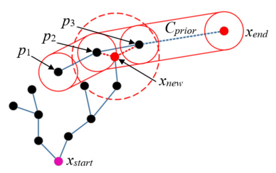
Figure 7.
Discovery of the nearest prior nodes.
Step 2. If the costs of nodes in Pnear are different, the node with minimum cost is selected as the connection node pconnect on the prior path; otherwise, the nearest node is selected. In Figure 7, p2 is selected as pconnect, as shown in Figure 8.
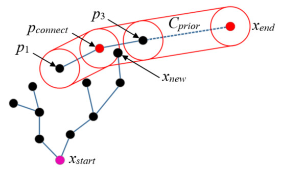
Figure 8.
Selection of the prior connection node.
Step 3. After the prior connection node pconnect is obtained, the exploring nodes on the exploring tree in the circle with pconnect as the center and S as the radius are selected to create a nearest exploring node set Xnear, as shown in Figure 9, where Xnear = {xnew, x1, x2}.
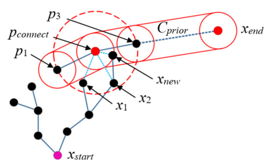
Figure 9.
Discovery of the nearest exploring nodes.
Step 4. If the costs of nodes in Xnear are different, the node with minimum cost is selected as the connection node xconnect on the exploring tree; otherwise, the nearest node is selected. In Figure 9, x1 is selected as xconnect, as shown in Figure 10.
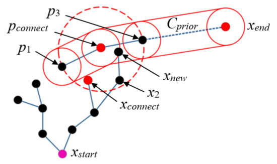
Figure 10.
Selection of the nearest exploring node.
3.3. The Optimal Path Selection Strategy
The path obtained according to the dual-tree fusion strategy is divided into the following two segments by the connection point pair (xconnect, pconnect): the prior path segment Γprior from the end node xend backtracking to the connection node pconnect on the prior path tree Tprior and the exploring path segment Γexploring from the connection node xconnect backtracking to the start node xstart on the exploring path tree Texploring, as shown in Figure 11.
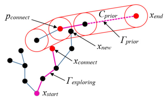
Figure 11.
Γprior and Γexploring.
As the number of sampling points increases, the cost of Γexploring is made asymptotically optimal by rewiring the exploring tree, and the shortest Γexploring can be obtained if the number of sampling points is sufficient, as shown in Figure 12.
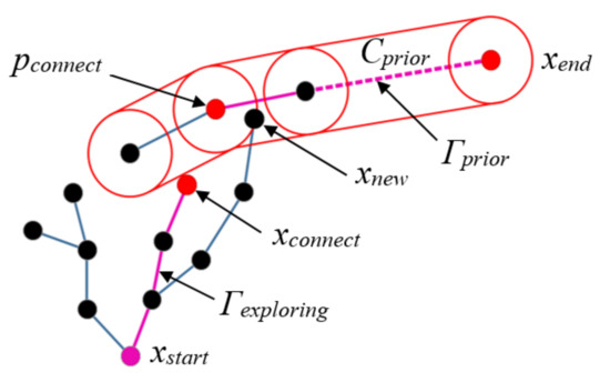
Figure 12.
The shortest Γexploring.
Since xnew is randomly generated in the prior space, the connection node pair (xconnect, pconnect) obtained by using the dual-tree fusion strategy may be different, such as (x1, p1), (x2, p2), and (xi, pi) shown in Figure 13; thus, the paths obtained according to these pairs are also different, indicated by Γ1, Γ2, and Γi, respectively, as shown in Figure 14.
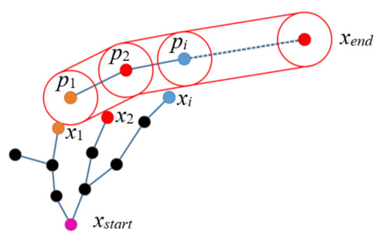
Figure 13.
Different connection node pairs.
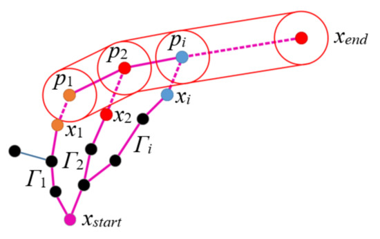
Figure 14.
Different paths.
Therefore, a planned path Γi based on reuse is expressed as Γi = Γprior_i + Γconnect_i + Γexploring_i, where Γprior_i is the prior path segment from pi to xend, Γconnect_i is the path segment from xi to pi, and Γexploring_i is the exploring path segment from xi to xstart, i = 1, …, m.
According to the composition of the path Γi, the cost of the path Γi is the sum of the costs of Γprior_i, Γconnect_i and Γexploring_i. Since Γconnect_i includes only two connection points and is determined by the minimum cost strategy, the cost of Γconnect_i is negligible due to its small impact on the total cost. Therefore, the cost of Γi is simplified to the sum of the costs of Γprior_i and Γexploring_i.
Considering that different parts have different dependences on paths Γprior and Γexploring, the weight coefficients ξprior and ξexploring are assigned to Γprior and Γexploring, respectively, and ξprior + ξexploring = 1. With an increase in ξprior, the optimal path asymptotically approaches the shortest prior path segment. With an increase in ξexploring, the optimal path asymptotically approaches the shortest exploring path segment.
4. Examples and Comparison
In this section, two case studies of assembly path planning are given to validate and demonstrate the application of the PPR algorithm, and the comparisons of results are illustrated as shown in Figure 15 and Figure 16. The start node, end node, and prior path of each case study are marked in the figures.
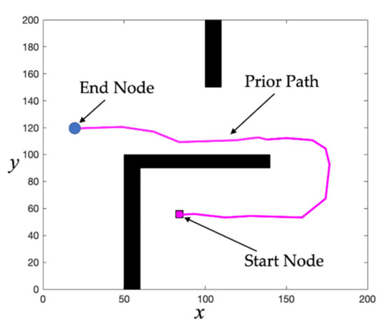
Figure 15.
Case Study 1.
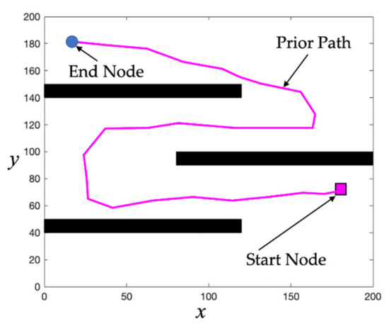
Figure 16.
Case Study 2.
4.1. Comparison of Results of PPR Algorithm with Different Numbers of Sampling Points
The PPR algorithm is used to plan the assembly path from xstart to xend with different maximum numbers of sampling points N = 1000 and N = 2000, where ξprior = 0.8, ξexploring = 0.2, and S = 2. The results of Case Studies 1 and 2 are shown in Figure 17 and Figure 18. The start nodes, connection nodes, and the end nodes are marked in the figure and the x, y-axes denote the horizontal and vertical coordinates in a plane space, respectively.
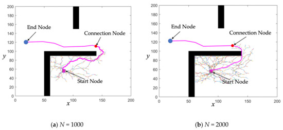
Figure 17.
Assembly paths planned with different N of Case Study 1.
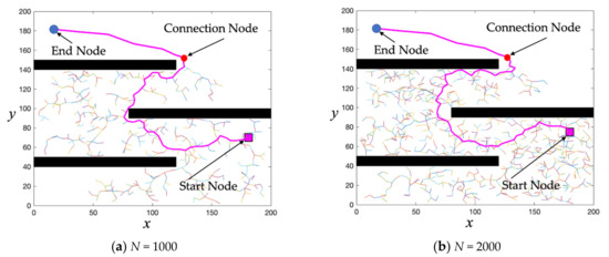
Figure 18.
Assembly paths planned with different N of Case Study 2.
Figure 17 and Figure 18 show that path planning using the PPR algorithm is completed even when the number of sampling points is small. Moreover, as the number of sampling points increases, the exploring path segment becomes asymptotically optimal. Since the weight of the prior path is greater than that of the exploring path, the connection node gradually approaches the end node, and the prior path segment of the final path is asymptotically the shortest.
4.2. The Comparison of Results of RRT * and PPR
- (1)
- The comparison of average values of results
The paths planned by using the two algorithms are random due to the small number of sampling points, resulting in different results for each algorithm when planning the same path. Therefore, the number of sampling points, the path length, and the running time when the path is successfully planned for the first time are calculated for the two algorithms, and the average values of 100 sets of planning results of Case Study 1 are compared, as shown in Table 1.

Table 1.
Average values of the planning results obtained by the rapidly exploring random tree star (RRT *) algorithm and path planning algorithm based on prior path reuse (PPR).
Table 1 shows that the average number of sampling points of the PPR algorithm is only 1/4 that of the RRT * algorithm in path planning, and the path length and running time of the PPR algorithm are also less than those of the RRT * algorithm.
- (2)
- The comparison of success rates of results
In the virtual assembly of complex products, the start positions of the parts are different; thus, 50 starting points are randomly generated in the configuration space, and the assembly path for each starting point is planned by using the RRT * algorithm and the PPR algorithm. The number of successful plans with different maximum numbers of sampling points is taken as the success rate of each algorithm, as shown in Figure 19. When the success rate equals 1, it means that every starting point finds an assembly path successfully.
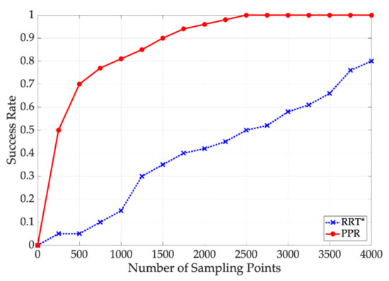
Figure 19.
Success rate of the PPR algorithm and the RRT * algorithm of Case Study 1.
Figure 19 shows that the success rate of both algorithms increases as the number of sampling points increases. However, the success rate of the PPR algorithm is much larger than that of the RRT * algorithm when the maximum number of sampling points is small.
The curves in Figure 19 show the relationship between the maximum number of sampling points and the success rate. For example, when the maximum number of sampling points is 500, the success rates of PPR and RRT * are about 0.7 and 0.05, which means 0.7 and 0.05 of starting points find their assembly paths by performing PPR and RRT *, respectively. The number of sampling points need to be 12,000 and 2500 at least by RRT * and PPR to make the success rates become 1.
- (3)
- The comparison of the minimum number of sampling points
The above-mentioned path planning results presented in Table 2 show that the minimum number of sampling points and the calculation time required by the PPR algorithm are much smaller than those of the RRT * algorithm, which verifies the effectiveness of the PPR algorithm.
Table 2.
Comparison of the planning results obtained by the RRT * and PPR algorithms.
5. Conclusions
The large number of parts in a complex product makes the repetition of path planning inevitable, which leads to low assembly efficiency. To solve this problem, this paper proposes a rapid APP method by reusing the prior path based on the RRT * algorithm.
First, an assembly path is divided into three phases to reduce the difficulty of reuse, and the logistics phase of the path is taken as the main object of reuse. Second, the path planning of a part in the assembly space is converted to searching for a non-interference path in the configuration space. Third, a dual-tree fusion strategy and the optimal path selection strategy are designed to implement the PPR algorithm. Finally, the PPR algorithm and the RRT * algorithm are compared by example analysis.
The examples and comparison list the comparison of results with different numbers of sampling points and ones with of RRT * and PPR, which conclude the advantage of the proposed method as follows: (1) The results with different numbers of sampling points show that the PPR algorithm is completed when the number of sampling points is small, which means the proposed method performs well in the case of small sampling sizes; (2) the results of RRT * and PPR show that if the maximum number of sampling points is small, the success rate of path planning by using the PPR algorithm is much greater than that of the RRT * algorithm; (3) the results of path planning with one and multiple start points show that the planning time and the number of sampling points of the PPR algorithm are much smaller than those of the RRT * algorithm, which means that the proposed method performs much better than the RRT * algorithm.
Future work will focus on the application of the PPR algorithm on a dynamic environment and the situation which is the prior path is interrupted by moving obstacles. The improvement of the algorithm efficiency is a next research direction. What is more, the method in this paper has been decided to be conducted in other realms, and more applications will be given in the future research.
Author Contributions
Methodology, G.Y. and Y.C.; investigation, G.Y. and H.H.; software and validation, C.Z. and H.H.; writing—original draft preparation, C.Z. and H.H.; writing—review and editing, G.Y. and Y.C. All authors have read and agreed to the published version of the manuscript.
Funding
This research was funded by the National Key Research and Development Program of China, grant number 2018YFB1701300, the National Natural Science Foundation of China, grant number 51875515, the Key Research and Development Program of Zhejiang Province, grant number 2020C0409, and the Science and Technology Project of Beijing, grant number Z191100001419014.
Institutional Review Board Statement
Not applicable.
Informed Consent Statement
Not applicable.
Data Availability Statement
The data presented in this study are available on request from the corresponding author.
Conflicts of Interest
The authors declare no conflict of interest.
References
- Qiu, C.; Zhou, S.; Liu, Z.; Gao, Q.; Tan, J. Digital assembly technology based on augmented reality and digital twins: A review. Virtual Real. Intell. Hardw. 2019, 1, 597–610. [Google Scholar] [CrossRef]
- Yi, Y.; Yan, Y.; Liu, X.; Ni, Z.; Feng, J.; Liu, J. Digital twin-based smart assembly process design and application framework for complex products and its case study. J. Manuf. Syst. 2020. [Google Scholar] [CrossRef]
- Li, T.; Lockett, H.; Lawson, C. Using requirement-functional-logical-physical models to support early assembly process planning for complex aircraft systems integration. J. Manuf. Syst. 2020, 54, 242–257. [Google Scholar] [CrossRef]
- Wallis, R.; Erohin, O.; Klinkenberg, R.; Deuse, J.; Stromberger, F. Data Mining-supported Generation of Assembly Process Plans. Procedia CIRP 2014, 23, 178–183. [Google Scholar] [CrossRef]
- Bilberg, A.; Malik, A.A. Digital twin driven human–robot collaborative assembly. CIRP Ann. 2019, 68, 499–502. [Google Scholar] [CrossRef]
- Maset, E.; Scalera, L.; Zonta, D.; Alba, I.M.; Crosilla, F.; Fusiello, A. Procrustes analysis for the virtual trial assembly of large-size elements. Robot. Comput. Integr. Manuf. 2020, 62, 101885. [Google Scholar] [CrossRef]
- Jin, X.; Zhang, T.; Yang, H. An Analysis of the Assembly Path Planning of Decelerator Based on Virtual Technology. Phys. Procedia 2012, 25, 170–175. [Google Scholar] [CrossRef][Green Version]
- Yang, Q.; Wu, D.L.; Zhu, H.M.; Bao, J.S.; Wei, Z.H. Assembly operation process planning by mapping a virtual assembly simulation to real operation. Comput. Ind. 2013, 64, 869–879. [Google Scholar] [CrossRef]
- Channarong, T.; Suthep, B. Virtual reality barrel shaft design and assembly planning accompany with CAM. Procedia Manuf. 2019, 30, 677–684. [Google Scholar] [CrossRef]
- Müller, R.; Hörauf, L.; Vette, M.; Speicher, C. Planning and Developing Cyber-physical Assembly Systems by Connecting Virtual and Real Worlds. Procedia CIRP 2016, 52, 35–40. [Google Scholar] [CrossRef]
- Müller, R.; Vette, M.; Hörauf, L.; Speicher, C. Consistent data Usage and Exchange Between Virtuality and Reality to Manage Complexities in Assembly Planning. Procedia CIRP 2016, 44, 73–78. [Google Scholar] [CrossRef]
- Ong, S.K.; Pang, Y.; Nee, A.Y.C. Augmented Reality Aided Assembly Design and Planning. CIRP Ann. 2007, 56, 49–52. [Google Scholar] [CrossRef]
- Dalvi, S.D. Optimization of Assembly Sequence Plan Using Digital Prototyping and Neural Network. Procedia Technol. 2016, 23, 414–422. [Google Scholar] [CrossRef]
- Ghandi, S.; Masehian, E. Review and taxonomies of assembly and disassembly path planning problems and approaches. Comput. Aided Des. 2015, 67, 58–86. [Google Scholar] [CrossRef]
- Ghandi, S.; Masehian, E. Assembly sequence planning of rigid and flexible parts. J. Manuf. Syst. 2015, 36, 128–146. [Google Scholar] [CrossRef]
- Lelyukhin, V.; Kolesnikova, O. Approach to Determining Order of Production of Parts and Assembly Units of Engineering Products in Production Process Planning. Procedia Eng. 2017, 206, 1515–1521. [Google Scholar] [CrossRef]
- Chen, R.S.; Lu, K.Y.; Yu, S.C. A hybrid genetic algorithm approach on multi-objective of assembly planning problem. Eng. Appl. Artif. Intell. 2002, 15, 447–457. [Google Scholar] [CrossRef][Green Version]
- Pellegrinelli, S.; Pedrocchi, N.; Tosatti, L.M.; Fischer, A.; Tolio, T. Multi-robot spot-welding cells for car-body assembly: Design and motion planning. Robot. Comput. Integr. Manuf. 2017, 44, 97–116. [Google Scholar] [CrossRef]
- Hui, W.; Dong, X.; Guanghong, D.; Linxuan, Z. Assembly planning based on semantic modeling approach. Comput. Ind. 2007, 58, 227–239. [Google Scholar] [CrossRef]
- Wang, H.; Rong, Y.; Xiang, D. Mechanical assembly planning using ant colony optimization. Comput. Aided Des. 2014, 47, 59–71. [Google Scholar] [CrossRef]
- Hadj, R.B.; Belhadj, I.; Trigui, M.; Aifaoui, N. Assembly sequences plan generation using features simplification. Adv. Eng. Softw. 2018, 119, 1–11. [Google Scholar] [CrossRef]
- Pan, W.; Wang, Y.; Chen, X.D. Domain knowledge based non-linear assembly sequence planning for furniture products. J. Manuf. Syst. 2018, 49, 226–244. [Google Scholar] [CrossRef]
- Morato, C.; Kaipa, K.N.; Gupta, S.K. Improving assembly precedence constraint generation by utilizing motion planning and part interaction clusters. Comput. Aided Des. 2013, 45, 1349–1364. [Google Scholar] [CrossRef]
- Ladeveze, N.; Fourquet, J.Y.; Puel, B. Interactive path planning for haptic assistance in assembly tasks. Comput. Graph. 2010, 34, 17–25. [Google Scholar] [CrossRef]
- Yan, Y.; Poirson, E.; Bennis, F. An interactive motion planning framework that can learn from experience. Comput. Aided Des. 2015, 59, 23–38. [Google Scholar] [CrossRef]
- Sierla, S.; Kyrki, V.; Aarnio, P.; Vyatkin, V. Automatic assembly planning based on digital product descriptions. Comput. Ind. 2018, 97, 34–46. [Google Scholar] [CrossRef]
- Kardos, C.; Váncza, J. Application of Generic CAD Models for Supporting Feature Based Assembly Process Planning. Procedia CIRP 2018, 67, 446–451. [Google Scholar] [CrossRef]
- Michniewicz, J.; Reinhart, G.; Boschert, S. CAD-Based Automated Assembly Planning for Variable Products in Modular Production Systems. Procedia CIRP 2016, 44, 44–49. [Google Scholar] [CrossRef]
- Qian, C.; Zhang, Y.; Jiang, C.; Pan, S.; Rong, Y. A real-time data-driven collaborative mechanism in fixed-position assembly systems for smart manufacturing. Robot. Comput. Integr. Manuf. 2020, 61, 101841. [Google Scholar] [CrossRef]
- Hassan, S.; Yoon, J. Haptic assisted aircraft optimal assembly path planning scheme based on swarming and artificial potential field approach. Adv. Eng. Softw. 2014, 69, 18–25. [Google Scholar] [CrossRef]
- Lee, D.; Kim, M.Y.; Cho, H. Path planning for micro-part assembly by using active stereo vision with a rotational mirror. Sens. Actuators A Phys. 2013, 193, 201–212. [Google Scholar] [CrossRef]
- Wei, H.X.; Mao, Q.; Guan, Y.; Li, Y.D. A centroidal Voronoi tessellation based intelligent control algorithm for the self-assembly path planning of swarm robots. Expert Syst. Appl. 2017, 85, 261–269. [Google Scholar] [CrossRef]
- Gaisbauer, F.; Lehwald, J.; Agethen, P.; Otto, M.; Rukzio, E. A Motion Reuse Framework for Accelerated Simulation of Manual Assembly Processes. Procedia CIRP 2018, 72, 398–403. [Google Scholar] [CrossRef]
- Li, B.; Liu, H.; Su, W. Topology optimization techniques for mobile robot path planning. Appl. Soft Comput. 2019, 78, 528–544. [Google Scholar] [CrossRef]
- Song, P.C.; Pan, J.S.; Chu, S.C. A parallel compact cuckoo search algorithm for three-dimensional path planning. Appl. Soft Comput. 2020, 94, 106443. [Google Scholar] [CrossRef]
- Sun, Z.; Shao, Z.F.; Li, H. An eikonal equation based path planning method using polygon decomposition and curve evolution. Def. Technol. 2019. [Google Scholar] [CrossRef]
- Sung, I.; Choi, B.; Nielsen, P. On the training of a neural network for online path planning with offline path planning algorithms. Int. J. Inf. Manag. 2020. [Google Scholar] [CrossRef]
- Heinemann, T.; Riedel, O.; Lechler, A. Generating Smooth Trajectories in Local Path Planning for Automated Guided Vehicles in Production. Procedia Manuf. 2019, 39, 98–105. [Google Scholar] [CrossRef]
- Terh, S.H.; Cao, K. GIS-MCDA based cycling paths planning: A case study in Singapore. Appl. Geogr. 2018, 94, 107–118. [Google Scholar] [CrossRef]
- Zhao, Y.; Zheng, Z.; Liu, Y. Survey on computational-intelligence-based UAV path planning. Knowl. Based Syst. 2018, 158, 54–64. [Google Scholar] [CrossRef]
- Jain, G.; Yadav, G.; Prakash, D.; Shukla, A.; Tiwari, R. MVO-based path planning scheme with coordination of UAVs in 3-D environment. J. Comput. Sci. 2019, 37, 101016. [Google Scholar] [CrossRef]
- Li, K.; Ge, F.; Han, Y.; Wang, Y.a.; Xu, W. Path planning of multiple UAVs with online changing tasks by an ORPFOA algorithm. Eng. Appl. Artif. Intell. 2020, 94, 103807. [Google Scholar] [CrossRef]
- Mahmud, M.S.A.; Abidin, M.S.Z.; Mohamed, Z.; Rahman, M.K.I.A.; Iida, M. Multi-objective path planner for an agricultural mobile robot in a virtual greenhouse environment. Comput. Electron. Agric. 2019, 157, 488–499. [Google Scholar] [CrossRef]
- Kavraki, L.E.; Svestka, P. Probabilistic roadmaps for path planning in high-dimensional configuration spaces. IEEE Trans. Robot. Autom. 1996, 12, 566. [Google Scholar] [CrossRef]
- Elbanhawi, M.; Simic, M. Sampling-Based Robot Motion Planning: A Review. IEEE Access 2014, 2, 56–77. [Google Scholar] [CrossRef]
- Wang, W.; Deng, H.; Wu, X. Path planning of loaded pin-jointed bar mechanisms using Rapidly-exploring Random Tree method. Comput. Struct. 2018, 209, 65–73. [Google Scholar] [CrossRef]
- Yuan, C.; Liu, G.; Zhang, W.; Pan, X. An efficient RRT cache method in dynamic environments for path planning. Robot. Auton. Syst. 2020, 131, 103595. [Google Scholar] [CrossRef]
- Cao, X.; Zou, X.; Jia, C.; Chen, M.; Zeng, Z. RRT-based path planning for an intelligent litchi-picking manipulator. Comput. Electron. Agric. 2019, 156, 105–118. [Google Scholar] [CrossRef]
- Qian, K.; Liu, Y.; Tian, L.; Bao, J. Robot path planning optimization method based on heuristic multi-directional rapidly-exploring tree. Comput. Electr. Eng. 2020, 85, 106688. [Google Scholar] [CrossRef]
- Li, Y.; Wei, W.; Gao, Y.; Wang, D.; Fan, Z. PQ-RRT*: An improved path planning algorithm for mobile robots. Expert Syst. Appl. 2020, 152, 113425. [Google Scholar] [CrossRef]
- Chao, N.; Liu, Y.K.; Xia, H.; Peng, M.J.; Ayodeji, A. DL-RRT* algorithm for least dose path Re-planning in dynamic radioactive environments. Nucl. Eng. Technol. 2019, 51, 825–836. [Google Scholar] [CrossRef]
- Xiong, J.; Hu, Y.M.; Wu, B.; Duan, X.K. Minimum-cost rapid-growing random trees for segmented assembly path planning. Int. J. Adv. Manuf. Technol. 2015, 77, 1043–1055. [Google Scholar] [CrossRef]
- Rosell, J.; Iniguez, P. Path planning using Harmonic Functions and Probabilistic Cell Decomposition. In Proceedings of the 2005 IEEE International Conference on Robotics and Automation, Barcelona, Spain, 18–22 April 2005; pp. 1803–1808. [Google Scholar] [CrossRef]
- Borenstein, J.; Koren, Y. The vector field histogram-fast obstacle avoidance for mobile robots. IEEE Trans. Robot. Autom. 1991, 7, 278–288. [Google Scholar] [CrossRef]


Publisher’s Note: MDPI stays neutral with regard to jurisdictional claims in published maps and institutional affiliations. |
© 2021 by the authors. Licensee MDPI, Basel, Switzerland. This article is an open access article distributed under the terms and conditions of the Creative Commons Attribution (CC BY) license (http://creativecommons.org/licenses/by/4.0/).