Abstract
Over the past decade, deep learning-based computer vision methods have been shown to surpass previous state-of-the-art computer vision techniques in various fields, and have made great progress in various computer vision problems, including object detection, object segmentation, face recognition, etc. Nowadays, major IT companies are adding new deep-learning-based computer technologies to edge devices such as smartphones. However, since the computational cost of deep learning-based models is still high for edge devices, research is being actively carried out to compress deep learning-based models while not sacrificing high performance. Recently, many lightweight architectures have been proposed for deep learning-based models which are based on low-rank approximation. In this paper, we propose an alternating tensor compose-decompose (ATCD) method for the training of low-rank convolutional neural networks. The proposed training method can better train a compressed low-rank deep learning model than the conventional fixed-structure based training method, so that a compressed deep learning model with higher performance can be obtained in the end of the training. As a representative and exemplary model to which the proposed training method can be applied, we propose a rank-1 convolutional neural network (CNN) which has a structure alternatively containing 3-D rank-1 filters and 1-D filters in the training stage and a 1-D structure in the testing stage. After being trained, the 3-D rank-1 filters can be permanently decomposed into 1-D filters to achieve a fast inference in the test time. The reason that the 1-D filters are not being trained directly in 1-D form in the training stage is that the training of the 3-D rank-1 filters is easier due to the better gradient flow, which makes the training possible even in the case when the fixed structured network with fixed consecutive 1-D filters cannot be trained at all. We also show that the same training method can be applied to the well-known MobileNet architecture so that better parameters can be obtained than with the conventional fixed-structure training method. Furthermore, we show that the 1-D filters in a ResNet like structure can also be trained with the proposed method, which shows the fact that the proposed method can be applied to various structures of networks.
1. Introduction
Deep learning-based computer vision shows good performance in various computer vision areas such as image segmentation [1,2], image synthesis [3], facial recognition [4], classification [5], person re-identification [6], and object detection [7,8]. However, in spite of the remarkable achievements in difficult computer vision tasks, conventional deep convolutional neural networks (CNNs) use a high number of parameters which limits their use on devices with limited resources such as smartphones, embedded systems, etc. Even though it has been known that there exist a lot of redundancy between the parameters and the feature maps in deep models, over-parametrized CNN models are used due to the reason that over-parametrization makes the training of the network easier as has been shown in the experiments in [9]. The reason for this phenomenon is believed to be due to a better gradient flow in over-parametrized networks.
Meanwhile, it has been shown in [10] that even with the use of regularization methods, there still exists excessive capacity in trained networks, which again implies the fact that the redundancy between the parameters is still large. Therefore, many researches focus on finding a better network structure so that the parameters can be expressed in a structured subspace with smaller number of coefficients. The research topic on compressing large-scale deep learning models is increasing in importance as it is necessary to use compressed deep learning models in edge devices such as smartphones and IoT devices. While early works focused on compressing the parameters of pre-trained large scale deep learning models [11,12,13,14,15,16,17,18,19,20,21,22], studies are also actively under way to limit the number of parameters by proposing small networks in the first place [23,24,25,26,27,28,29,30,31,32,33,34,35,36,37]. Most recently, researches have prevailed on how to efficiently use these compressed models on edge devices [38,39,40,41]. We will provide a detailed overview of these research trends in Section 2.
In this paper, we propose a training method for the training of low-rank convolutional neural networks, which we call the alternating tensor compose-decompose (ATCD) method. The proposed training method can better train compressed low rank models than existing training methods, thus obtaining a compressed deep learning model with higher performance. In general, when training deep learning models, the same structure of the neural network is used during the training and the testing stages. Conventional tensor decomposing networks are trained with the fixed-structure based training method, i.e., they are trained in the decomposed form. We call the conventional training method the fixed-structure based training method. In comparison, the proposed training method do not use a fixed structure of neural network in the training stage, but allows the tensors to be alternatingly composed and decomposed so that a better gradient flow can flow through the tensors in the backpropagation step. This better gradient flow results in better parameter values than with conventional training method so that the compressed model can achieve a higher performance. As an example of the proposed training method, we apply it to the rank-1 CNN, where the rank-1 CNN is iteratively and alternatingly composed into a 3-D rank-1 CNN structure and decomposed into 1-D vectors in the training stage, where the 3-D rank-1 filters are constructed by the outer products of the 1-D vectors. The number of parameters in the 3-D rank-1 filters are the same as in the 3-D filters in standard CNNs, allowing a good gradient flow in the backpropagation stage. The difference with the backpropagation stage in standard CNNs is that the gradient flow flows also through the 1-D vectors from which the 3-D rank-1 filters are constructed, updating the parameters in the 1-D vectors also. After the backpropagation step, the 3-D filters lose their rank-1 property. However, at the next composition step, the parameters in the 3-D filters are updated again by the outer product operation to be projected onto the rank-1 subspace. By iterating this two-step update, all the 3-D filters in the network are trained to minimize the loss function while maintaining their rank-1 property. This is different from approaches which try to approximate the trained filters by low rank approximation after the training has been finished, e.g., like the low rank approximation in [14] or from approaches which use the same fixed CNN structure both in the training and the testing stages. The composition operation is included in the training phase in our network, which directs the parameter update in a different direction from that of standard CNNs, directing the solution to live on a rank-1 subspace.
In the testing phase, we do not need the tensor composing stage anymore, and the 3-D rank-1 filters can be permanently decomposed into 1-D filters. So in the testing stage, the rank-1 CNN is now reconstructed into a 1-D rank-1 CNN structure with the trained 1-D vectors used as the 1-D filters. So the rank-1 CNN has the same accuracy as the 3-D rank-1 CNN, but has the same inference speed as the 1-D rank-1 CNN, i.e., the inference speed is exactly the same as that of the Flattened network. Moreover, with the proposed method, the network can be trained even in the case when the Flattened network cannot be trained at all. In other words, the proposed training method can be applied to train networks with very limited gradient paths due to the low rank property which cannot be trained with conventional training methods.
We also show how the same training method can be applied to the well-known MobileNet. We first show how the channel-wise filters can be expressed as a linear combination of low rank filters, and then show how the proposed alternating tensor compose-decompose (ATCD) training method can be applied to the training of the low rank filters. The low rank filters are composed into the MobileNet structure again at the end of the training. Thereby, better parameters are obtained than with conventional training with fixed MobileNet structure.
2. Related Works
In this section, we summarize the works related to our work in accordance with the evolving trend of research in this field. However, it should be noted that our work is somewhat unique and different from the related works in the aspect that we did not compress the parameters of pre-trained models or propose a new model architecture, but propose a new training method to train existing factorized structures to have better parameter values.
2.1. Works on Compressing the Parameters of Pre-Trained CNNs
Early works on compressing the CNN focused on how to compress the pre-trained parameters without loss of information. As has been well summarized in [42], researches on the compression of deep models can be categorized into works which try to eliminate unnecessary weight parameters [11,12], works which try to compress the parameters by projecting them onto a low rank subspace [13,14,15,16], and works which try to group similar parameters into groups and represent them by representative features [18,19,20,21,22]. These works follow the common framework of first training the original uncompressed CNN model by back-propagation to obtain the uncompressed parameters, and then trying to find a compressed expression for these parameters to construct a new compressed CNN model.
2.2. Works on Designing a Compressed Model
Compared to the works of compressing the pre-trained parameters, researches which try to restrict the number of parameters in the first place by proposing small networks are also actively in progress. However, as mentioned above, the reduction in the number of parameters changes the gradient flow, so the networks have to be designed carefully to achieve a trained network with good performance. For example, MobileNets [23] and Xception networks [24] use depthwise separable convolution filters, while the SqueezeNet [25] uses a bottleneck approach to reduce the number of parameters. MobileNet was modified in version 2 model using inverted residuals [26]. Recently, Google announced the EfficientNet [27] which scales up the MobileNet and the ResNet to obtain a new family of efficient CNN models, while CondenseNet [28] and ShuffleNet [29] are using group convolutions to reduce the number of convolutions. Other models use 1-D filters to reduce the size of networks such as the highly factorized Flattened network [30], or the models in [31] where 1-D filters are used together with other filters of different sizes. Recently, Google’s Inception model has also adopted 1-D filters in version 4 [43]. One difficulty in using 1-D filters is that 1-D filters are not easy to train, and therefore, they are used only partially like in the Google’s Inception model, or in the models in [31] etc., except for the Flattened network which is constituted of consecutive 1-D filters only. However, only three layers of 1-D filters are used in the experiments in [30], which is maybe due to the difficulty of training 1-D filters with many layers.
Until now, all the efficient neural network architectures have been developed manually by human experts. Though still in the early stage, there are researches ongoing to automatically searching for architectures that are efficient and satisfy the resource or computation constraints [32,33,34,35,36,37]. However, it is known that such an automatic neural architecture search is extremely difficult, and therefore, in practice, the manually well-designed architectures are still widely used.
2.3. Works on Edge AI
Now that many efficient and compressed CNN architectures have been proposed, many researchers and major IT companies are focusing on how to shift these compression models to edge devices as customers spend more time on mobile devices [38,39,40,41,44,45,46,47,48]. Particularly, in [38], Eshratifar et al. propose an efficient training for intelligent mobile cloud computing services, while in [39] Li et al. proposed how to accelerate the inference in DNN via edge computing. In [40], a deep learning architecture for intelligent mobile cloud computing services called BottleNet is proposed, which reduces the feature size needed to be sent to the cloud. Furthermore, Bateni and Lie propose a timing-predictable runtime system that is able to guarantee deadlines of DNN workloads via efficient approximation [41]. It is believed that Edge AI research and algorithms on both commercial and academic laboratories are expected to be very active in the next three to five years.
3. Preliminaries for the Proposed Method
The following works have to be understood to understand the proposed method. The work of bilateral-projection based 2-D principal component analysis (B2DPCA) gave us the insight for bilateral filters and the tensor compose-decompose procedure, which we utilized to train the rank-1 Net.
3.1. Bilateral-Projection Based 2DPCA
In [49], a bilateral-projection based 2-D principal component analysis (B2DPCA) has been proposed, which minimizes the following energy functional:
where is the two dimensional image, and are the left- and right- multiplying projection matrices, respectively, and is the extracted feature matrix for the image . The optimal projection matrices and are simultaneously constructed, where projects the column vectors of to a subspace, while projects the row vectors of to another one. It has been shown in [49], that the advantage of the bilateral projection over the unilateral-projection scheme is that can be represented effectively with smaller number of coefficients than in the unilateral case, i.e., a small-sized matrix can well represent the image . This means that the bilateral-projection effectively removes the redundancies among both rows and columns of the image. Furthermore, since
it can be seen that the components of are the 2-D projections of the image onto the 2-D planes , , … made up by the outer products of the column vectors of and . The 2-D planes have a rank of one, since they are the outer products of two 1-D vectors. Therefore, the fact that can be well represented by a small-sized also implies the fact that can be well represented by a few rank-1 2-D planes, i.e., only a few 1-D vectors , where and .
In the case of (1), the learned 2-D planes try to minimize the loss function
i.e., try to learn to best approximate . A natural question arises, if good rank-1 2-D planes can be obtained to minimize other loss functions too, e.g., loss functions related to the image classification problem, such as
where denotes the true classification label for a certain input image , and is the output of the network constituted by the outer products of the column vectors in the learned matrices and . In this paper, we extend this case to the rank-1 3-D filter case, where the rank-1 3-D filter is constituted as the outer product of three column vectors from three different learned matrices, and show that good parameters can be learned for the image classification task. Furthermore, these learned rank-1 3-D filters can be decomposed into rank-1 1-D filters for fast inference speed.
3.2. Flattened Convolutional Neural Networks
In [30], the ‘Flattened CNN’ has been proposed for fast feed-forward execution by separating the conventional 3-D convolution filter into three consecutive 1-D filters. The 1-D filters sequentially convolve the input over different directions, i.e., the lateral, horizontal, and vertical directions. Figure 1 shows the network structure of the Flattened CNN. The Flattened CNN uses the same network structure in both the training and the testing phases. This is in comparison with our proposed model, where we use a different network structure in the training phase as will be seen later.
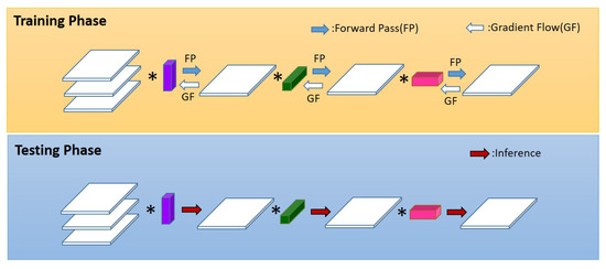
Figure 1.
The structure of the Flattened network. The same network structure of sequential use of 1-D filters is used in the training and testing phases. Here, ∗ denotes the convolution operator.
However, the consecutive use of 1-D filters in the training phase makes the training difficult. This is due to the fact that the gradient path becomes longer than in normal CNN, and therefore, the gradient flow vanishes faster while the error accumulates more. Another reason is that the reduction in the number of parameters causes a gradient flow different from that of the standard CNN, which is more difficult to find an appropriate solution for the parameters. This fact coincides with the experiments in [9] which show that the gradient flow in a network with small number of parameters cannot find good parameters. Therefore, a particular weight initialization method has to be used together with this setting. Furthermore, in [30], the networks in the experiments have only three layers of convolution, which is maybe due to the fact of the difficulty in training networks with more layers.
4. Application of the Proposed Training Method to the Rank-1 CNN
As an example of how the tensor composing-decomposing method can be applied to train low-rank CNNs, we apply the proposed training method to the rank-1 CNN which is composed of mere rank-1 convolutional filters. In comparison with other CNN models which use 1-D rank-1 filters, we propose the use of 3-D rank-1 filters() in the training stage, where the 3-D rank-1 filters are constructed by the outer product of three 1-D vectors, say , , and :
This is an extension of the 2-D rank-1 planes used in the B2DPCA, where the 2-D planes are constructed by . Figure 2 shows the training and the testing phases of the proposed method. The structure of the proposed network is different for the training phase and the testing phase. In comparison with the Flattened network (Figure 1), in the training phase, the gradient flow first flows through the 3-D rank-1 filters and then through the 1-D vectors. Therefore, the gradient flow is different from that of the Flattened network resulting in a different and better solution of parameters in the 1-D vectors. The solution can be obtained even in large networks with the proposed method, for which the gradient flow in the Flattened network cannot obtain a solution at all. Furthermore, at test time, i.e., at the end of optimization, we can use the 1-D vectors directly as 1-D filters in the same manner as in the Flattened network, resulting in the same inference speed and number of operations as the Flattened network (Figure 2).
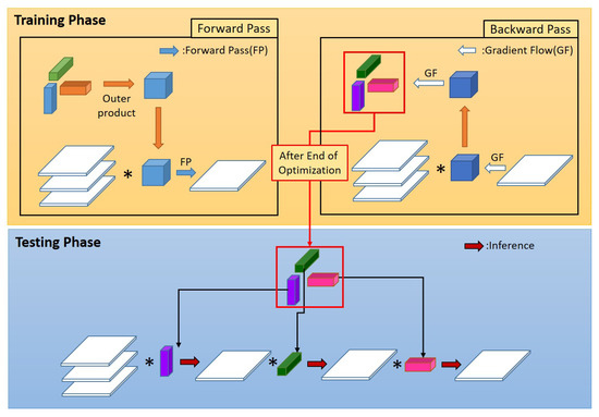
Figure 2.
Proposed rank-1 neural network with different network structures in training and testing phases. Here, ∗ denotes the convolution operator.
4.1. Construction of the 3-D Rank-1 Filters
We first observe that a 2-D convolution can be seen as shifting inner products, where each component at position of the output matrix is computed as the inner product of a 2-D filter and the image patch centered at :
If is constructed by the outer product of two 1-D vectors and , i.e., , then becomes a 2-D rank-1 filter. In this case, it can be observed that
As has been explained in the case of B2DPCA, since is multiplied to the rows of , tries to extract the features from the rows of which can minimize the loss function. That is, searches the rows in all patches for some common features which can reduce the loss function, while looks for the features in the columns of the patches. In analogy to the B2DPCA, this bilateral projection removes the redundancies among the rows and columns in the 2-D filters.
In convolutional neural networks, the input and the convolutional filter are both three dimensional, where the third dimension refers to the depth of the input, i.e., the numer of input channels. In this case, the 3-D rank-1 filter is constructed by the outer product of three 1-D vectors , , and ,
where the length of is the same as the depth of the input . In analogy to the B2DPCA, the 3-D rank-1 filters which are learned by the three dimensional multilateral projection will have less redundancies among the rows, columns, and the channels than the normal 3-D filters in standard CNNs.
The three dimensional convolution of the 3-D rank-1 filter and can be expressed by the sum of channel-wise 2-D convolutions. Let denote the i’s 3-D rank-1 filter that results in the i’s output channel , and the 2-D rank-1 filter that relates with , which is constructed by the outer product of two 1-D vectors and . We construct a rank-1 2-D filter for each output channel ,
The total number of 2-D filters is , where q is the number of output channels. Then, the 3-D rank-1 filters can be constructed by
Furthermore, let denote the j’s 2-D channel in . Then the 3-D convolution which results in the i’s output channel can be expressed as
where ∗ and ⊛ denote the 3-D and the 2-D convolution operations, respectively, and refers to the j’s component of the vector . Figure 3 visualizes how the 3-D rank-1 filters are constructed and how they convolve with the 2-D channels in .
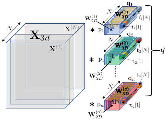
Figure 3.
Constitution of the 3-D rank-1 filters in the training phase. The 3-D filters that are convolved with the 3-D input are constructed by the outer products of the 2-D filters and the 1-D filters , respectively, where the 2-D filters are again constructed by the outer products of the 1-D filters and according to Equation (9).
As explained above, at test time, we can use the trained 1-D vectors as the 1-D filters, so that in the test time only 1-D convolutions are used. As has been shown in [30], when using only 1-D convolutions, the number of operations reduces to
instead of
where and are the width and height of the input feature map, respectively, is the number of output channels, and and are the width and height of the filter.
4.2. Training Process
Figure 4 explains the training process with the proposed network structure in detail. At every epoch of the training phase, we first take the outer product of the three 1-D vectors , , and . Then, we assign the result of the outer product to the weight values of the 3-D convolution filter, i.e., for every weight value in the 3-D convolution filter , we assign
where, correspond to the 3-D coordinates in , the 3-D domain of the 3-D convolution filter . Since the matrix constructed by the outer product of vectors has always a rank of one, the 3-D convolution filter is a rank-1 filter.
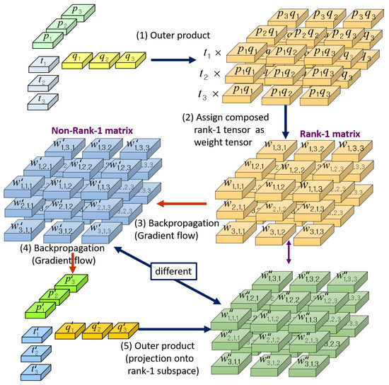
Figure 4.
Steps in the training phase of the proposed rank-1 network.
During the back-propagation phase, every weight value in will be updated by
where denotes the gradient of the loss function L with respect to the weight , and is the learning rate. In standard convolutional neural networks, in (15) is the final updated weight value at each update step. However, the updated filter normally is not a rank-1 filter. This is due to the fact that the update in (15) is done in the direction which considers only the minimizing of the loss function and not the rank of the filter.
With the proposed training network structure, we take a further update step, i.e., we update the 1-D vectors , , and :
Here, , , and can be calculated as
At the next feed forward step in the back-propagation, an outer product of the updated 1-D vectors , , and is taken to concatenate them back into a 3-D convolution filter , which we call the tensor composing step:
where
As the outer product of 1-D vectors always results in a rank-1 filter, is a rank-1 filter as compared with which is not. Comparing (15) with (22), we get
Therefore, we can say that is the incremental update vector which projects back onto the rank-1 subspace. The use of rank-1 filters are not constrained to replace the filters in the standard CNN structure but can also replace the full-rank filters in ResNet or DenseNet-like architectures. In this case, the rank-1 filters can also reduce the parameters and accelerate the inference speed in ResNet or DenseNet architectures.
5. Application of the Proposed Training Method to the MobileNet
Here, we show that the proposed rank-1 network training method can also be applied to train the well-known MobileNet (version 1). However, the performance becomes better when the parameters are obtained by the proposed method, than when obtained by the original MobileNet type training method. The main idea of applying the proposed training method to the training of the MobileNet is that we can extend the separate 2-D filters to 3-D filters by the outer product of rank-1 2-D filters with rank-1 1-D vectors resulting in rank-1 3-D filters, train the rank-1 3-D filters with the ATCD training method, and then compress the rank-1 3-D filters back to full-rank 2-D filters. In the original version (version 1) of the MobileNet, the 2-D images are separately convolved with 2-D filters, and then are combined by convolutions. The output of a single layer of the original version of the MobileNet can be written as
where is the m’s output channel, is the j’s input channel, is the j’s filter that convolves with the j’s input channel, ⊛ is the 2-D convolution operator, and is the m’s convolution filter that produces the m’s output channel. Meanwhile, the outputs which are obtained by the convolutions of the 3-D rank-1 filters and the input channels as shown in Figure 3 become
It has to be noted that the index of in (26) is i (the index of output channels) compared to (25) where the index of is j (the index of input channels).
Now, adding an extra layer which computes the linear combinations of the outputs in (26) by convolutions with the filters , we have
After the values of and are all fixed for all m, i, and j, i.e., after they have been trained, we can arbitrarily construct the vectors and so that the entries in the vectors are assigned as follows:
By letting
the formula becomes the same as that for the Mobilenet described in (25). This means that after being training by the proposed method, we can implement the inference system also in the Mobilenet style. It has to be noticed that even though is a two dimensional rank-1 filter, since it is composed of the outer product of two 1-D vectors, the filter can have a rank of K, as the summation of K independent rank-1 filters results in a rank-K filter. As shown in the experiments, the proposed method learns better parameters due to the over-parametrization produced by the outer product into a 3-D filter, and therefore, the MobileNet constructed by the proposed rank-1 training method has a higher accuracy than that of the original MobileNet which is trained with a smaller number of parameters. Therefore, the proposed training method can contribute to obtain MobileNets with higher classification accuracies.
6. Experiments
We compared the performance of the proposed ATCD training method with the conventional fixed structure training method for the rank-1 CNN and the MobileNet on various datasets. We also compared the validation and testing accuracies with a standard full-rank CNN. We used the same number of layers for all the models, where for the fixed structured Flattened CNN we regarded the combination of the lateral, vertical, and horizontal 1-D convolutional layers as a single layer. Furthermore, we used the same numbers of input and output channels in each layer for all the models, and also the same ReLU(Rectified Linear Unit), batch normalization, and dropout operations.
Table 1, Table 2, Table 3 and Table 4 show the different structures of the models used for each dataset in the training stage. The outer product operation of the three 1-D filters , , and into a 3-D rank-1 filter is denoted as in the tables. We did not elaborate on the structures to produce the optimal performances, but only tried to make them the same for fair comparison. Furthermore, we did not use any recent structures with extra components like skip-connections, element-wise or channel-wise concatenations, multi-scale filters, such as the ResNet or DenseNet, but intentionally used simple VGG-like structures with simple consecutive convolutional filters to see only the effect of the proposed training method. However, to verify the fact that the proposed training method can be applied also to the training of rank-1 filters inside a ResNet or DenseNet structure, we further performed an experiment on the CIFAR10 dataset with the ResNet structure where we replaced all the convolutional filters with the rank-1 filters and then applied our ATCD training method.

Table 1.
Structure of convolutional neural network (CNN)1 for the MNIST dataset.
Table 2.
Structure of CNN2 for CIFAR-10 dataset.
Table 3.
Structure of CNN3 for ‘Dog and Cat’ dataset.
Table 4.
Structure of CNN4 for CIFAR-100 dataset.
The datasets that we used in the experiments were the MNIST, the CIFAR10, CIFAR100, and the ‘Dog and Cat’ datasets (https://www.kaggle.com/c/dogs-vs-cats). We used different structures for different datasets, which we denoted as CNN1, CNN2, CNN3, and CNN4 in the tables, corresponding to the MNIST, CIFAR10, CIFAR100, and ‘Dog and Cat’ datasets, respectively. The MNIST and the CIFAR-10 datasets both consisted of 60,000 images in 10 different classes, divided into 50,000 training images and 10,000 test images, where the images in the CIFAR-10 dataset were colour images of size 32 × 32, while those in the MNIST dataset were gray images of size 28 × 28. The CIFAR-100 data set consisted of 100 classes, each with 500 training and 100 test color images of size 32 × 32. The ‘Dog and Cat’ dataset contained 25,000 color images of dogs and cats of size , which we divided into 24,900 training and 100 test images for the validation test along the training. At the end of each training session, we tested the final testing accuracy of the ‘Dog and Cat’ dataset by taking the average of the 100 test images. Then, the final testing accuracy was obtained by taking the mean of 10 of such sessions. For the experiments on the MNIST, the CIFAR10, and the CIFAR100 datasets, we trained on 50,000 images, and then tested on 100 batches each consisting of 100 random test images, and calculated the overall average accuracy both for the validation along the training and for the final testing. We plotted for every training epoch the validation accuracy values in Figure 5, Figure 6, Figure 7, Figure 8 and Figure 9. The number of epochs in the figures were determined to be greater than the epochs for which the validation accuracies with the proposed model sufficiently converged, and which resulted in graphs from which it became possible to visually compare the results of the different methods. Figure 5, Figure 6, Figure 7, Figure 8 and Figure 9 show the validation accuracies for every epoch along the training process for a single training for each model. Even though it is customary to learn a model only once in deep learning, we performed multiple training sessions for each dataset, and obtained different models at the end of each training. Then, we calculated the means and the standard deviations of the different final accuracy values of the testing datasets for each trained model, and recorded them in Table 5. For the experiments on MNIST, CIFAR10, and CIFAR100 datasets, 20 training sessions were performed, and for the ’Dog and Cat’ dataset, which took a long time to train, 10 training sessions were performed to obtain the values in Table 5. The slight differences between the testing accuracies of the different models are due to the different initialization of convolutional filters and the randomness of the stochastic gradient descent-based backpropagation.
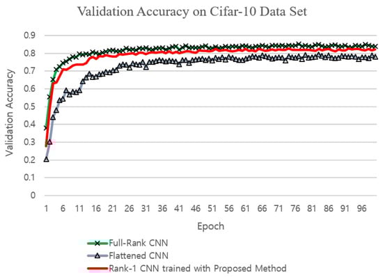
Figure 5.
Comparison of validation accuracies on the CIFAR10 dataset.
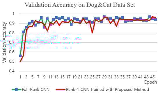
Figure 6.
Comparison of validation accuracies on the ‘Dog and Cat’ dataset.
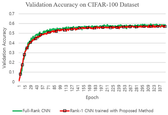
Figure 7.
Comparison of validation accuracies on the CIFAR100 dataset.
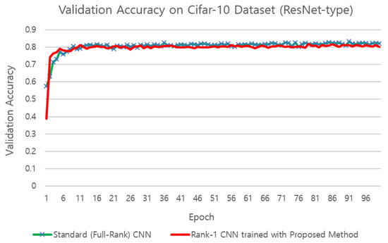
Figure 8.
Comparison of validation accuracies on the CIFAR10 dataset with the ResNet structure.
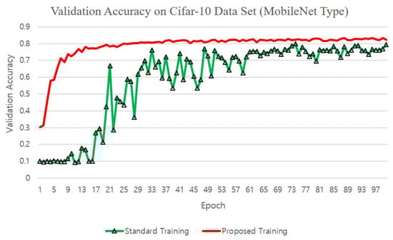
Figure 9.
Comparison of validation accuracies on the CIFAR10 dataset with the proposed and the standard training methods for the MobileNet.
Table 5.
Comparison of accuracy and inference time between the different training methods with different architectures. Mean and std. stands for average and standard deviation. The values in the inference times are the mean and the standard deviation values, respectively, where the unit is second for the average value.
The rank-1 CNN trained with the proposed training method achieved slightly larger validation and testing accuracies on the MNIST dataset than the standard full-rank CNN and the Flattened CNN trained with the conventional fixed-structure training method (Figure 10 and Table 5). This is maybe due to the fact that the MNIST dataset was in its nature a low-ranked one, for which the proposed method could find the best approximation since the proposed method constrains the filters to a low rank sub-space. With the CIFAR10 and the CIFAR100 dataset, the accuracy was slightly less than that of the standard CNN which is maybe due to the fact that the images in the CIFAR10 and the CIFAR100 datasets were of higher ranks than those in the MNIST dataset. However, the validation accuracy of the rank-1 CNN trained with the proposed method was higher than that of the Flattened CNN trained with the conventional fixed structure training method on the CIFAR10 dataset which shows the fact that the better gradient flow in the proposed training method achieves a better solution. With the CIFAR100 dataset, the Flattened CNN could not be trained by conventional fixed structure training methods due to the deep structure of the CNN4 structure. The ‘Dog and Cat’ dataset was used in the experiments to verify the validness of the proposed training method on real-sized images and on a deep structure. In this case, again the Flattened network could not be trained with the conventional fixed structure training method. This is maybe due to the limitation to produce a gradient flow in deep structures with the direct fixed 1-D structure of the Flattened CNN. The standard CNN trained with conventional training method and the proposed rank-1 CNN trained with the proposed training method achieved similar validation accuracies as can be seen in Figure 6. The validation accuracies for the CIFAR100 dataset are shown in Figure 7. Again, it can be seen that the rank-1 CNN trained with the proposed ATCD method achieved similar validation and testing accuracies to the standard CNN.
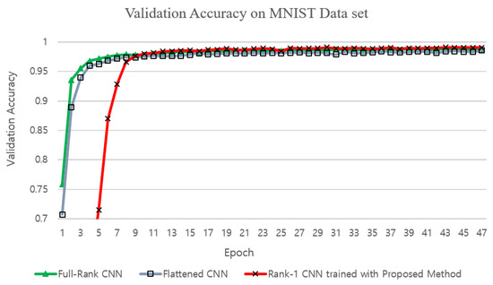
Figure 10.
Comparison of validation accuracies on the MNIST dataset.
The number of operations reduced according to (12). So, for example, for the first layer of the structure CNN3, the number of operations for the standard CNN and the rank-1 (type-1) became = 28,901,376 and = 3,512,320, respectively. Therefore, the computation operations in the first convolutional layer in the CNN3 model was about eight times more with the standard CNN. Table 6 summarizes the number of parameters for the different models and structures. We also performed experiments on the inference times for the different models on CPU and GPU environments, and recorded the values in the fifth and sixth columns in Table 5. We used Tensorflow version 0.12.1 and ran it on Window10 OS, with NVIDIA 1080Ti GPU, Intel i9 CPU and 16 GB RAM memory. It should be noted that the Flattened model and the proposed model had the same inference speed as the structures in the testing time werere the same. Compared to the reduction ratio of the number of parameters, the increase in the inference speed was not that high, which is mainly due to the fact that the Tensorflow framework was not optimized for factorized neural networks and that the loading of the image took a long time in the inference stage. We believe that in the future, the speed of factorized filtering will increase with a framework optimized for them.
Table 6.
Comparison of numbers of parameters in convolutional filters.
Figure 8 compares the validation accuracies of the networks with ResNet structures composed of standard 3-D filters and rank-1 3-D filters, respectively, where the rank-1 3-D filters were trained with the proposed training method. We used the 56-layer ResNet structure for CIFAR10 as proposed in [50], and replaced all the standard 3-D filters by rank-1 3-D filters in the ResNet in the experiments with the proposed training method. As can be seen, the rank-1 ResNet trained with the proposed method achieved similar validation accuracy to the normal ResNet, which shows that the proposed training method can be applied to diverse network structures containing low-rank filters.
Finally, Figure 9 compares the validation accuracies of the MobileNet when trained with the normal method and with the proposed training method. We used the CNN4 structure and replaced all the 3-D convolution operations with the depth-wise separable 2-D convolutions + pointwise convolutions as suggested in the MobileNet structure. It can be seen that the proposed training method could accelerate the training process and achieved a better validation accuracy than the standard training method, which is due to the intentional over-parametrization obtained by the outer product with the proposed method. Figure 11 shows the means and the positive standard deviations of the validation accuracies for different training sessions. It can be seen that the standard deviations at the early epochs of the training with the standard training method were large, while with the proposed training method the variation was not so large. However, after a long time of training, the final validation accuracies all converged to a similar value for each training session as shown by the standard deviation that decreased at the end of the training.
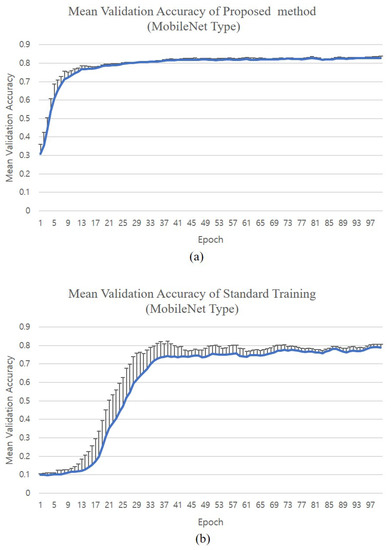
Figure 11.
Comparison of mean validation accuracies on the CIFAR10 dataset with the proposed and the standard training methods for the MobileNet. (a) Mean validation accuracies of the proposed training method (vertical bars show the positive standard deviation); (b) mean validation accuracies of the standard training method (vertical bars show the positive standard deviation).
7. Conclusions
We proposed a training method which alternatively composes and decomposes the filters in the training stage for better training of low rank filters. As an exemplary case, we showed that a rank-1 CNN can be trained with the proposed method, which cannot be trained with conventional training methods. We used 3-D rank-1 filters in convolutional neural networks in the training phase, so that the redundancy in the filters are reduced by the rank deficient property of the rank-1 filters. The proposed training method updates the 3-D filter parameters and projects them back onto the rank-1 subspace at each epoch to find good parameter values for the 1-D vectors which constitute the 3-D filters. At test time, the trained 1-D vectors can be used directly as 1-D filters which filter the image by 1-D convolution instead of the 3-D convolution for fast inference. We showed in the experiments that the accuracy performance of the rank-1 CNN is almost the same as the standard CNN while reducing the number of parameters up to about 11%, and the number of operations up to about 12% in the convolution filters compared with the standard CNN. We also showed that the proposed method can also be used in the ResNet structure and showed that the proposed training method can be utilized for a better training of the MobileNet. This suggests the possibility that the proposed rank-1 training method can also be used with diverse structures such as the ResNet or other small-sized networks, to obtain a more efficient network structure.
In this paper, we applied the proposed training method to well-known deep learning models that can be factorized. Whether the proposed training method can be applied to other complicated models still leaves much room. Combining the proposed method with the existing training method and applying it to other complex deep learning models can be an additional topic of this study. Moreover, the experimental results showed that the inference time was not reduced as much as the decrease in the number of parameters, which is due to the fact that existing deep learning frameworks are not optimized for factorized models. Therefore, in order to accelerate the inference speed, further studies on hardware designs that can effectively adopt factorized models should be carried out in the future.
Author Contributions
Conceptualization, S.L., H.K. and J.Y.; methodology, S.L., B.J.; software, S.L., H.K.; validation, B.J., J.Y.; formal analysis, H.K., J.Y.; investigation, J.Y.; resources, S.L., B.J.; writing—original draft preparation, S.L., H.K.; writing—review and editing, S.L., B.J., J.Y.; visualization, S.L.; supervision, J.Y.; project administration, J.Y. All authors have read and agreed to the published version of the manuscript.
Funding
The work of J.Y. was supported in part by the National Research Foundation of Korea under Grant NRF-2015R1A5A1009350 and the work of S.L. was supported by the Basic Science Research Program through the National Research Foundation of Korea under Grant NRF-2019R1I1A3A01060150.
Institutional Review Board Statement
Not applicable.
Informed Consent Statement
Not applicable.
Data Availability Statement
Data sharing not applicable.
Conflicts of Interest
The authors declare no conflict of interest. The funders had no role in the design of the study; in the collection, analyses, or interpretation of data; in the writing of the manuscript, or in the decision to publish the results.
References
- Badrinarayanan, V.; Kendall, A.; Cipolla, R. SegNet: A Deep Convolutional Encoder-Decoder Architecture for Image Segmentation. IEEE Trans. Pattern Anal. Mach. Intell. 2017, 39, 2481–2495. [Google Scholar] [CrossRef] [PubMed]
- Shelhamer, E.; Long, J.; Darrell, T. Fully Convolutional Networks for Semantic Segmentation. IEEE Trans. Pattern Anal. Mach. Intell. 2017, 39, 640–651. [Google Scholar] [CrossRef] [PubMed]
- Fontanini, T.; Iotti, E.; Donati, L.; Prati, A. MetalGAN: Multi-domain label-less image synthesis using cGANs and meta-learning. Neural Netw. 2020, 131, 185–200. [Google Scholar] [CrossRef] [PubMed]
- Paier, W.; Hilsmann, A.; Eisert, P. Interactive facial animation with deep neural networks. IET Comput. Vis. 2020, 14, 359–369. [Google Scholar] [CrossRef]
- Santos, F.; Zor, C.; Kittler, J.; Ponti, M.A. Learning image features with fewer labels using a semi-supervised deep convolutional network. Neural Netw. 2020, 132, 131–143. [Google Scholar] [CrossRef] [PubMed]
- Yang, X.; Zhou, P.; Wang, M. Person Reidentification via Structural Deep Metric Learning. IEEE Trans. Neural Netw. Learn. Syst. 2019, 30, 2987–2998. [Google Scholar] [CrossRef] [PubMed]
- Sultan, W.; Anjum, N.; Stansfield, M.; Ramzan, N. Hybrid Local and Global Deep-Learning Architecture for Salient-Object Detection. Appl. Sci. 2020, 10, 8754. [Google Scholar] [CrossRef]
- Fuentes, L.; Farasin, A.; Zaffaroni, M.; Skinnemoen, H.; Garza, P. Deep Learning Models for Road Passability Detection during Flood Events Using Social Media Data. Appl. Sci. 2020, 10, 1–22. [Google Scholar]
- Livni, R.; Shalev-Shwartz, S.; Shamir, O. On the Computational Efficiency of Training Neural Networks. In Proceedings of the Advances in Neural Information Processing Systems(NIPS), Montreal, QC, Canada, 8–13 December 2014; pp. 855–863. [Google Scholar]
- Zhang, C.; Bengio, S.; Hardt, M.; Recht, B.; Vinyals, O. Understanding deep learning requires rethinking generalization. In Proceedings of the International Conference on Learning Representations (ICLR), Toulon, France, 24–26 April 2017; pp. 1–15. [Google Scholar]
- Han, S.; Pool, J.; Tran, J.; Dally, W. Learning both weights and connections for efficient neural network. In Proceedings of the Advances in Neural Information Processing Systems (NIPS) Conference, Montreal, QC, Canada, 7–12 December 2015; pp. 1135–1143. [Google Scholar]
- Yu, R.; Li, A.; Chen, C.F.; Lai, J.H.; Morariu, V.; Han, X.; Gao, M.; Lin, C.Y.; Davis, L.S. Nisp: Pruning networks using neuron importance score propagation. In Proceedings of the 2018 IEEE Conference on Computer Vision and Pattern Recognition (CVPR), Salt Lake City, UT, USA, 18–23 June 2018; pp. 9194–9203. [Google Scholar]
- Denton, E.L.; Zaremba, W.; Bruna, J.; LeCun, Y.; Fergus, R. Exploiting linear structure within convolutional networks for efficient evaluation. In Proceedings of the Advances in Neural Information Processing Systems (NIPS) Conference, Montreal, QC, Canada, 8–13 December 2014; pp. 1269–1277. [Google Scholar]
- Jaderberg, M.; Vedaldi, A.; Zisserman, A. Speeding up convolutional neural networks with low rank expansions. In Proceedings of the British Machine Vision Conference (BMVC), Nottingham, UK, 1–5 September 2014; pp. 1–13. [Google Scholar]
- Zhang, X.; Zou, J.; He, K.; Sun, J. Accelerating very deep convolutional networks for classification and detection. IEEE Trans. Pattern Anal. Mach. Intell. 2015, 38, 1943–1955. [Google Scholar] [CrossRef]
- Lin, S.; Ji, R.; Chen, C.; Tao, D.; Luo, J. Holistic CNN compression via low-rank decomposition with knowledge transfer. IEEE Trans. Pattern Anal. Mach. Intell. 2018, 41, 2889–2905. [Google Scholar] [CrossRef]
- Wu, C.; Cui, Y.; Ji, C.; Kuo, T.W.; Xue, C.J. Pruning Deep Reinforcement Learning for Dual User Experience and Storage Lifetime Improvement on Mobile Devices. IEEE Trans. Comput.-Aided Des. Integr. Circuits Syst. 2020, 39, 3993–4005. [Google Scholar] [CrossRef]
- Chen, W.; Wilson, J.T.; Tyree, S.; Weinberger, K.Q.; Chen, Y. Compressing neural networks with the hashing trick. In Proceedings of the 32nd International Conference on International Conference on Machine Learning (ICML), Lille, France, 6–11 July 2015; pp. 2285–2294. [Google Scholar]
- Gong, Y.; Liu, L.; Yang, M.; Bourdev, L. Compressing deep convolutional networks using vector quantization. In Proceedings of the International Conference on Learning Representations (ICLR), San Diego, CA, USA, 7–9 May 2015; pp. 1–10. [Google Scholar]
- Han, S.; Mao, H.; Dally, W.J. Deep compression: Compressing deep neural network with pruning, trained quantization and huffman coding. In Proceedings of the International Conference on Learning Representations (ICLR), San Juan, Puerto Rico, 2–4 May 2016; pp. 1–14. [Google Scholar]
- Rastegari, M.; Ordonez, V.; Redmon, J.; Farhadi, A. XNOR-Net: ImageNet classification using binary convolutional neural networks. In Proceedings of the European Conference on Computer Vision, Amsterdam, The Netherlands, 8–16 October 2016; pp. 525–542. [Google Scholar]
- Wang, Y.; Xu, C.; You, S.; Tao, D.; Xu, C. CNNpack: Packing convolutional neural networks in the frequency domain. In Proceedings of the Advances in Neural Information Processing Systems (NIPS), Barcelona, Spain, 5–10 December 2016; pp. 253–261. [Google Scholar]
- Howard, A.G.; Zhu, M.; Chen, B.; Kalenichenko, D.; Wang, W.; Weyand, T.; Andreetto, M.; Adam, H. MobileNets: Efficient Convolutional Neural Networks for Mobile Vision Applications. arXiv 2017, arXiv:1704.04861. [Google Scholar]
- Chollet, F. Xception: Deep learning with depthwise separable convolution. In Proceedings of the 2017 IEEE Conference on Computer Vision and Pattern Recognition (CVPR), Honolulu, HI, USA, 21–26 July 2017; pp. 1251–1258. [Google Scholar]
- Iandola, F.N.; Moskewicz, M.W.; Ashraf, K.; Han, S.; Dally, W.J.; Keutzer, K. Squeezenet: Alexnet-level accuracy with 50x fewer parameters and 1mb model size. arXiv 2016, arXiv:1602.07360. [Google Scholar]
- Sandler, M.; Howard, A.; Zhu, M.; Zhmoginov, A.; Liang-Chieh Chen, L.C. MobileNet V2: Inverted Residuals and Linear Bottlenecks. In Proceedings of the 2018 IEEE Conference on Computer Vision and Pattern Recognition (CVPR), Salt Lake City, UT, USA, 18–23 June 2018; pp. 4510–4520. [Google Scholar]
- Tan, M.; Le, Q.V. EfficientNet: Rethinking Model Scaling for Convolutional Neural Networks. In Proceedings of the 2019 International Conference on Machine Learning (ICML), Long Beach, CA, USA, 9–15 June 2019; pp. 1–10. [Google Scholar]
- Huang, G.; Liu, S.; Maaten, L.; Weinberger, K.Q. Condensenet: An efficient densenet using learned group convolutions. In Proceedings of the 2018 IEEE Conference on Computer Vision and Pattern Recognition (CVPR), Salt Lake City, UT, USA, 18–23 June 2018; pp. 1–11. [Google Scholar]
- Ma, N.; Zhang, X.; Zheng, H.T.; Sun, J. ShuffleNet V2: Practical Guidelines for Efficient CNN Architecture Design. In Proceedings of the 2018 European Conference on Computer Vision (ECCV), Munich, Germany, 8–14 September 2018; pp. 116–131. [Google Scholar]
- Jin, J.; Dundar, A.; Culurciello, E. Flattened convolutional neural networks for feedforward acceleration. In Proceedings of the International Conference on Learning Representations(ICLR), San Diego, CA, USA, 7–9 May 2015; pp. 1–11. [Google Scholar]
- Ioannou, Y.; Robertson, D.; Shotton, J.; Cipolla, R.; Criminisi, A. Training CNNs with Low-Rank Filters for Efficient Image Classification. In Proceedings of the 2016 International Conference on Learning Representations (ICLR), San Juan, Puerto Rico, 2–4 May 2016; pp. 1–17. [Google Scholar]
- Cao, S.; Wang, X.; Kitani, K.M. Learnable embedding space for efficient neural architecture compression. In Proceedings of the 2019 International Conference on Learning Representations (ICLR), New Orleans, LA, USA, 6–9 May 2019; pp. 1–17. [Google Scholar]
- Ashok, A.; Rhinehart, N.; Beainy, F.; Kitani, K.M. N2n learning: Network to network compression via policy gradient reinforcement learning. In Proceedings of the 2018 International Conference on Learning Representations (ICLR), Vancouver, BC, Canada, 30 April–3 May 2018; pp. 1–21. [Google Scholar]
- Tan, M.; Chen, B.; Pang, R.; Vasudevan, V.; Le, Q. Mnasnet: Platformaware neural architecture search for mobile. In Proceedings of the IEEE/CVF Conference on Computer Vision and Pattern Recognition (CVPR), Long Beach, CA, USA, 16–21 June 2019. [Google Scholar]
- Dong, J.D.; Cheng, A.C.; Juan, D.C.; Wei, W.; Sun, M. DPP-Net: Device-Aware Progressive Search for Pareto-Optimal Neural Architectures. In Proceedings of the 2018 European Conference on Computer Vision (ECCV), Munich, Germany, 8–14 September 2018; pp. 540–555. [Google Scholar]
- Kandasamy, K.; Neiswanger, W.; Schneider, J.; Póczós, B.; Xing, E. Neural architecture search with Bayesian optimisation and optimal transport. In Proceedings of the Advances in Neural Information Processing Systems conference (NeurIPS), Montreal, QC, Canada, 3–18 December 2018; pp. 2020–2029. [Google Scholar]
- Liu, C.; Zoph, B.; Neumann, M.; Shlens, J.; Hua, W.; Li, L.-J.; Fei-Fei, L.; Yuille, A.; Huang, J.; Murphy, K. Progressive neural architecture search. In Proceedings of the 2018 European Conference on Computer Vision(ECCV), Munich, Germany, 8–14 September 2018; pp. 19–34. [Google Scholar]
- Eshratifar, A.E.; Abrishami, M.S.; Pedram, M. JointDNN: An Efficient Training and Inference Engine for Intelligent Mobile Cloud Computing Services. IEEE Trans. Mob. Comput. 2019. [Google Scholar] [CrossRef]
- Li, E.; Zeng, L.; Zhou, Z.; Chen, X. Edge AI: On-Demand Accelerating Deep Neural Network Inference via Edge Computing. IEEE Trans. Wirel. Commun. 2020, 19, 447–457. [Google Scholar] [CrossRef]
- Eshratifar, A.E.; Esmaili, A.; Pedram, M. Bottlenet: A deep learning architecture for intelligent mobile cloud computing services. In Proceedings of the 2019 IEEE/ACM International Symposium on Low Power Electronics and Design (ISLPED), Lausanne, Switzerland, 29–31 July 2019; pp. 1–7. [Google Scholar]
- Bateni, S.; Liu, C. Apnet: Approximation-aware real-time neural network. In Proceedings of the 2018 IEEE Real-Time Systems Symposium (RTSS), Nashville, TN, USA, 11–14 December 2018; pp. 67–79. [Google Scholar]
- Yu, X.; Liu, T.; Wang, X.; Tao, D. On Compressing Deep Models by Low Rank and Sparse Decomposition. In Proceedings of the 2017 IEEE Conference on Computer Vision and Pattern Recognition (CVPR) Conference, Honolulu, HI, USA, 21–26 July 2017; pp. 7370–7379. [Google Scholar]
- Szegedy, C.; Loffe, S.; Vanhoucke, V.; Alemi, A. Inception-v4, inception-resnet and the impact of residual connections on learning. In Proceedings of the Thirty-First AAAI Conference on Artificial Intelligence (AAAI’17), San Francisco, CA, USA, 4–9 February 2017; pp. 4278–4284. [Google Scholar]
- McClellan, M.; Pastor, C.; Sallent, S. Deep Learning at the Mobile Edge: Opportunities for 5G Networks. Appl. Sci. 2020, 10, 4735. [Google Scholar] [CrossRef]
- Yang, K.; Xing, T.; Liu, Y.; Li, Z.; Gong, X.; Chen, X.; Fang, D. cDeepArch: A Compact Deep Neural Network Architecture for Mobile Sensing. IEEE/ACM Trans. Netw. 2019, 27, 2043–2055. [Google Scholar] [CrossRef]
- Rago, A.; Piro, G.; Boggia, G.; Dini, P. Multi-Task Learning at the Mobile Edge: An Effective Way to Combine Traffic Classification and Prediction. IEEE Trans. Veh. Technol. 2020, 69, 10362–10374. [Google Scholar] [CrossRef]
- Filgueira, B.; Lesta, D.; Sanjurjo, M.; Brea, V.M.; López, P. Deep Learning-Based Multiple Object Visual Tracking on Embedded System for IoT and Mobile Edge Computing Applications. IEEE Internet Things J. 2019, 6, 5423–5431. [Google Scholar] [CrossRef]
- Mazzia, V.; Khaliq, A.; Salvetti, F.; Chiaberge, M. Real-Time Apple Detection System Using Embedded Systems With Hardware Accelerators: An Edge AI Application. IEEE Access 2020, 8, 9102–9114. [Google Scholar] [CrossRef]
- Kong, H.; Wang, L.; Teoha, E.K.; Li, X.; Wang, J.-G.; Venkateswarlu, R. Generalized 2D principal component analysis for face image representation and recognition. Neural Netw. 2005, 18, 585–594. [Google Scholar] [CrossRef] [PubMed]
- He, K.; Zhang, X.; Ren, S.; Sun, J. Deep Residual Learning for Image Recognition. In Proceedings of the 2016 IEEE Conference on Computer Vision and Pattern Recognition (CVPR), Las Vegas, NV, USA, 26 June–1 July 2016; pp. 770–778. [Google Scholar]
Publisher’s Note: MDPI stays neutral with regard to jurisdictional claims in published maps and institutional affiliations. |
© 2021 by the authors. Licensee MDPI, Basel, Switzerland. This article is an open access article distributed under the terms and conditions of the Creative Commons Attribution (CC BY) license (http://creativecommons.org/licenses/by/4.0/).