Abstract
This paper deals with the issues relevant for precise finite element method (FEM) modeling of thin molybdenum plates’ induction heating. The proposed methodology describes the step-by-step Multiphysics (electro-thermal) design approach, verified by the experimental measurements. Initially, it was observed that the relative error between model and experimental set-up is within the 1.2% up to 2.5% depending on the location of the measuring points. Further research was focused on the enhancement of the simulation model in the form of its parametrization. It means that it is easy to define the induction coil’s operational parameters and geometrical properties (ferrite shape, operating frequency, the distance between plate and heating element, the value of coil current, etc.). The target of this approach is to be able to determine the optimal operational settings targeting the required heating performance of thin molybdenum plates. One of the main requirements regarding the optimal heating process is temperature distribution within the molybdenum plate’s surface. The proposed model makes it possible to obtain information on optimal operational conditions based on the received results.
1. Introduction
Sapphire single crystals are widely used, especially in laser devices. Sapphire is an ideal material for producing so-called structures of silicon on single sapphire crystals. Production of single-crystal sapphire is possible by several vertical technologies such as single crystal growth using Czochralski, Verneuill, or Stepanov methods. The horizontal method for the growth of the single crystal has an enormous advantage compared to the vertical progression with a precisely pre-given orientation of the crystal’s optical axis to the surface of the growing crystal [1,2,3]. These processes are carried out under a high vacuum and temperature up to 2150 °C. As mentioned above, the horizontal method is the most promising, even though many engineering-design challenges are presented. One of them is the use of crucible-vessel, where crystallization takes place. The container is exposed to a temperature of 2150 °C in the longitudinal direction. Currently, container-vessels-crystallization “boats” are made of molybdenum sheets having a thickness of 0.5 mm, made by powder metallurgy technology, i.e., plastic deformation sintering procedure. The shape and dimensions of the crystals currently identified meet the requirements for hand-manual production and, of course, automatic production in the complex mechatronic deformation systems with local resistance heating or induction heating of thin molybdenum sheets. The deformation ability of the various types of molybdenum sheets must be minimal; besides, there is a great affinity of Mo to oxygen. This affinity has a very strong progressive initiating effect on the corrosion happening, which dominantly occurs in the surface layers of molybdenum sheets [4,5,6,7,8,9,10].
A considerable consumption of electrical energy generally characterizes the process of heating. In the case of molybdenum sheets, the material must be heated above its hot forming temperature, usually about 950–2050 °C. In order to reduce the amount of energy, the process should be optimized appropriately. Nowadays, the cheapest way of doing this is computer modeling [11,12].
Due to these facts, it is very important to uniformly heat molybdenum sheets during the manufacturing process of containers, if possible, through a contactless approach. The induction heating presents this approach here. Because induction heating is specific due to the proper setting of the operational conditions, it is necessary to identify them. The most uniform thermal distribution during the molybdenum containers’ high-temperature forming process is the most important. The approach of the investigation of the proper induction heating settings could be experimental, resulting in time-consuming modifications of laboratory stands. There are currently modern methods based on simulation modeling by finite element methods, enabling the investigation of the mentioned processes quickly and accurately [13,14].
This article discusses the development of a finite element method (FEM) simulation model of inductive heating. The corresponding experiments are performed for the initial comparisons with the simulation results. Consequently, the simulation model is optimized to achieve precise and comparable results to the physical sample, while a very high accuracy level shall be reached. It considers the possibility of identifying heating processes within sheet volume, while the geometric shape modifications are available (e.g., design of high-performance thermal shells). Moreover, the problem is non-linear due to the temperature dependence of the system’s physical parameters. In principle, electrical conductivity, thermal conductivity, and specific heat change nonlinearly within a wide range of temperatures.
For this reason, the problem must be solved numerically. Because expectations of fast verification processes are required, the mathematical computer model is being developed to increase the variable solution investigations [15,16]. The main focus is now given to investigate the geometry and electric parameters of the main component responsible for the heat generation during induction heating processes. Several settings for the heating device and the induction heating process are being investigated here, while the detailed focus is given on the effects caused by the shape and properties of used components.
2. Contactless—Induction Heating of Thin Molybdenum Sheet
Investigation of the possibilities of induction heating is presented based on highly accurate thermal simulation models. Initially, experimental measurement (Figure 1) of the molybdenum sheet’s induction heating was performed to verify the accuracy of the simulation model. Main parameters that are clinical for the settings of the induction heating even if the simulation is considered are:
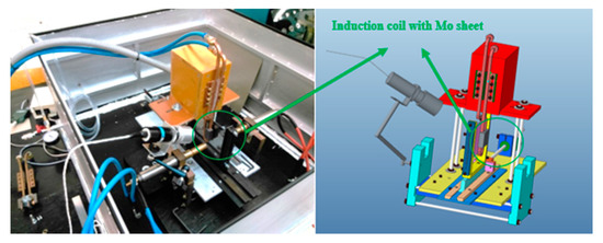
Figure 1.
Experimental set-up of induction heating of Mo sheet, Right—the 3D projection of the heating coil with Mo sheet and required assembly, Left—the physical prototype of proposed induction heating system.
- the operating frequency of the electromagnetic field
- value of the coil’s current
- distance (gap) between the heating coil and Mo sheet
Experimental measurement for the simulation model’s reference design was provided at the conditions defined by Table 1. At this point, the operating frequency is modulated with the change of the coil’s current value. The higher the current is, the value of frequency decreases.

Table 1.
Operation conditions of experimental measurement.
Figure 2 shows results from the reference measurement, and Figure 3 shows results from the simulation experiment, while the operational conditions are relevant to experimental measurement. The variable that was monitored is related to the temperature value at three different locations within the Mo sheet; so, the temperature distribution through the sheet’s surface was observed.
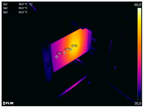
Figure 2.
Temperature distribution on the surface of Mo sheet during the experimental reference measurement.
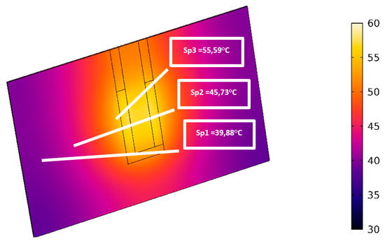
Figure 3.
Temperature distribution and its evaluation for a designed thermal simulation model of induction heating.
Table 2 evaluates the relative error between measurement and simulation at selected reference points. It is seen that the maximal error for a given situation reaches 2.52%, which presents acceptable deviation as the superior performance of simulation models is acceptable up to 5% of the relative error [17,18,19,20]. As measuring equipment, thermal infrared camera FLIR SC 640 was used, whose measuring accuracy is defined as 0.2 °C.
Table 2.
Comparisons of the temperature within reference points.
In the next sections, the design of the simulation model of induction heating of thin molybdenum sheet is presented together with the parametrical investigation of operational condition. Using the proposed model, it will be possible to investigate optimal settings related to the induction heating process.
3. Design of Electro-Thermal Simulation Model of Induction Heating
The simulation model considering induction heating of Mo sheet is designed with the use of COMSOL software. It considers a 3D model offering the options for reconfiguration of various parameters that influence the heat distribution on the Mo sheet’s surface.
These parameters are:
- the mutual position between the induction coil and the Mo sheet,
- the coil material properties as well as the coil geometry
- the frequency and intensity of the applied electromagnetic field.
The model comprises the Mo sheet, a heating coil with a magnetic core (Figure 4). The molybdenum sheet is modeled as a block (domain) with a required width (sa), depth (sb), and thickness (sc). The coil’s winding is designed as a square domain with a required thickness (ca) and the required size (cb). The coil’s core is represented by the ferrite blocks whose parameters are also reconfigurable, i.e., ferrite height (fa) and ferrite thickness (fb).
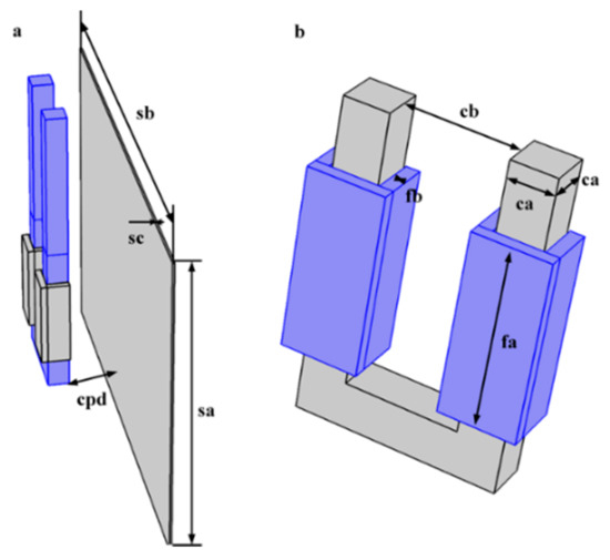
Figure 4.
The geometry descripption of the proposed induction heating model (a) and detailed geometry description of heating element - coil (b).
The variable parameter can also be the distance between the Mo sheet and heating element (cpd). The physics used in this model is “Magnetic field (MF)”. The only feature of “MF” used is “COIL”, which specifies the coil domain as a single conductor with current input surface and current output surface. All simulations are set as steady-state, frequency–domain simulations, so it is possible to determine the impact of investigated parameters on the amplitude of electromagnetic losses (heat rate) within the molybdenum sheet [4,6]. The mentioned “MF” module of the COMSOL environment uses the standard Maxwell equations for modeling an electromagnetic field in the frequency domain.
The material parameters and other model settings as final conditions settings of domains for the simulation analysis can be seen in Table 3.
Table 3.
Model settings material and final conditions.
The definitions related to the boundary conditions of the simulation model are given by domain settings (Table 4) and by equations for heat transfer/source (1)–(4). These settings are relevant for the integrated simulation software definitions related to heat transfer and electrical currents physics.
Table 4.
Boundary conditions of the induction heating model.
Equations used within the calculations are listed below:
where “ρ” is the material density, “Cp” is the specific heat capacity, “T” is the temperature, “q” is the conductive heat flux, “u” is the velocity vector, “Qe” is the external heat source, “QP” is heat created by pressure, “Qvd” is the heat source from viscous dissipation, “Qted” is the thermoelastic damping, and “k” is the thermal conductivity.
where “n” is the normal vector on the boundary, “q” is the conductive heat flux, “Q” is the heat source, and “Q0” is the actual value of the mean value of the electromagnetic losses within the domain given by electromagnetic simulation.
Because the simulation’s performance (accuracy compared to experimental results) is highly dependent on the mesh complexity and its setting, attention must be paid to the proper definition of the element size. This information for the proposed model of induction heating is listed in Table 5. The mesh for this simulation model is created as Free Tetrahedral for the whole geometry.
Table 5.
Mesh settings.
Time dependency simulation is set for 10 [s] of total time, while the time step is 0.1 [s]. The 0.1 [s] step is time, for which the results are saved, but the real computational time step is given by simulation needs (for each iteration, the convergence settings are different).
3.1. Parametric Simulation for the Determination of the Optimal Operating Conditions of the Induction Heating
For the first simulation experiment, we have focused on the parametric change of the distance between the sheet and heating element, while the induction coil geometry is unchanged. The setting for the simulation is as follows:
- The current flowing through the coil is 150 A.
- The thickness of the ferrite core is 10 mm.
- The operating frequency of the applied voltage generating EM field is 25 kHz.
- Distance (gap) between sheet and heating element is 1:1:10 [mm], i.e., initial distance is 1 mm, step is 1 mm, and the final distance is 10 mm.
In Figure 5 and Figure 6, it can be seen that the volumetric loss density, which causes heating of the molybdenum sheet, is dependent on the distance.
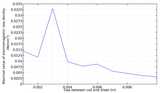
Figure 5.
The dependency of the electromagnetic losses of molybdenum sheet on the distance between the coil and the sheet.
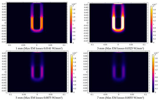
Figure 6.
Distribution of the volumetric loss density within the molybdenum sheet at different distances between heating element and sheet.
The rule that the close induction coil to the sheet is, the higher heating power will be generated is not valid because of the induction heating’s physical principles, which is influenced by the system’s operation frequency and resonance, which occurs for a given distance [21,22,23]. Figure 5 shows that the peak power is generated at the 3 mm of the gap, while below and above this value, volumetric loss decreases. For a better interpretation of the results, the distribution of these losses is shown in Figure 6.
The second simulation experiment is focused on the coil geometry’s parametric change, while the distance between the sheet and the heating element was constant (3 mm). The setting for the simulation is as follows:
- The current flowing through the coil is 150 A
- The thickness of the ferrite core is 2:1:12 mm
- The operating frequency of the applied field is 25 kHz
- Distance (gap) Between sheet and heating element is 3 mm
From Figure 7, the fluctuations of the electromagnetic loss density located at the molybdenum sheet are seen during the parametric change of the thickness of the ferrite core. This fact is related to the variations of the ferrite core’s electromagnetic excitation when its thickness is being changed. Thus, it is valid here that for the given thickness of the ferrite core and the applied field’s input parameters, a proper value of the heating element’s inductance is achieved while providing optimal magnetic path and coupling between molybdenum sheet and heating element. It ensures that the volumetric loss density within the molybdenum sheet achieves high and low values. Figure 7 shows that the peak values for volumetric loss are reached for the thickness of 4 mm and 7 mm. The result from the ferrite thickness variation is from a physical point of view, similar to the results dependent on the coil and sheet distance. For a given value of inductance, there are points with the resonance (Figure 6), which are specified by the generation of the high electromagnetic loss densities [21,22,23]. After the 7 mm thickness, the volumetric loss does not exhibit visible change.
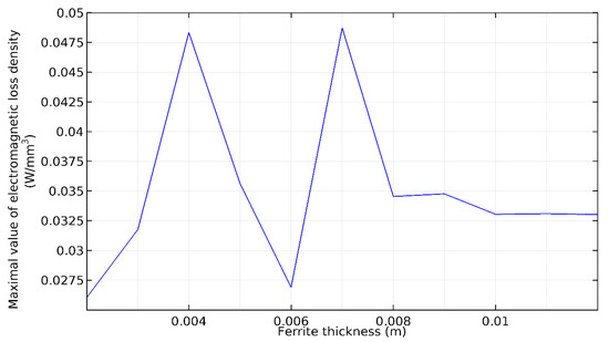
Figure 7.
The dependency of maximal electromagnetic losses within the molybdenum sheet on the ferrite thickness.
For a better interpretation of the results, the distribution of these losses is shown in Figure 8.
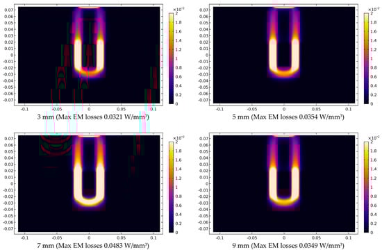
Figure 8.
Distribution of the volumetric loss density within the molybdenum sheet at different geometry of the ferrite thickness.
The last parametric evaluation focuses on investigating the impact of the value of the applied electromagnetic field (Figure 9).
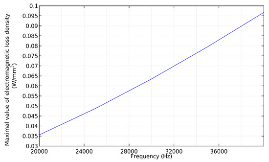
Figure 9.
The dependency of maximal electromagnetic volumetric losses within the molybdenum sheet on the operating frequency.
These relationships have been investigated for the constant distance between the heating element and sheet and for the ferrite’s constant geometry. The values were selected based on previous results, whereby the solution with the highest volumetric loss on the sheet was selected. The settings for these types of simulations are as follows:
- The current flowing through the coil is 150 A.
- The thickness of the ferrite core is 7 mm.
- The applied field’s operating frequency is 20:5:40 kHz (initial frequency 20 kHz, step-change 5 kHz, and final frequency 40 kHz).
- Distance (gap) between sheet and heating element is 3 mm.
Figure 10 shows that with the increase of the EM field’s operating frequency, the volumetric losses within the molybdenum sheet increase almost linearly. The experiment was realized for the range from 20 kHz up to 40 kHz. Within this range, the saturation of ferrite material is avoided. The optimal operation point for this experiment was reached at 40 kHz. Above this value, the magnetic saturation will cause a decrease in the value of inductance; thus, the coupling shall also be disturbed, and the required heat rate within the molybdenum sheet shall be insufficient.
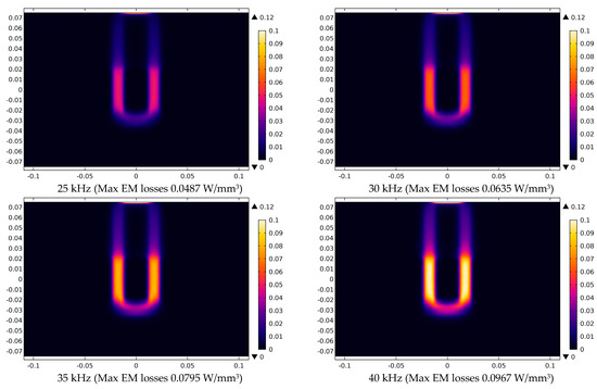
Figure 10.
Distribution of the volumetric loss density within the molybdenum sheet at selected values of the operating frequency.
3.2. Heat Distribution and Heat Performance for Optimal Parameter Settings of Induction Heating
The simulation experiments previously realized uses results to determine the dependency between the parameters settings and volumetric power losses within the molybdenum. Those optimal settings have been adapted here, and the only change during parametric simulation will be the value of the coil’s current.
- The current flowing through the coil is 50:50:500 A.
- The thickness of the ferrite core is 7 mm.
- The operating frequency of the applied field is 40 kHz.
- Distance (gap) between sheet and heating element is 3 mm.
Figure 11 and Figure 12 show that with the increase of the coil’s current, the sheet’s volumetric losses and the generated power of the coil rises. The limitation within this experiment was given on the current value, which cannot exceed 500 A due to the electrical parameters of the heating element’s conductor.
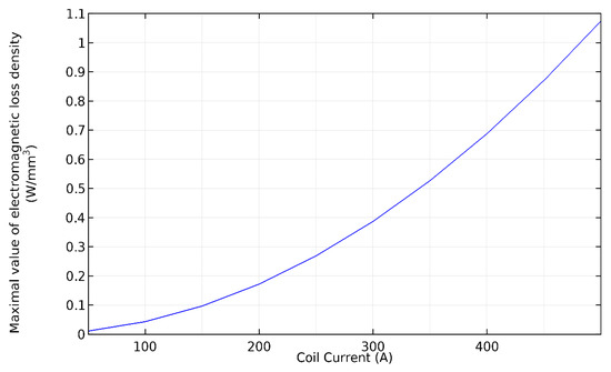
Figure 11.
The dependency of maximal electromagnetic losses within the molybdenum sheet on the value of the coil’s current.
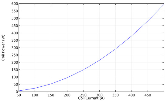
Figure 12.
The dependency of coil power on the value of the coil’s current.
This behavior is based on the basic laws of the accumulation of energy within the inductor. Figure 11 shows that the energy has exponential character; thus, it is confirmed here that energy is proportional to the value of inductance and square of the current flowing through the inductor.
Figure 13 shows the distribution of the volumetric losses within the molybdenum sheet for selected values of the coil’s current. The purpose of this research was to identify the amount of volumetric loss. Simultaneously, these values will consequently serve within the thermal simulation of the induction heating, where the input boundary condition for the heating is identified values of molybdenum sheet losses.
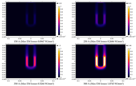
Figure 13.
Distribution of the volumetric loss density within the molybdenum sheet at different values of the coil’s current.
Simultaneously, the temperature distribution within the Mo sheet’s surface was recorded during the time-dependent simulation (Figure 14). Figure 14 is showing the temperature distribution for the parameter settings from Table 4, Table 5 and Table 6. The simulation has time-dependency; thus, the first result is valid for 10 s of the heating process, while the second is valid for 130 s of the heating process. It is seen that the maximum temperature is located around the heating element and reaches 650 °C.
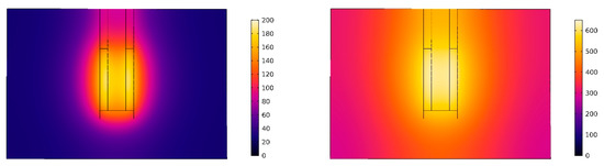
Figure 14.
Temperature distribution for optimal setting of induction heating parameters during time-dependent simulation, after 10 s (left), and after 130 s (right).
Table 6.
Optimal operational parameters settings.
After getting relevant information for the optimal operational parameters setting, the experiment defined by all optimal measures was realized. Figure 15 represents the situation as mentioned above, while it is seen that the temperature distribution refers to the results achieved during the simulation result (Figure 14—right). There is a slight difference at the maximum temperature achieved at the Mo sheet hotspot (626 °C) instead of the simulation (607 °C). Even there is a difference, it is evident that the research of the optimal parameter settings of the induction heating through a simulation approach gives satisfying results. The model shall serve for any optimization purposes needed for the induction heating.
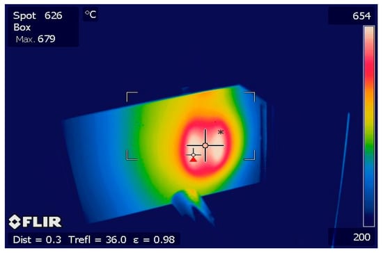
Figure 15.
Experimental measurement for the optimal settings of parameters of induction heating of Mo sheet.
Experimental results of the induction heating supported by the optimal settings received from simulations have been compared to the different heating processes, i.e., contact resistive heating (Figure 16). This comparison demonstrates that induction heating provides a more uniform temperature distribution than alternative heating techniques [24,25,26]. The maximal difference (diffT) between the area with the lowest and the highest temperature for induction heating is lower than resistive heating (diffTind = 150 °C, diffTres = 225 °C). Based on the obtained results, it is expected that with consequent utilization of the translation move during optimal induction heating setting, the thermal distribution within Mo sheet will satisfy the required forming performance.
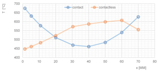
Figure 16.
Comparison of the temperature distribution in the direction of the cut at the surface of the investigated molybdenum plate considering contact heating and induction heating.
4. Conclusions
The presented paper discusses the possibilities of the heating of molybdenum sheets required for the forming purposes when the sapphire’s crystallization is considered. For those activities, the most important issue is related to the heating system design, whose ability will facilitate uniform heat distribution and required temperature values within the molybdenum sheet’s surface/volume. The paper presents several approaches to reaching required properties, mostly based on detailed modeling of the induction heating method [27,28]. Initially, the designed model was compared to the reference measurement. Consequently, the investigation procedure of inductive heating’s operational conditions was realized to identify optimal operational parameters. At the end of the paper, the results from the simulation with optimal settings are shown. The experiment was set based on the simulation results, which define the induction heating’s optimal setting. Comparison between simulation and measurement showed a very close similarity of heat distribution within the Mo sheet surface. The main difference is visible if hotspots are observed. The measurement exhibits 20 °C higher temperature compared to simulation. The reasons for this difference can be several. The main contribution to this discrepancy is the non-linear temperature dependence of the thermophysical characteristics of air and materials located within the proposed system and consequent sensitivity settings of the simulation parameters (simulation steps, mesh size). These errors can be improved by finer simulation settings or by integrating the parameter fittings function of the material’s thermal dependencies [29,30]. Based on the achieved results, it can be said that proposed modeling gives satisfying results and gives opportunities for optimization procedures for various types of Mo sheets’ heating processes.
Author Contributions
Conceptualization and writing—original, M.F.; investigation and draft preparation, M.P.; methodology, resources, T.D. All authors have read and agreed to the published version of the manuscript.
Funding
This research received no external funding.
Institutional Review Board Statement
Not applicable.
Informed Consent Statement
Not applicable.
Data Availability Statement
Not applicable.
Acknowledgments
This publication was realized with the support of Operational Program Integrated Infrastructure 2014–2020 of the project: Innovative Solutions for Propulsion, Power and Safety Components of Transport Vehicles, code ITMS 313011V334, cofinanced by the European Regional Development Fund.
Conflicts of Interest
The authors declare no conflict of interest.
References
- Pepper, I.; Gerba, C.; Gentry, T. Enviromental Microbiology, 3rd ed.; Elsevier: Amsterdam, The Netherlands, 2013. [Google Scholar]
- Griffiths, A.; Miller, J.; Suzuki, D. An Introduction to Genetic Analysis, 7th ed.; W.H. Freeman: New York, NY, USA, 2000. [Google Scholar]
- Fasihi, Z.; Zakeri-Milani, P.; Nokhodchi, A.; Akbari, J.; Barzegar-Jalali, M.; Loebenberg, R.; Valizadeh, H. Thermodynamic approaches for the prediction of oral drug absorption. J. Therm. Anal. Calorim. 2017, 130, 1371–1382. [Google Scholar] [CrossRef]
- Guihong, T.M.; Christopher, F.; Change, T. Temperature-Sensitive Mutations Made Easy: Generating Conditional Mutations by Using Temperature-Sensitive Inteins That Function within Different Temperature. Genetics 2009, 183, 13–22. [Google Scholar]
- Koniar, D.; Hargas, L.; Stofan, S. High Speed Video System for Tissue Measurement Based on PWM Regulated Dimming and Virtual Instrumentation. Elektron. Elektrotech. 2010, 10, 169–172. [Google Scholar]
- Kuo-Chi, L. Thermal propagation analysis for living tissue with surface heating. Int. J. Ther. Sci. 2008, 47, 507–513. [Google Scholar]
- Verma, R. Challenges in education in thermal analysis and calorimetry. J. Therm. Anal. Calorim. 2013, 113, 1675–1679. [Google Scholar] [CrossRef]
- Agrawal, M.; Pardasani, K.R.; Adlakha, N. Finite element model to study the thermal effect of tumors in dermal regions of irregular tapered shaped human limbs. Int. J. Ther. Sci. 2015, 98, 287–295. [Google Scholar] [CrossRef]
- Su, C.-H.; Wu, S.-H.; Shen, S.-J.; Shiue, G.-Y.; Wang, Y.-W.; Shu, C.-M. Thermal characteristics and regeneration analyses of adsorbents by differential scanning calorimetry and scanning electron microscope. J. Therm. Anal. Calorim. 2009, 96, 765–769. [Google Scholar] [CrossRef]
- Kéri, O.; Bárdos, P.; Boyadjiev, S.; Igricz, T.; Nagy, Z.K.; Szilágyi, I.M. Thermal properties of electrospun polyvinylpyrrolidone/titanium tetraisopropoxide composite nanofibers. J. Therm. Anal. Calorim. 2019, 137, 1249–1254. [Google Scholar] [CrossRef]
- Shunmugam, M.S.; Kanthababu, M. Advances in Simulation, Product Design and Development. In Advances in Simulation, Product Design and Development, Proceedings of the AIMTDR 2018, Berlin/Heidelberg, Germany, 6 November 2018; Springer: Berlin/Heidelberg, Germany, 2018; ISBN 978-981-329-487-5. [Google Scholar]
- Veeman, D. Finite Element simulation of Temperature Distribution and Residual Stress in Single Bead on Plate Weld Trial using Double Ellipsoidal Heat Source Model. Int. J. Recent Technol. Eng. 2019, 8, 133–138. [Google Scholar]
- Hyoe, T.; Colegrove, P.A.; Shercliff, H. Thermal and microstructure modelling in thick plate aluminium alloy 7075 friction stir welds. In Friction Stir Welding and Processing II, Proceedings of the 2nd International Conference on Friction Stir Welding and Processing, San Diego, CA, USA, 13–16 September 2003; The Minerals, Metals and Materials Society: Pittsburgh, PA, USA, 2003; pp. 33–42. [Google Scholar]
- Ubaid, M.; Bajaj, D.; Mukhopadhyay, A.K.; Siddiquee, A.N. Friction Stir Welding of Thick AA2519 Alloy: Defect Elimination, Mechanical and Micro-Structural Characterization. Met. Mater. Int. 2019, 26, 1841–1860. [Google Scholar] [CrossRef]
- Yuan, W.-J.; Wu, Y.-X. Coupled thermal-mechanical simulation on quenching of aluminum alloy thick-plate based on ANSYS. J. Cent. South Univ. Sci. Technol. 2010, 41, 2207–2212. [Google Scholar]
- Colegrove, P.; Shercliff, H.R. CFD modelling of friction stir welding of thick plate 7449 aluminium alloy. Sci. Technol. Weld. Join. 2006, 11, 429–441. [Google Scholar] [CrossRef]
- Hargas, L.; Koniar, D.; Hrianka, M. Adjusting and Conditioning of High Speed Videosequences for Diagnostic Purposes in Medicine. In Proceedings of the 10th International Conference ELEKTRO 2014, Rajecké Teplice, Slovakia, 19–20 May 2014; pp. 548–552. [Google Scholar]
- Nomoto, T.; Imajo, S.; Yamashita, S.; Akutsu, H.; Nakazawa, Y.; Krivchikov, A.I. Construction of a thermal conductivity measurement system for small single crystals of organic conductors. J. Therm. Anal. Calorim. 2018, 135, 2831–2836. [Google Scholar] [CrossRef]
- Ge, M.Y.; Shu, C.; Chua, K.J.; Yang, W.M. Numerical analysis of a clinically-extracted vascular tissue during cryo-freezing using immersed boundary method. Int. J. Ther. Sci. 2016, 110, 109–118. [Google Scholar] [CrossRef]
- Chen, M.; Dongxu, O.; Cao, S.; Liu, J.; Wang, Z.; Wang, J. Effects of heat treatment and SOC on fire behaviors of lithium-ion batteries pack. J. Therm. Anal. Calorim. 2018, 136, 2429–2437. [Google Scholar] [CrossRef]
- Hruska, K.; Kindl, V.; Pechanek, R. Design and FEM Analyses of an Electrically Excited Automotive Synchronous Motor. In Proceedings of the 15th International Power Electronics and Motion Control Conference and Exposition (EPE-PEMC ECCE Europe), Novi Sad, Serbia, 4–6 September 2012. [Google Scholar]
- Rafajdus, P.; Peniak, A.; Peter, D.; Makyś, P.; Szabó, L. Optimization of Switched Reluctance Motor Design Procedure for Electrical Vehicles. In Proceedings of the International Conference on Optimization of Electrical and Electronic Equipment (OPTIM), Brasov, Romania, 22–24 May 2014. [Google Scholar]
- Koniar, D.; Hargas, L.; Loncova, Z. Visual system-based object tracking using image segmentation for biomedical applications. Electr. Eng. 2017, 99, 1349–1366. [Google Scholar] [CrossRef]
- Frivaldsky, M.; Donic, T.; Vavrus, V.; Pavelek, M. Experimental research of optimization methodology for local, resistive—Heating of thin molybdenum plates. Int. J. Ther. Sci. 2017, 121, 111–123. [Google Scholar] [CrossRef]
- Zhu, J.; Fu, S.; Li, K.; Zeng, X.; Chen, S. Thermal stability assessment of a new energetic Ca(II) compound with ZTO ligand by DSC and ARC. J. Therm. Anal. Calorim. 2018, 134, 1873–1882. [Google Scholar] [CrossRef]
- Mashayekhi, R.; Khodabandeh, E.; Akbari, O.A.; Toghraie, D.; Bahiraei, M.; Gholami, M. CFD analysis of thermal and hydrodynamic characteristics of hybrid nanofluid in a new designed sinusoidal double-layered microchannel heat sink. J. Therm. Anal. Calorim. 2018, 134, 2305–2315. [Google Scholar] [CrossRef]
- Hațiegan, C.; Răduca, M.; Frunzaverde, D.; Răduca, E.; Pop, N.; Gillich, G.-R. The modeling and simulation of the thermal analysis on the hydrogenerator stator winding insulation. J. Therm. Anal. Calorim. 2013, 113, 1217–1221. [Google Scholar] [CrossRef]
- Balek, V.; Zelenák, V.; Mitsuhashi, T.; Beckman, I.N.; Haneda, H.; Bezdička, P. Thermal Behaviour of Titania Based Materials: Mathematical modeling of emanation thermal analysis results. J. Therm. Anal. Calorim. 2002, 67, 63–72. [Google Scholar] [CrossRef]
- Barewar, S.D.; Tawri, S.; Chougule, S.S. Experimental investigation of thermal conductivity and its ANN modeling for glycol-based Ag/ZnO hybrid nanofluids with low concentration. J. Therm. Anal. Calorim. 2019, 139, 1779–1790. [Google Scholar] [CrossRef]
- Kozlov, A.; Svishchev, D.; Donskoy, I.; Keiko, A.V. Thermal analysis in numerical thermodynamic modeling of solid fuel conversion. J. Therm. Anal. Calorim. 2012, 109, 1311–1317. [Google Scholar] [CrossRef]


Publisher’s Note: MDPI stays neutral with regard to jurisdictional claims in published maps and institutional affiliations. |
© 2021 by the authors. Licensee MDPI, Basel, Switzerland. This article is an open access article distributed under the terms and conditions of the Creative Commons Attribution (CC BY) license (http://creativecommons.org/licenses/by/4.0/).