Multi-Model Identification of HVAC System

Abstract

Heat, ventilation and air conditioning (HVAC) is a crucial system for maintaining acceptable air quality and keeping the building and its occupants healthy. There are some challenges in controlling and identifying this system as it commonly operates in different operation conditions. Furthermore, various types of un-controlled sources disturb the steady operations. In addition, an HVAC system is an inherently nonlinear system and varies with time. As a result, conventional methods are not successful in identifying and controlling this system. This paper proposes a new multi-model approach in which the clustering and regression steps are performed simultaneously to tackle this problem. Cost functions of clustering and regression steps are combined and optimized using an iterative algorithm. After identifying the local models, a gap metric based approach is used to develop a global model of the process. The proposed approach is tested on a simulated ventilation unit system and real-world dataset. The results show the performance of the proposed method of identifying the ventilation system.

1. Introduction

Nowadays, heat, ventilation, and air conditioning (HVAC) systems are essential for indoor air quality, thereby on occupants’ health and comfortability. Due to nonlinearity and uncertainty, it is inaccurate to identify this process using conventional and first-principle models. Hence, during the last decade, many papers have been published on identifying this system using data-driven methods [1,2,3,4]. However, these data are commonly sampled from one operation region, so they are not general enough to predict the system behavior in other operating conditions. Although varying operation condition is common in an HVAC system, traditional identification approaches are usually calculated for a single operating mode—under stationary conditions. One possible solution is to utilize a multi-model approach to deal with the problem of multi-mode and nonlinear process operations.

The multi-model approach’s main idea is to represent the nonlinear system with a combination of (weighted) linear models. The main challenges of this approach are determining the sufficient number of models, local model weights, as well as the operation points in which the linear models should be constructed. These challenges are more cumbersome when no information about the system operation is available, so the operation point and clustering should be done just by using routine operating data.

One possible approach is to separate nonstationary data into several stationary ones to overcome the problem of multi-model operations. In this way, each stationary operation mode can be interpreted as a single steady-state operation. Then, the linear approach can be conducted for each stationary portion of data. This task requires executing clustering and identification, each of which has its cost function. Implementing these two tasks separately cannot guarantee global optimality. For instance, let us assume that we have obtained an optimal solution for clustering data into different operating modes. That optimal solution might not lead to an optimal solution for the identification of models. A hybrid approach is required to incorporate individual cost functions of dynamic clustering and model identification to form a single cost function to resolve this problem. This can be accomplished using a support vectors-based identification method, which is introduced in this paper. To identify models for each labeled group of data (cluster), support vector (SV) regression is applied, aiming to maximize the distance between models and decrease the mean square of the overall residuals.

As mentioned, optimality in individual steps of clustering and regression does not necessarily lead to overall optimality, which is due to their different objectives. This paper aims to align the goals of these two steps to predict variables. To this end, the SV method is extended to handling clustering and regression analysis simultaneously. In this way, we are able to ensure the optimality of prediction.

After deciding and identifying the local linear models, the question is how to construct the global model using the local linear models. One possible way to build a global model is assigning weights to each local model. The weights are commonly calculated using distances between local models.

In [5], Galan et al. suggested using the gap metric, which measures the distance between two linear models, as a guideline for selecting local models. The distance should not be larger than a prescribed threshold level. The advantage of the method is no detailed information about the nonlinear model of the system is required. Furthermore, by this approach, the number of local models can also be determined. To decide the operation point for the construction of local models, the measure of nonlinearity approach [6,7] can be utilized. The idea behind this approach is constructing the local linear models on operating points near which the system is most nonlinear to cover the nonlinearity of the system. The disadvantage of this method is the complication in computing the nonlinearity measure.

After deciding each local model, the global model can be determined by combining the local models using either so-called hard or soft switching approaches. In the hard switching approach, the best possible local model is selected and analyzed. In the soft switching approach, the global model is formed by a weighted sum of the local models.

There are many weighting functions, such as gap metric based weighting [8], Bayesian weighting functions [9], and trapezoidal functions [10]. The gap metric-based weighting method has been extensively used; see [11,12,13].

The advantages of using a weighted gap in the multi-model approach include (1) the performance can be incorporated in selecting operating points, and (2) soft switching, which avoids high-frequency switching.

The proposed method of identifying local models uses simultaneous clustering and regression, then a global model using a weighted sum of local models is tested on a simulated HVAC system. In this test, the simulated building has three zones. The proposed method is used to identify the behavior of the ventilation system in stabilizing the zones’ temperature, while there are different sources of disturbances and outdoor temperature changes in a range of −25 °C to 25 °C. The proposed method is also tested on a real-world dataset. The results show that the proposed method is capable of identifying that the operating conditions of the nonlinear HVAC system are changing due to disturbances.

The remainder of the paper is organized as follows: In Section 2, the proposed simultaneous clustering and regression method is presented. In Section 3, the global model is built using the gap metric method. Section 4 presents the identified models based on datasets obtained from a simulated ventilation system and real-world dataset using the proposed multi-model framework. In Section 5, concluding remarks are drawn.

2. The Proposed Simultaneous Clustering and Regression Method

Ben-Hur et al. [14] proposed a clustering method that utilizes a support vector (SV) to define a cost function. In this work, we use the support vector-based clustering (SVC) proposed by [14], and make modifications in order to make it compatible with our framework. Recall the input space as X ∈ R^N×M.

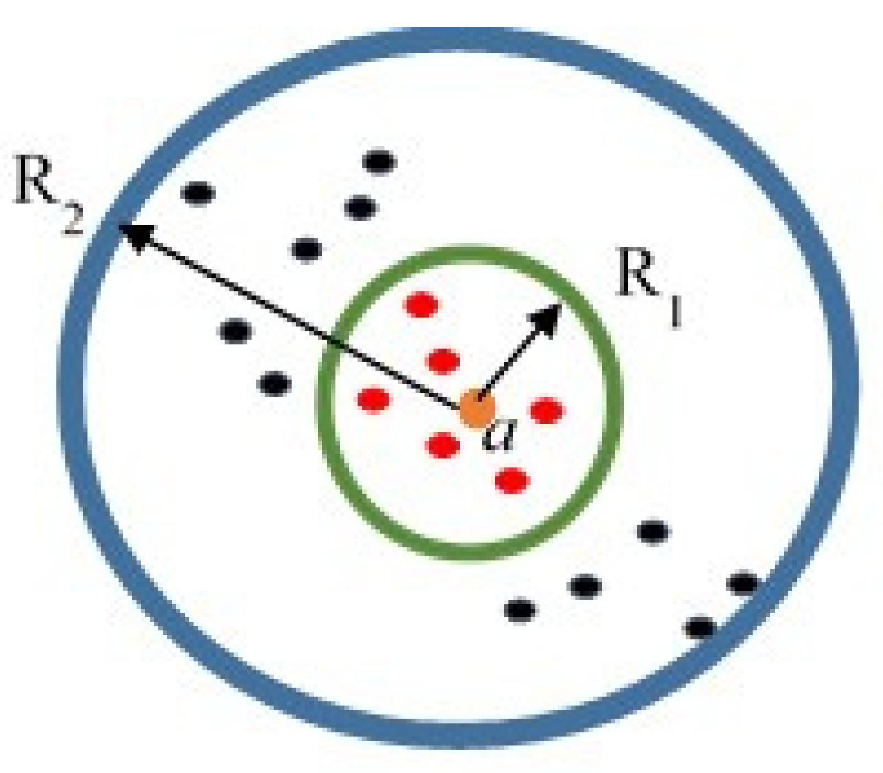
In this method, any point that has a smaller distance than R₁ from point a (center of all circles) is classified in cluster 1 (red dots in Figure 1), and the same for cluster 2 (black dots in Figure 1). To find the center (a) and each R_i, one needs to solve an optimization problem:

$$\begin{gathered} mi{n}_{a.R_i^2} R_i^2 \\ \mathrm{Subject} \mathrm{to}: ||x_k-{a\left|\right|}^2\le R_i^2. i=\left\{1.2.\cdots .h\right\} \end{gathered}$$

(1)

where h denotes the number of clusters and || • || represents the Euclidean distance. By solving the above-mentioned objective function, the boundaries of the clusters can be obtained.

Considering that the data may not be separable by spherical shape clusters, we modify this approach. In the modified approach, the centers of clusters are not fixed points. Instead, the center of the clusters come from the dynamic models. To assign each point to a cluster, the distances between the point and all dynamic models (i.e., the model error or residual) are used. The point will be assigned to the cluster in which the the associated dynamic model produces the lowest residual error. In other words, among all dynamic models, the point belongs to the dynamic model with the lowest local error, and thus the point is assigned to that mode (cluster).

Suppose that data are gathered from a general model switching between h linear models I_i, i = 1, …,h, defined as

$$y_k=\langle w_i. x_k\rangle . if x_k\in I_i$$

(2)

where w_i contains the parameters of the linear model and x_k is the corresponding repressors, and <•> denotes inner product operation. In this paper, the ARX model (where $x_k={\left[y_{k-1}. y_{k-2.}\cdots .y_{k-n_y}.u_k.u_{k-1}.\cdots .u_{k-n_u}\right]}^T$ and $w_i=\left[a_1^i.a_2^i.\cdots .a_{n_y}^i.b_1^i.b_2^i.\cdots .b_{n_u}^i\right]$) is used for HVAC system identification. In this model, $y_k$ and $u_k$ are system outputs and inputs, respectively; $n_y$ and $n_u$ denote orders of system outputs and inputs in the model, and $a_j^i$ and $b_k^i$ for $j=1.\cdots .n_y$ and $k=1.\cdots .n_u$ are model parameters associated with outputs and inputs terms, respectively.

Obviously, if the point (x_k, y_k) is generated by model i, then its distance from that model will be the smallest compared to others. So, an intuitive way to determine a cluster for the point (x_k, y_k), is calculating the distances of the point from each of the models and assigning it to the cluster in which the corresponding model generates the lowest error. This way, the dynamic models are regarded as the centers, and the corresponding errors are used to determine the clusters.

As mentioned, the cluster center in [14] is supposed to be known, but this is not the case in our application. Therefore, it is required to perform identification along with clustering. In order to aggregate clustering and regression steps, we propose the following cost function in which the first term corresponds to clustering and the second to regression. The regression cost function is inspired by the epsilon-support vector regression method.

$$\begin{gathered} mi{n}_{R_i.z_{k.i}. w_i} v\left[{\displaystyle \sum }_{i=1}^h{R}_i^2+C{\displaystyle \sum }_{k=1}^N{\displaystyle \sum }_{i=1}^h{z}_{k.i}{}^m{r}_{k.i}{}^2\right]+\frac{\mu }{2}\left[{\displaystyle \sum }_{i=1}^h||w_i||{}^2\right] \\ \mathrm{Subject} \mathrm{to}: \{\begin{array}{c}{y}_k-⟨w_i.x_k⟩\le \epsilon \\ ⟨w_i.x_k⟩-y_k\le \epsilon \\ \end{array} if \left(x_k.y_k\right) \in I_i \\ {z}_{k.i}{}^m{r}_{k.i}{}^2\le R_i^2. if \left(x_k.y_k\right) \in I_i and i=\left\{1.2.\cdots .h\right\} \\ {\displaystyle \sum }_{i=1}^h{z}_{k.i}=1 \\ 0\le z_{k.i}\le 1 \end{gathered}$$

(3)

where µ and ν are weighting coefficients, m > 1 is a weighting exponent on each membership $z_{k.i}$, $r_{k.i}=y_k-w_i.x_k$ denotes the model regression error for each mode i, and $z_{k.i}$ determines the probability of point (x_k,y_k) belongs to cluster i (model i). Therefore, each point has an association with all models but with different probabilities. In addition, R_i determines the boundary of the cluster i. By supposing the point belongs to cluster i (x_k,y_k) (i.e., $z_{k.i}=1$), in the residual space, R_i can be interpreted as the cluster radius as $\left|\right|r_i\left|\right|{}^2\le R_i^2$. Given the system models (cluster centers), minimizing the cost function provides the optimal cluster boundary.

The key idea to solving the optimization problem (3) is to construct a Lagrange function from the objective function (3), which means that the gradient of its Lagrangian (4) with respect to the primal variables $\left(R_i.w_i.r_{k.i}.z_{k.i}\right)$ must vanish.

$$\begin{array}{cc}\hfill L=v{\displaystyle {\displaystyle \sum }_{i=1}^h}{R}_i^2+& \frac{\mu }{2}{\displaystyle {\displaystyle \sum }_{i=1}^h}||w_i||{}^2+\frac{\rho }{2}{\displaystyle {\displaystyle \sum }_{k=1}^N}{\displaystyle {\displaystyle \sum }_{i=1}^h}{z}_{k.i}{}^m{r}_{k.i}{}^2\hfill \\ & -{\displaystyle {\displaystyle \sum }_{k=1}^N}{\displaystyle {\displaystyle \sum }_{i=1}^h}{\alpha }_{k.i}{z}_{k.i}{}^m\left\{r_{k.i}-\left(y_k-⟨w_i.x_k⟩\right)\right\}\hfill \\ & -{\displaystyle {\displaystyle \sum }_{k=1}^N}{\displaystyle {\displaystyle \sum }_{i=1}^h}{\sigma }_{k.i}\left\{R_i-z_{k.i}{}^m{r}_{k.i}{}^2\right\}-\gamma \left({\displaystyle {\displaystyle \sum }_{i=1}^h}{z}_{k.i}-1\right)\hfill \end{array}$$

(4)

where ${\sigma }_{k.i}$ and ${\alpha }_{k.i}$ are Lagrange multipliers.

The conditions for optimality are given by

$$\begin{gathered} \frac{\partial L}{\partial z_{k.i}}=m{z}_{k.i}{}^{m-1}\left({\sigma }_{k.i}+\frac{\rho }{2}\right)r_{k.i}{}^2-\gamma -m{z}_{k.i}{}^{m-1}{\sigma }_{k.i}\left\{r_{k.i}-\left(y_k-⟨w_i.x_k⟩\right)\right\}=0 \\ \frac{\partial L}{\partial w_i}=\mu w_i-{\displaystyle \sum }_{k=1}^N{\alpha }_{k.i}{z}_{k.i}{}^m{x}_k=0 \\ \frac{\partial L}{\partial r_{k.i}}=z_{k.i}{}^m\left(\rho r_{k.i}-{\alpha }_{k.i}+2{\sigma }_{k.i}{r}_{k.i}\right)=0 \\ \frac{\partial L}{\partial R_i}=2v{R}_i-{\displaystyle \sum }_{k=1}^N{\sigma }_{k.i}=0 \\ \frac{\partial L}{\partial {\alpha }_{k.i}}=z_{k.i}{}^m\left\{r_{k.i}-\left(y_k-⟨w_i.x_k⟩\right)\right\}=0 \\ \frac{\partial L}{\partial {\sigma }_{k.i}}=R_i-z_{k.i}{}^m{r}_{k.i}{}^2=0 \\ \frac{\partial L}{\partial \gamma }={\displaystyle \sum }_{i=1}^h{z}_{k.i}-1=0 \\ {\sigma }_{k.i}\left\{R_i-z_{k.i}{}^m{r}_{k.i}{}^2\right\}=0 \\ {R}_i\ge z_{k.i}{}^m\left|\right|y_k-⟨w_i.x_k⟩\left|\right|{}^2=z_{k.i}{}^m{r}_{k.i}{}^2 \end{gathered}$$

(5)

The partial derivatives of L with respect to the primal variables $\left(R_i.w_i.r_{k.i}.z_{k.i}\right)$ should be equal to zero for optimality. By doing some simple calculation, we reach to the following solution:

$$\begin{gathered} z_{k.i}=\raisebox{1ex}{$1$}\!\left/ \!\raisebox{-1ex}{${{\displaystyle \sum }}_{s=1}^h{\left(\frac{r_{k.i}}{r_{k.s}}\right)}^{\frac{2m}{m-1}}$}\right. \\ {w}_i=\frac{1}{\mu }{\displaystyle \sum }_{k=1}^N{\alpha }_{k.i}{z}_{k.i}{}^m{x}_k \\ {R}_i=\frac{1}{2v}{\displaystyle \sum }_{k=1}^N{\sigma }_{k.i} \\ {r}_{k.i}=\frac{{\alpha }_{k.i}}{\left(\rho +2{\sigma }_{k.i}\right)} \end{gathered}$$

(6)

The Algorithm 1 gives instruction to develop a multi-mode model given the input and output data of the system.

Algorithm 1

Step 1—Select proper values for m, h and construct regressor and observation vector $\left(x_k.y_k\right)$. Step 2—Initialize the probability vector $z_{k.i}$ for each cluster i by a random number generator. Step 3—Iterate the algorithm until $z_{k.i}$ converges or termination criterion is satisfied. Step 4—Update residual values $r_{k.i}$ for each cluster i. Step 5—Update parameters ${\sigma }_{k.i}$, $R_i$ and $w_i$. Step 6—Update $z_{k.i}$ as $z_{k.i}=\raisebox{1ex}{$1$}\!\left/ \!\raisebox{-1ex}{${{\displaystyle \sum }}_{s=1}^h{\left(\frac{r_{k.i}}{r_{k.s}}\right)}^{\frac{2m}{m-1}}$}\right.$ Step 7—Go to step 3, and repeat until convergence.

3. Gap Metric

Distance between any two given plant models P₁ and P₂, can be defined by a gap metric. Let P_i, i = 1, 2 be p × m rational transfer function matrices, and $P_i=N_i{M}_i^{-1}={\tilde{M}}_i^{-1}{\tilde{N}}_i,\hspace{1em}i=1,2$ denote the normalized right/left coprime factorizations of P₁ and P₂, respectively. In the gap metric, the distance between the two plants P₁ and P₂ in the frequency domain is defined as:

$$\kappa \left(P_1,P_2\right)\left(\omega \right)=\overline{\sigma }\left({\tilde{N}}_2{M}_1-{\tilde{M}}_2{N}_1\right)\left(\omega \right)$$

(7)

where $\overline{\sigma }\left(A\right)\left(\omega \right)$ stands for the maximum singular value of A at frequency w. It is known that $\kappa \left(P_1,P_2\right)\left(\omega \right)\le 1\hspace{1em}\forall \omega$ [13]. With the distance function (7), the gap metric is defined as

$$\delta \left(P_1,P_2\right)=\{\begin{array}{c}\begin{array}{l}\underset{\omega }{\sup }\hspace{1em}\kappa \left(P_1,P_2\right)\left(\omega \right)\hspace{1em}\hspace{1em}if\hspace{0.17em}\det \left(M_1^{*}{M}_2+N_1^{*}{N}_2\right)\ne 0\hspace{1em}\forall \omega \\ \hspace{1em}\hspace{1em}\hspace{1em}\hspace{1em}\hspace{1em}\hspace{1em}\hspace{1em}\hspace{1em}\hspace{1em}\hspace{1em}and\hspace{0.17em}wno\det \left(M_1^{*}{M}_2+N_1^{*}{N}_2\right)=0,\end{array}\\ 1\hspace{1em}\hspace{1em}\hspace{1em}\hspace{1em}\hspace{1em}\hspace{1em}\hspace{1em}\hspace{1em}\hspace{1em}\hspace{1em}\hspace{1em}\hspace{1em}\hspace{1em}\hspace{1em}\hspace{1em}\hspace{1em}\hspace{1em}\hspace{1em}otherwise.\end{array}$$

(8)

where det(A) stands for the determinant of the matrix A, $M^{*}\left(s\right)=M^T\left(-s\right)$ stands for the conjugate transpose of any $M\left(s\right)$, and wno(f(s)) stands for the winding number about the origin of the scalar function f(s) as s follows the standard Nyquist D-contour [13]. The defined gap metric has the following properties:

(1)

$0\le \delta \left(P_1,P_2\right)\le 1$.

(2)

The gap metric is an extension of common distance measures between two linear systems such as the infinity norm. For instance, the distances between two systems $P_1=\raisebox{1ex}{$1$}\!\left/ \!\raisebox{-1ex}{$s$}\right.$ and $P_2=\raisebox{1ex}{$1$}\!\left/ \!\raisebox{-1ex}{$s+0.1$}\right.$ in the sense of infinity norm and gap metric are infinity and 0.1, respectively.

(3)

One pro of the gap metric is that it measures the ‘distance’ in the closed-loop sense instead of the open-loop sense. In other words, a small distance between two systems in the gap metric sense means that there exists at least one feedback controller that stabilizes both systems and the distance between the closed loops is small in the infinity norm sense. For instance, for the distance between two systems $P_1=\raisebox{1ex}{$100$}\!\left/ \!\raisebox{-1ex}{$2s+1$}\right.$ and $P_2=\raisebox{1ex}{$100$}\!\left/ \!\raisebox{-1ex}{$2s-1$}\right.$ the gap metric is about 0.2 [13].

3.1. Proper Number of Mode Selection

It is possible that some of the identified local models using the proposed method in the previous section are similar, i.e., the gap metric distance between these models is neglectable. Hence, the Gap metric is employed to merge the linear models that are similar. Using this strategy, a plentiful number of local models can be constructed.

The algorithm for constructing local models is as follows:

(1)

Initialize the operation regions and calculate the nonlinear measure index for each operating region. Select enough operation points in each operating region.

(2)

Collect enough data from the system around the operating point OPi, use the proposed Algorithm 1 and get the linear models Pi.

(3)

Compute the gap metric between all pairs of linear models P_i and P_j (i.e., $\delta \left(P_i,P_j\right)\hspace{1em}i,j=1,\dots ,N$).

(4)

Prescribe a threshold level τ. Cluster the local models that satisfy δj ≤ τ.

3.2. Local Model Weights

To determine the weights for each local model, the gap metric can be utilized. To this end, assume there exist N local models (P_i, i = 1, …, N). The weights are updated at a discrete time interval (i). We assign the weights for each local model using the following formula

$$w_i=\frac{1-{\delta }_i}{{{\displaystyle \sum }}_{i=1}^N\left(1-{\delta }_i\right)}$$

(9)

where ${\delta }_i$ is the gap metric between each local model i and current model at time instance i.

4. Simulation and Validation

4.1. Simulation Results

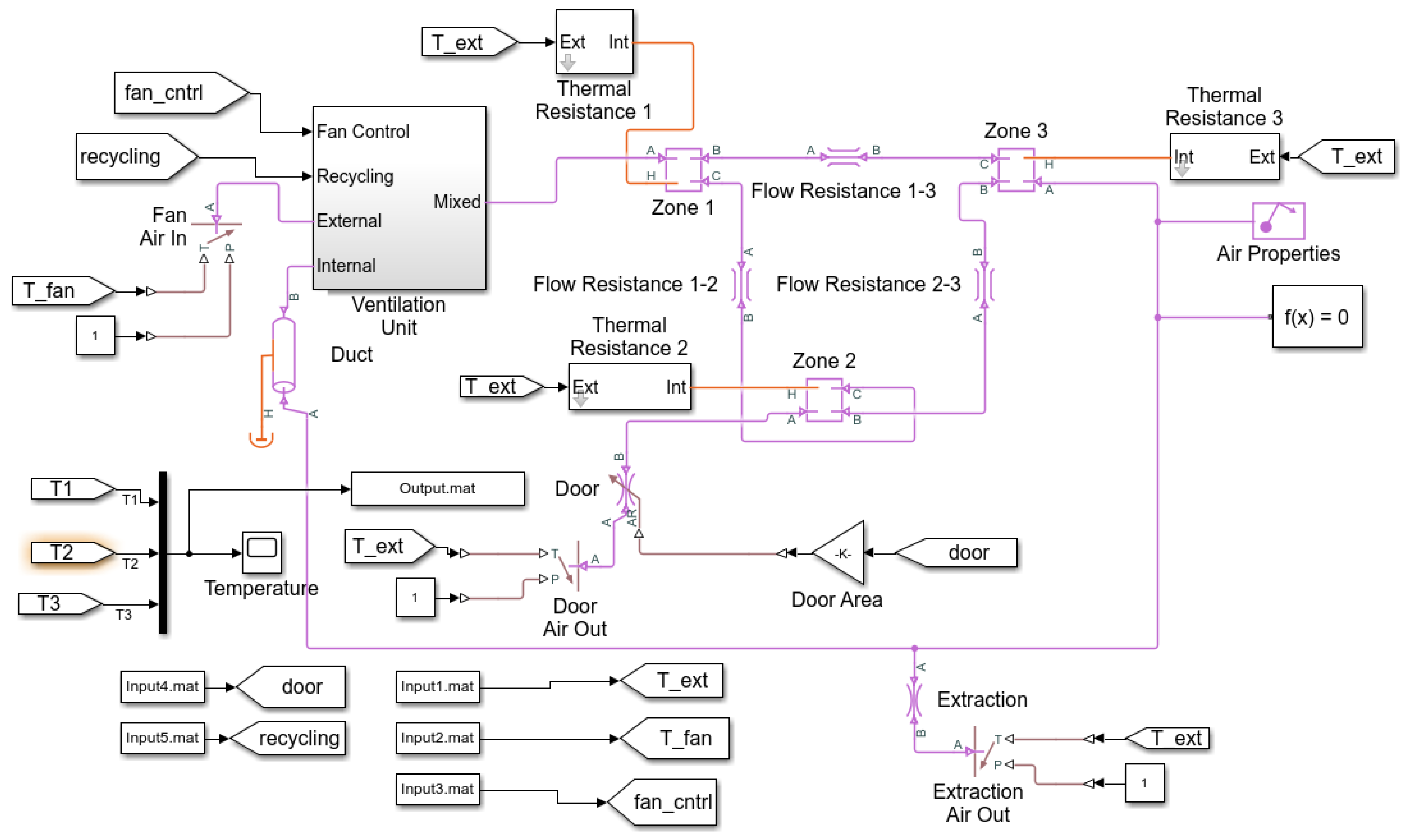
The proposed method in identifying a nonlinear system using a multi-mode approach is tested on a building ventilation system. In this example, the air volume inside the building is divided into three zones. The ventilation unit blows cool air into Zone 1 and exhausts air from Zone 3. The vented air can be optionally recycled back into Zone 1. A door in Zone 2 can be opened to vent air out to the atmosphere. The schematic of the ventilation system is shown in Figure 2.

There are five different types of disturbances in this example, including outdoor and indoor temperature, fan speed, door state and recycling periods. The daily average temperature of Edmonton, Canada, for the last 3 years [16] was used as the simulated outdoor temperature. The NaN (not-a-number) values in outdoor temperature are replaced with the last observed values.

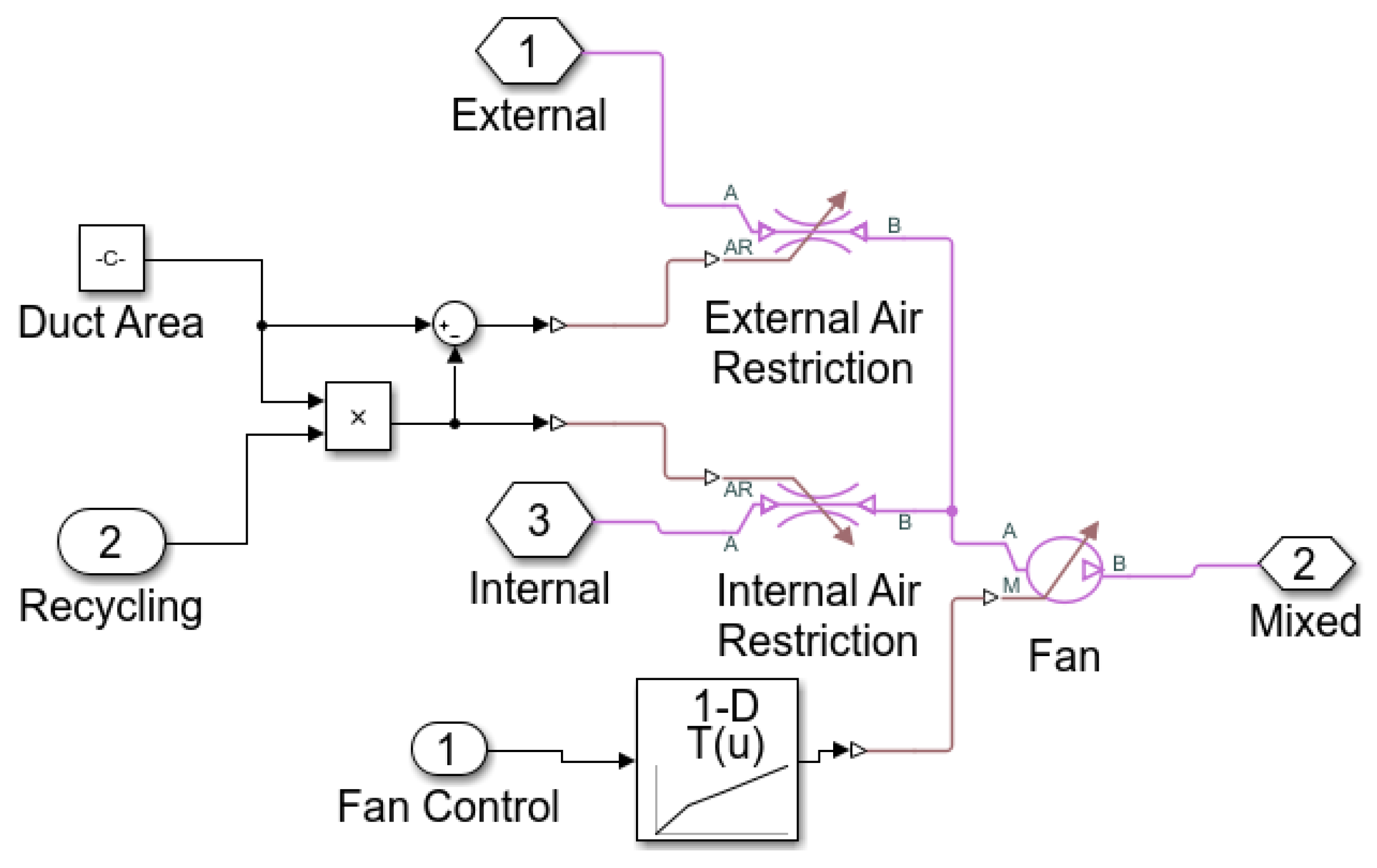
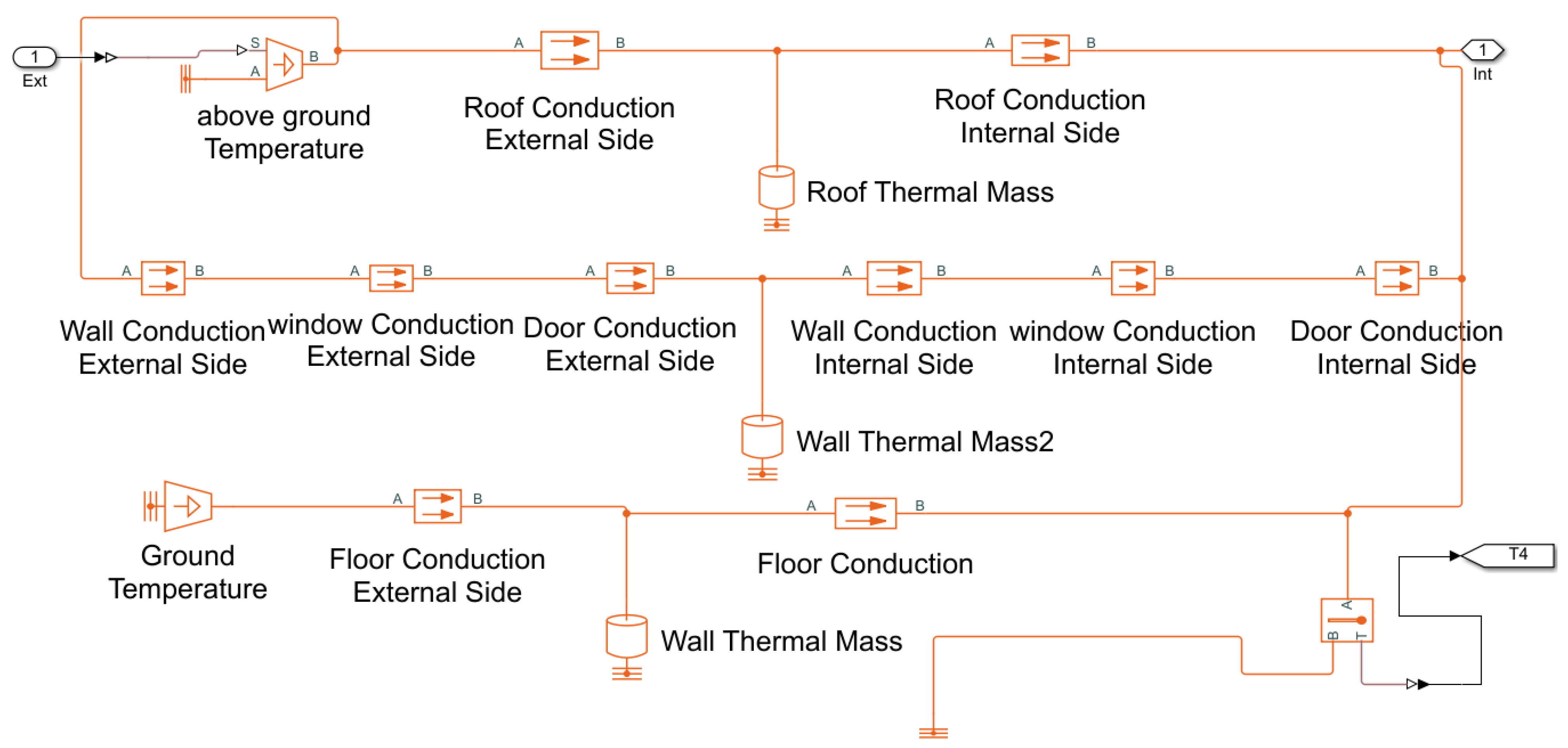
The ventilation system’s outdoor and indoor air characteristics are mixed and blown into the zones are illustrated in Figure 3. In this test, the fan is operated at a fixed speed. The heating resistance of the building is shown in Figure 4. In this test, for each zone, conductive heat transfers from above ground and below the foundation are considered, which are the heat transfers between insides and outsides through windows, doors and walls. The convective heat losses are ignored at this stage phase, which will be addressed in the near future.

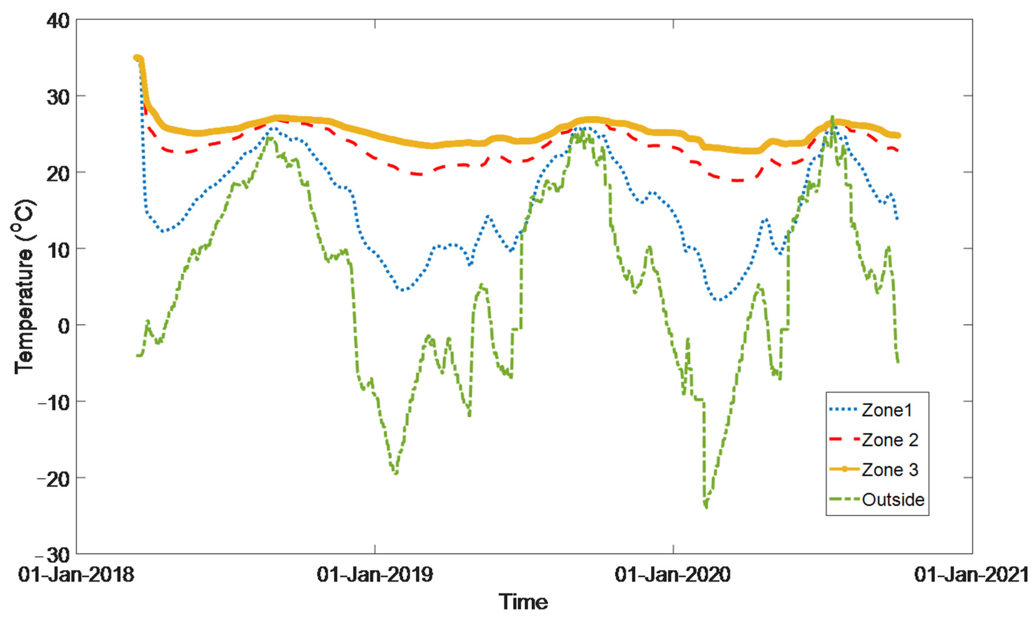
To test the performance of the proposed method, the building ventilation system has been operated in three different operation modes. As seen in Figure 5, the outdoor temperature changes in the range [−25 °C, 25 °C]. This test aims to assess the performance of the proposed identification method in classifying these operation modes and building a multi-mode model for this system. The temperatures at all three zones are illustrated in Figure 5. In this test, the ventilation system does not have pre-heating coils, so the outdoor temperature directly affects the zones temperature. This is why the zones’ temperatures are varying significantly. Therefore, utilizing a pre-heating system before blowing the outdoor air into the zone, especially in cold regions, will produce smoother temperature trends.

The following ARX model structure with 10 models is used in this test.

$$\begin{array}{cc}\hfill Model i:y\left(t+1\right)& \\ & =a_1^{i}y\left(t\right)+a_2^{i}y\left(t-1\right)+a_3^{i}y\left(t-2\right)+b_1^{i}u\left(t-3\right)\hfill \\ & +b_2^{i}u\left(t-4\right)+b_3^{i}u\left(t-5\right) i=1.\cdots .10\hfill \end{array}$$

(10)

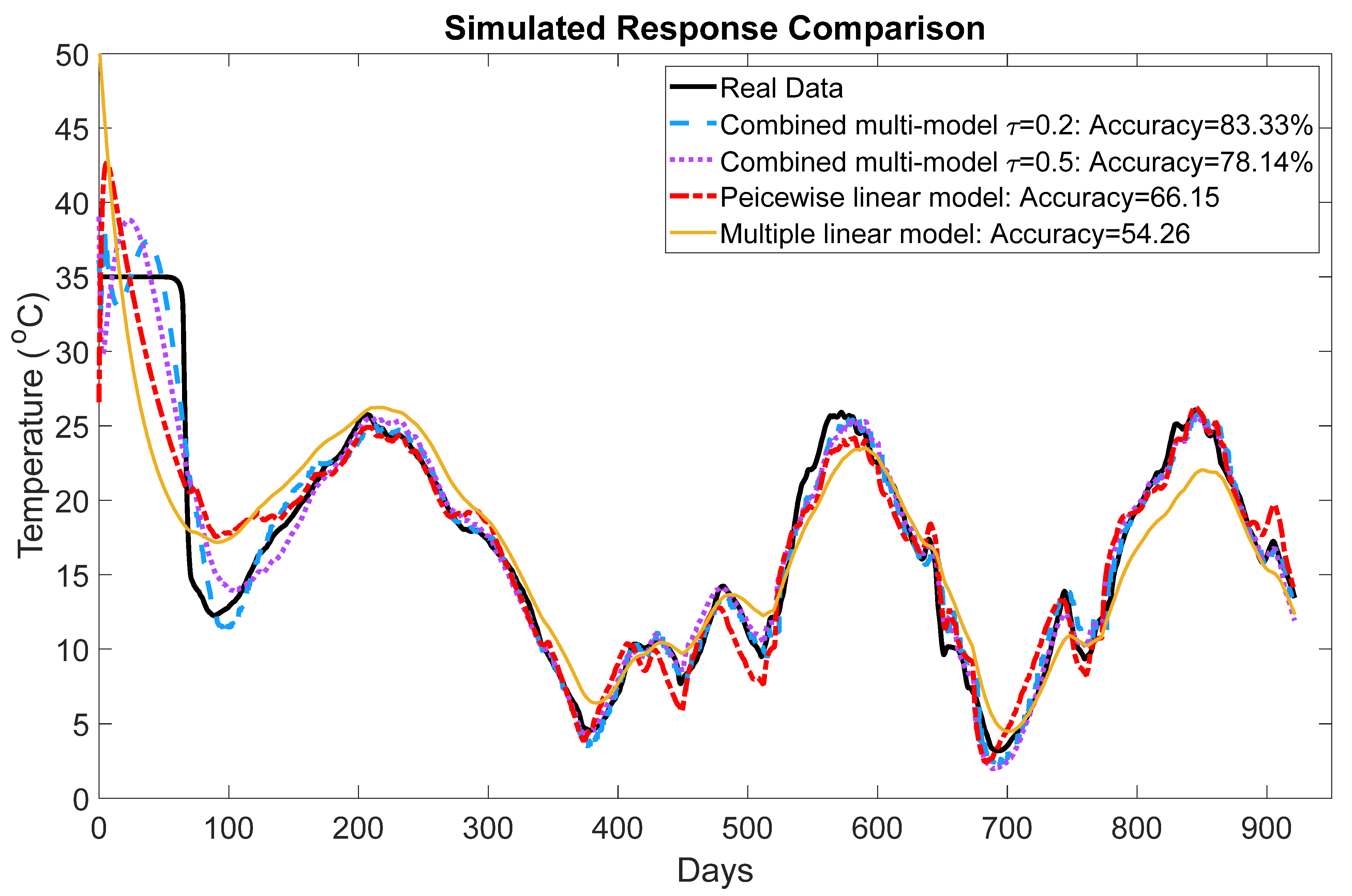
where y(t) denotes indoor temperature at Zone 1, and u(t) denotes the fan temperature, which is almost the same as the outdoor temperature. This model identifies the ventilation behavior with respect to the outdoor temperature changes. The temperature range is divided into 10 equal regions, then the 10 linear models in the form (10) are identified for each region. After identifying the 10 models, the gap-metric method is utilized to remove the unnecessary models (models have similar responses) and decrease the local model numbers. The similarity between models is decided based on the gap metric and threshold level. If the distance between models is less than the threshold level, one of the models will be discarded. Therefore, we can decide the number of models and the accuracy of the multi-model by determining a proper threshold level. A higher value will result in lower accuracy but a less complex model. In this test, to assess the impact of different threshold values, we have selected two different threshold levels τ = 0.2 and τ = 0.5, which results in five and three local models, respectively. The estimated values for these two models’ parameters are given in

Table 1. The model parameters that are identified by the proposed method with τ = 0.2.

	Model Parameters
Cluster	${\mathit{a}}_1^{\mathit{i}}$	${\mathit{a}}_2^{\mathit{i}}$	${\mathit{a}}_3^{\mathit{i}}$	${\mathit{b}}_1^{\mathit{i}}$	${\mathit{b}}_2^{\mathit{i}}$	${\mathit{b}}_3^{\mathit{i}}$
i = 1	2.967	−2.935	0.9676	0.0274	−0.05466	0.02726
i = 2	1.744	−0.7323	−0.0119	−0.08569	0.2612	−0.1751
i = 3	2.304	−1.624	0.3201	0.07934	−0.147	0.06769
i = 4	1.077	0.8135	0.89	−0.0528	0.126	−0.073
i = 5	2.927	−2.855	0.9282	0.0168	−0.0325	0.0157

and

Table 2. The model parameters that are identified by the proposed method with τ = 0.5.

	Model Parameters
Cluster	${\mathit{a}}_1^{\mathit{i}}$	${\mathit{a}}_2^{\mathit{i}}$	${\mathit{a}}_3^{\mathit{i}}$	${\mathit{b}}_1^{\mathit{i}}$	${\mathit{b}}_2^{\mathit{i}}$	${\mathit{b}}_3^{\mathit{i}}$
i = 1	2.967	−2.935	0.9676	0.0274	−0.05466	0.02726
i = 2	1.744	−0.7323	−0.0119	−0.08569	0.2612	−0.1751
i = 3	2.304	−1.624	0.3201	0.07934	−0.147	0.06769

.

After deciding the threshold level and the right number of the local models, the gap metric-based weighting approach introduced in Section 3.2 is used to build the global model. The proposed global models (with τ = 0.2 and τ = 0.5) performances in identifying the ventilation system are compared with the multiple ARX model [17,18] and piecewise linear approach, in which the clustering and regression are done separately [19,20].

Figure 6 illustrates the performance of the identified models on the validation data set. As seen in Figure 6, the proposed method with τ = 0.2 has 83.33% and with τ = 0.5 has 78.14% accuracy on the validation data set, which are higher than two other compared methods. The results admit that combining the two steps of clustering and regression can enhance the overall performance of the identified model.

4.2. Test on Real-World Data

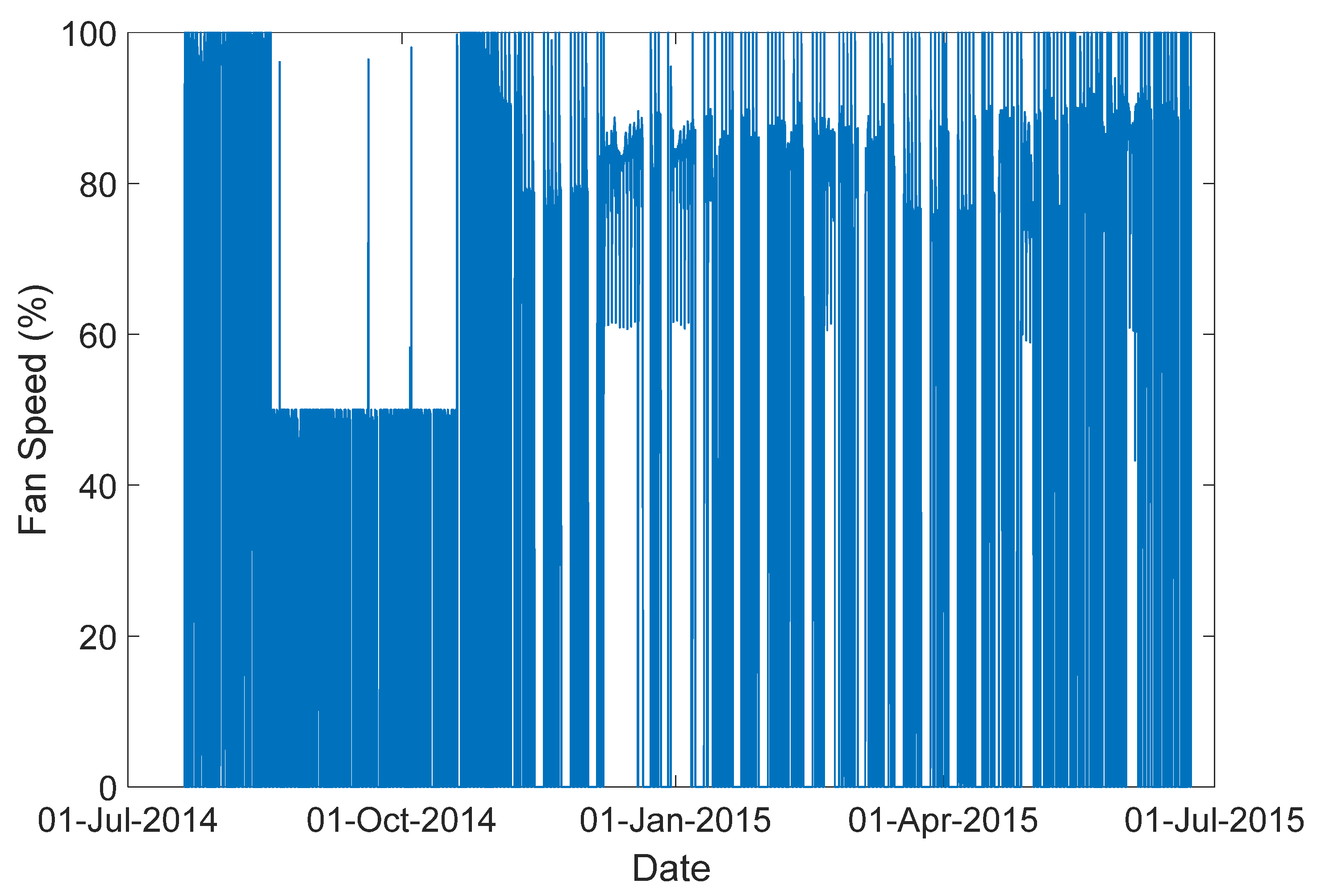
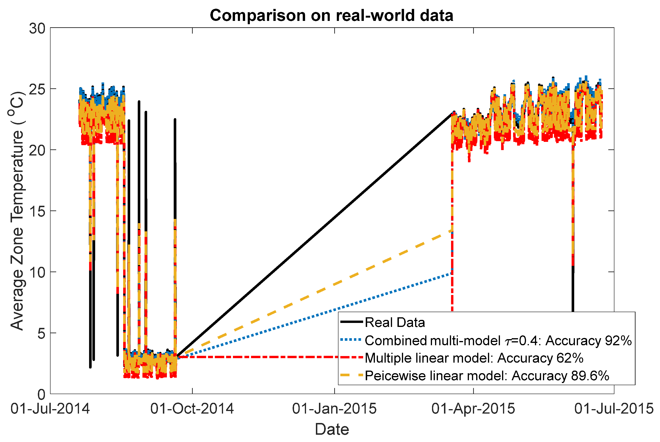
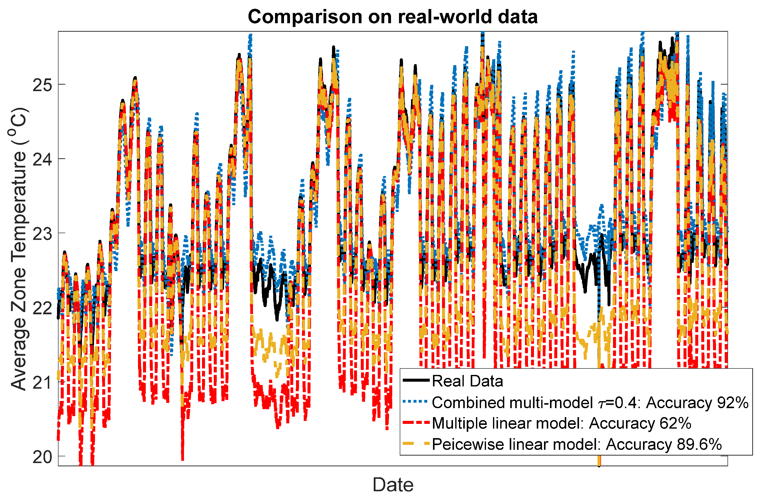
In this section, the proposed modeling approach is tested on real-world data from an office building in Richland, Washington, USA [21]. The dataset includes 378,422 samples for one-year data (from July 2014 to July 2015) of a ventilation system. The inputs and outputs for this system are selected as fan speeds and average zone temperatures, respectively, which are shown in Figure 7 and Figure 8. The system input is selected based on the highest correlation value with the output variable. The proposed method is compared with two other methods introduced above, including the multiple linear model and piecewise linear model. In the proposed method, the temperature region is partitioned into four regions, including 2 to 5 °C, 17 to 20 °C, 20 to 23 °C and 23 to 26 °C; then a local model is identified for each region. Using gap-metric with a threshold level τ = 0.4, all four local models are kept for building the global model. In the piecewise linear model, the same number of local models are considered. To derive the local models and validate the global model, the dataset is divided into two sections, fitting and validating datasets, which are shown in Figure 8. The performance of the three models in predicting 500-step-ahead values is tested on the validation datasets. Figure 9 shows the comparison results. To have a clear view of the model accuracies, the prediction results are magnified in Figure 10. In this comparison, the proposed method has 92% accuracy in predicting the zone temperature, which is higher than the two other methods.

5. Conclusions

One way to identify a nonlinear system such as HVAC with varying operation conditions is to use multi-models. To identify this system using routing operating data, there is a need to cluster each mode’s data and then identify the local models (models for each mode). In this paper, a simultaneous clustering and regression method has been proposed by which a joint cost function is defined and optimized. Furthermore, a gap-metric based method is used to build the global model using the identified local models. The proposed approach has been tested on a simulated and real-world data of ventilation systems. The proposed method outperforms the multiple linear model and the piecewise linear model. The proposed method takes advantage of modeling the system in local regions. The method can capture high nonlinearity and immediate changes in output variables, then use gap-metrics to produce the global model by selecting proper local models and then calculating weights for each selected model.

References

- Abbas, A.; Chowdhury, B. A Data-Driven Approach for Providing Frequency Regulation with Aggregated Residential HVAC Units. In Proceedings of the 2019 IEEE Conference on North American Power Symposium (NAPS), Wichita, KS, USA, 13–15 October 2019. [Google Scholar]
- Khalilnejad, A. Data-Driven Evaluation of HVAC Systems in Commercial Buildings and Identification of Savings Opportunities. Ph.D. Thesis, Case Western Reserve University, Cleveland, OH, USA, 2020. [Google Scholar]
- Yu, X.; Ergan, S.; Dedemen, G. A data-driven approach to extract operational signatures of HVAC systems and analyze impact on electricity consumption. Appl. Energy 2019, 253, 113497. [Google Scholar] [CrossRef]
- Faddel, S.; Tian, G.; Zhou, Q.; Aburub, H. Data Driven Q-Learning for Commercial HVAC Control. In Proceedings of the 2020 SoutheastCon, Raleigh, NC, USA, 28–29 March 2020; pp. 1–6. [Google Scholar] [CrossRef]
- Galan, O.; Romagnoli, J.A.; Palazoglu, A.; Arkun, Y. Gap metric concept and implications for multilinear model-based controller design. Ind. Eng. Chem. Res. 2003, 42, 2189–2197. [Google Scholar] [CrossRef]
- Guay, M. Measurement of Nonlinearity in Chemical Process Control. Ph.D. Thesis, Queen’s University, Kingston, ON, Canada, 1996. [Google Scholar]
- Helbig, A.; Marquardt, W.; Allgower, F. Nonlinearity measures: Definition, computation and applications. J. Process Control 2000, 10, 113–123. [Google Scholar] [CrossRef]
- Nandola, N.N.; Bhartiya, S. A multiple model approach for predictive control of nonlinear hybrid systems. J. Process Control 2008, 18, 131–148. [Google Scholar] [CrossRef]
- Hariprasad, K.; Sharad, B.; Gudi, R.D. A gap metric based multiple model approach for nonlinear switched systems. J. Process Control 2012, 22, 1743–1754. [Google Scholar] [CrossRef]
- Arslan, E.; Çamurdan, M.; Palazoglu, A.; Arkun, Y. Multimodel scheduling control of nonlinear systems using gap metric. Ind. Eng. Chem. Res. 2004, 43, 8275–8283. [Google Scholar] [CrossRef]
- Tan, W.; Marquez, H.J.; Chen, T.; Liu, J. Multimodel analysis and controller design for nonlinear processes. Comput. Chem. Eng. 2004, 28, 2667–2675. [Google Scholar] [CrossRef]
- Du, J.; Song, C.; Li, P. Application of gap metric to model bank determination in multilinear model approach. J. Process Control 2009, 19, 231–240. [Google Scholar] [CrossRef]
- Du, J.; Johansen, T.A. Integrated multimodel control of nonlinear systems based on gap metric and stability margin. Ind. Eng. Chem. Res. 2014, 53, 10206–10215. [Google Scholar] [CrossRef]
- Ben-Hur, A.; Horn, D.; Siegelmann, H.T.; Vapnik, V. Support vector clustering. J. Mach. Learn. Res. 2001, 2, 125–137. [Google Scholar] [CrossRef]
- Available online: https://www.mathworks.com/help/physmod/simscape/ug/building-ventilation.html (accessed on 7 January 2021).
- Available online: https://edmonton.weatherstats.ca/download.html (accessed on 7 January 2021).
- Chi-Man, Y.J.; Wang, S. Multiple ARMAX modeling scheme for forecasting air conditioning system performance. Energy Convers. Manag. 2007, 48, 2276–2285. [Google Scholar]
- Mustafaraj, G.; Chen, J.; Lowry, G. Development of room temperature and relative humidity linear parametric models for an open office using BMS data. Energy Build. 2010, 42, 348–356. [Google Scholar] [CrossRef]
- Benzaama, M.H.; Rajaoarisoa, L.H.; Ajib, B.; Lecoeuche, S. A data-driven methodology to predict thermal behavior of residential buildings using piecewise linear models. J. Build. Eng. 2020, 32, 101523. [Google Scholar] [CrossRef]
- Hure, N.; Vašak, M. Clustering-based identification of mimo piecewise affine systems. In Proceedings of the 2017 21st International Conference on Process Control (PC), Strbske Pleso, Slovakia, 6–9 June 2017. [Google Scholar]
- Available online: https://openei.org/datasets/dataset/long-term-data-on-3-office-air-handling-units (accessed on 7 January 2021).
Figure 1.
Support vector-based clustering (SVC) schematic. Red and black dots belong to cluster 1 and 2, respectively.
Figure 2.
The building ventilation schematic [15].
Figure 3.
The fan control block [15].
Figure 4.
The thermal resistance schematic of the test ventilation system.
Figure 5.
Temperatures at all three zones.
Figure 6.
The performance of the identified models.
Figure 7.
The ventilation system input.
Figure 8.
The ventilation system output.
Figure 9.
Performances of the three models in 500-step ahead prediction of the zone temperature.
Figure 10.
Magnified results of the three models’ performances.