Conservation Integrals in Nonhomogeneous Materials with Flexoelectricity

Abstract

The flexoelectricity, which is a new electromechanical coupling phenomenon between strain gradients and electric polarization, has a great influence on the fracture analysis of flexoelectric solids due to the large gradients near the cracks. On the other hand, although the flexoelectricity has been extensively investigated in recent decades, the study on flexoelectricity in nonhomogeneous materials is still rare, especially the fracture problems. Therefore, in this manuscript, the conservation integrals for nonhomogeneous flexoelectric materials are obtained to solve the fracture problem. Application of operators such as grad, div, and curl to electric Gibbs free energy and internal energy, the energy-momentum tensor, angular momentum tensor, and dilatation flux can also be derived. We examine the correctness of the conservation integrals by comparing with the previous work and discuss the operator method here and Noether theorem in the previous work. Finally, considering the flexoelectric effect, a nonhomogeneous beam problem with crack is solved to show the application of the conservation integrals.

1. Introduction

Unlike the piezoelectric effect only existing in noncentrosymmetric dielectrics, flexoelectricity is an important electromechanical coupling phenomenon theoretically existing in materials with all possible symmetries [1,2]. The main characteristic of the flexoelectricity is that the solids deform due to the electric field gradient and vice versa, they produce electric polarization due to the strain gradient. In recent decades, researchers have researched flexoelectric effects from theories [3,4,5], atomic simulation and molecular dynamics simulation [6,7,8], experimental measurement [9,10,11,12], and device application [13,14,15,16]. For example, from the phenomenological and microscopic perspectives, Tagantsev [17,18] systematically analyzed the flexoelectric effects and piezoelectric effects and provided a method to calculate the values of the flexoelectric coefficients. For nanosized dielectrics, Hu and Shen [3,19], Shen and Hu [4] established the dynamic variational principle for flexoelectric dielectrics with surface effects and obtained generalized governing equations and Young–Laplace equations. However, there have been few studies on the flexoelectric effect introduced by the inhomogeneity of the solids. Besides, flexoelectricity may change the strength and fracture toughness of the material [20] due to the large gradients near the defects. Thus, it is necessary to accurately understand the fracture problems for the flexoelectric solids, further for nonhomogeneous flexoelectric solids.

For classical mechanical or piezoelectric fracture problems, the governing equations and the corresponding boundary conditions are solved directly using the complex potential method [21,22]. However, it is difficult to obtain the exact solutions for some crack problems due to the mathematical complexities. These difficulties urged researchers to obtain the conservation laws or conservation integrals such as J-, M-, and L- integrals to bypass the complexities around the crack tip. J-, M-, and L-integrals are related to the energy release rates for crack translation, crack rotation, and self-similar expansion [23]. Then, the stress intensity factor (SIF) can be obtained naturally from the J-, M-, and L-integrals, which is helpful to study fracture problems. Several methods of constructing conservation integrals can be classified into the following categories:

(i)

The procedure used most widely is Noether theorem. Since Emmy Noether demonstrated the corresponding relation between the conservation integrals and the symmetries in 1918 [24], conservation integrals derived from the Noether theorem have been extensively developed by constructing different symmetries. Usually, according to Noether theorem, J-, M-, and L-integrals can be derived from the corresponding coordinate translation symmetry, scaling symmetry, and coordinate rotation symmetry, respectively. For instance, beginning with these symmetries, Knowles and Sternberg [25], and Fletcher [26], developed conservation laws in elastostatics and linear elastodynamics, respectively. Yang and Batra [27] obtained the conservation laws for linear piezoelectric materials. Other applications of Noether theorem can be found in second gradient electroelasticity [28], flexoelectric solids [29], dissipative electrochemomechanical coupling processes [30,31].

(ii)

The Neutral Action method for dissipative systems or nonhomogeneous solids. It is well known that the classical Noether’s theorem is only applicable to the Lagrangian systems. For systems without a Lagrangian, Honein et al. [32] developed a novel methodology called Neutral Action method to obtain the conservation laws directly from the partial differential equations. Then, their method was used to obtain conservation integrals for nonhomogeneous plane problems [33] and nonhomogeneous Bernoulli–Euler beams [34]. Nordbrock and Kienzer [35] applied the Neutral Action method to Schrödinger equation and found a new conservation law.

(iii)

The third type is called configurational force method or material force method in this manuscript, which originated from the energy-momentum tensor proposed by Eshelby [36]. The procedure is subjecting the Lagrangian density to the differential operators of grad, div, and curl, respectively [37]. Compared with the previous two methods, this method more easily obtains conservation laws for nonhomogeneous materials. For example, Kirchner [38] derived the energy-momentum tensor for nonhomogeneous anisotropic linearly elastic three-dimensional solids. Then, following this procedure, Lazar and Kirchner [39], Kirchner and Lazar [40], obtained the Eshelby stress tensor and conservation laws for gradient elasticity of nonhomogeneous, incompatible, linear, anisotropic media, and bone growth and remodeling, respectively. Recently, Agiasofitou and Lazar studied the elastic dislocations in elasticity [41] and electro-elastic dislocations in piezoelectric materials [42] through the conservation integrals derived from this method.

(iv)

Betti’s reciprocal theorem [43]. The famous application is the Bueckner work conjugate integral [44].

Through these methods, conservation integrals have been extensively developed for many aspects. However, there is almost no literature on conservation integrals in nonhomogeneous flexoelectric solids. Therefore, by adopting the mathematical method of Agiasofitou and Lazar [42] for the derivation of conservation integrals in piezoelectric materials, the aim of this work is systematically constructing the conservation integrals like J-, M-, and L-integrals in nonhomogeneous flexoelectric materials.

The paper is organized as follows. In Section 2, some basic equations in nonhomogeneous flexoelectric materials are listed and reviewed. Based on operator method, conservation integrals are constructed from the electric Gibbs function in Section 3. In Section 4, we similarly obtain conservation integrals from internal energy density. The application of J-integral in a nonhomogeneous beam with crack is illustrated in Section 5. Finally, some conclusions are given in Section 6.

2. Basic Equations in Nonhomogeneous Flexoelectric Materials

The field equations for flexoelectric solids are, with $f_i$ being the body force and ${\rho }_e$ being the free electric charge [45]

$${\sigma }_{ij,j}-{\tau }_{ijm,mj}+f_i=0$$

(1)

$$D_{i,i}-Q_{ij,ji}-{\rho }_e=0$$

(2)

where ${\sigma }_{ij}$, ${\tau }_{ijm}$, $D_i$, and $Q_{ij}$ are the stress, the high-order stress, the electric displacement, and the high-order electric quadrupole, respectively. In this paper, the subscript comma indicates differentiation with respect to the spatial variables, all the derivations are discussed in rectangular Cartesian coordinates and the Latin indices run from 1 to 3.

Using the assumption of linear theory for the flexoelectric solids, the bulk internal energy density function $u$ can be written as [3,4]

$$\begin{array}{l}u=\frac{1}{2}{C}_{ijkl}{\epsilon }_{ij}{\epsilon }_{kl}+r_{ijklm}{\epsilon }_{ij}{w}_{klm}+d_{ijk}{\epsilon }_{ij}{D}_k+e_{ijkl}{\epsilon }_{ij}{Q}_{kl} + \frac{1}{2}{g}_{ijklmn}{w}_{ijk}{w}_{lmn} \\ +\frac{1}{2}{a}_{kl}{D}_k{D}_l+f_{ijkl}{D}_i{w}_{jkl}+{\eta }_{ijkmn}{Q}_{ij}{w}_{kmn}+h_{ijk}{D}_i{Q}_{jk} +\frac{1}{2}{b}_{ijkl}{Q}_{ij}{Q}_{kl}\end{array}$$

(3)

where $C_{ijkl}$, $r_{ijklm}$, $d_{ijk}$, $e_{ijkl}$, $g_{ijklmn}$, $f_{ijkl}$, ${\eta }_{ijkmn}$, $a_{kl}$, $h_{ijk}$, $b_{ijkl}$ are the material coefficients.

Besides, we emphasize that these material coefficients depend on space position for the nonhomogeneous flexoelectric solid studied in this manuscript. $\epsilon$ and $w$ are the strain tensor and the strain gradient tensor, respectively, which are defined as

$${\epsilon }_{ij}=\frac{1}{2}\left(u_{i,j}+u_{j,i}\right), w_{ijm}={\epsilon }_{ij,m}=u_{i,jm}$$

(4)

where $u$ is the displacement vector. Under the infinitesimal deformation assumption, the constitutive equations for the bulk can be expressed in terms of the internal energy as

$$\begin{array}{l}{\sigma }_{ij}=\frac{\partial u}{\partial {\epsilon }_{ij}}=C_{ijkl}{\epsilon }_{kl}+r_{ijklm}{w}_{klm}+d_{ijk}{D}_k+e_{ijkl}{Q}_{kl}\\ {\tau }_{ijm}=\frac{\partial u}{\partial w_{ijm}}=r_{klijm}{\epsilon }_{kl}+g_{ijmknl}{w}_{knl}+f_{kijm}{D}_k+{\eta }_{klijm}{Q}_{kl}\\ E_i=\frac{\partial u}{\partial D_i}=d_{jki}{\epsilon }_{jk}+f_{ijkl}{w}_{jkl}+a_{ij}{D}_j+h_{ijk}{Q}_{jk}\\ V_{ij}=\frac{\partial u}{\partial Q_{ij}}=e_{klij}{\epsilon }_{kl}+{\eta }_{ijkmn}{w}_{kmn}+h_{kij}{D}_k+b_{ijkl}{Q}_{kl}\end{array}$$

(5)

where $E$ is the effective local electric field strength with $E=-\nabla \phi$, $V$ is the electric field gradient tensor with $V=\nabla E$. Using constitutive equations, the bulk internal energy density function $u$ can be rewritten as

$$u=\frac{1}{2}\sigma :\epsilon +\frac{1}{2}\tau ⋮w+\frac{1}{2}E\cdot D+\frac{1}{2}V:Q$$

(6)

Using the Legendre transformation, the electrochemical Gibbs function $g^E$ is

$$g^E=u-E\cdot D-V:Q$$

(7)

Similarly, the bulk electric Gibbs free energy density function $g^E$ can be written as [19]

$$\begin{array}{l}{g}^E=\frac{1}{2}{C}_{ijkl}{\epsilon }_{ij}{\epsilon }_{kl}+r_{ijklm}{\epsilon }_{ij}{w}_{klm}-d_{ijk}{\epsilon }_{ij}{E}_k-e_{ijkl}{\epsilon }_{ij}{V}_{kl}+ \frac{1}{2}{g}_{ijklmn}{w}_{ijk}{w}_{lmn} \\ -f_{ijkl}{E}_i{w}_{jkl}-{\eta }_{ijkmn}{V}_{ij}{w}_{kmn}-\frac{1}{2}{a}_{kl}{E}_k{E}_l-h_{ijk}{E}_i{V}_{jk}-\frac{1}{2}{b}_{ijkl}{V}_{ij}{V}_{kl}\end{array}$$

(8)

Thus, the constitutive equations for the bulk can be expressed in terms of the electric Gibbs free energy as

$$\begin{array}{l}{\sigma }_{ij}=\frac{\partial g^E}{\partial {\epsilon }_{ij}}=C_{ijkl}{\epsilon }_{kl}+r_{ijklm}{w}_{klm}-d_{ijk}{E}_k-e_{ijkl}{V}_{kl}\\ {\tau }_{ijm}=\frac{\partial g^E}{\partial w_{ijm}}=r_{klijm}{\epsilon }_{kl}+g_{ijmknl}{w}_{knl}-f_{kijm}{E}_k-{\eta }_{klijm}{V}_{kl}\\ D_i=-\frac{\partial g^E}{\partial E_i}=d_{jki}{\epsilon }_{jk}+f_{ijkl}{w}_{jkl}+a_{ij}{E}_j+h_{ijk}{V}_{jk}\\ Q_{ij}=-\frac{\partial g^E}{\partial V_{ij}}=e_{klij}{\epsilon }_{kl}+{\eta }_{ijkmn}{w}_{kmn}+h_{kij}{E}_k+b_{ijkl}{V}_{kl}\end{array}$$

(9)

Using constitutive equations, the bulk electric Gibbs free energy density function $g^E$ can be rewritten as

$$g^E=\frac{1}{2}\sigma :\epsilon +\frac{1}{2}\tau ⋮w-\frac{1}{2}D\cdot E-\frac{1}{2}Q:V$$

(10)

Internal energy density and electric Gibbs free energy density can be used to obtain the conservation laws or dual conservation laws [46], which will be obtained in the following sections.

3. Conservation Integrals Relevant to the Electric Gibbs Function

Using translation, scaling, and rotation transformation, Kirchner obtained the energy-momentum tensor and the configurational force (i.e., the corresponding conservation integrals) for nonhomogeneous linear elasticity [38] and gradient elasticity [39]. Yu et al., obtained the path-independent integrals in homogeneous electrochemomechanical materials with flexoelectricity through Noether theorem [31]. In this manuscript, following the procedure of Agiasofitou and Lazar [42] for the derivation of conservation laws for electroelastic dislocations in piezoelectric materials, we aim to obtain J-, M-, and L-integrals in nonhomogeneous flexoelectric materials with body force and free electric charge.

3.1. Application of Translation and J-Integral

Using Equation (10), the total electric Gibbs free energy is

$$G^E={\displaystyle {\int }_V{g}^{E}dV}=\frac{1}{2}{\displaystyle {\int }_V\left(\sigma :\epsilon +\tau ⋮w-D\cdot E-Q:V\right)dV}$$

(11)

Now let us take an arbitrary infinitesimal functional derivative $\delta G^E$ of the energy density. Substituting the constitutive Equation (9) into Equation (11), one can obtain

$$\begin{array}{l}\delta G^E={\displaystyle {\int }_V\delta g^{E}dV}\\ ={\displaystyle {\int }_V\delta \left(\begin{array}{l}\frac{1}{2}{C}_{ijkl}{\epsilon }_{ij}{\epsilon }_{kl}+r_{ijklm}{\epsilon }_{ij}{w}_{klm}-d_{ijk}{\epsilon }_{ij}{E}_k-e_{ijkl}{\epsilon }_{ij}{V}_{kl}+ \frac{1}{2}{g}_{ijklmn}{w}_{ijk}{w}_{lmn} \\ -f_{ijkl}{E}_i{w}_{jkl}-{\eta }_{ijkmn}{V}_{ij}{w}_{kmn}-\frac{1}{2}{a}_{kl}{E}_k{E}_l-h_{ijk}{E}_i{V}_{jk}-\frac{1}{2}{b}_{ijkl}{V}_{ij}{V}_{kl}\end{array}\right)dV}\end{array}$$

(12)

In the following, the functional derivative will be converted to be translational

$$\delta =\left(\delta x_k\right)\frac{\partial }{\partial x_k}=\left(\delta x_k\right){\partial }_k$$

(13)

Using Equation (13), one can get from the left-hand side of Equation (12)

$$\delta G^E={\displaystyle {\int }_V\delta g^{E}dV}={\displaystyle {\int }_V\left({\partial }_k{g}^E\right)\left(\delta x_k\right)dV}={\displaystyle {\int }_V{\partial }_i\left(g^E{\delta }_{ik}\right)\left(\delta x_k\right)dV}$$

(14)

Considering that the material coefficients are also the function of the space coordinates and using the symmetry of these material coefficients, the integrand in the second integral in Equation (12) can be derived as follows

$$\begin{array}{ll}\delta \left(g^E\right) & =\frac{1}{2}\left[{\partial }_k{C}_{ijkl}\right]{\epsilon }_{ij}{\epsilon }_{kl}\delta x_k+\left[{\partial }_k{r}_{ijklm}\right]{\epsilon }_{ij}{w}_{klm}\delta x_k\\ & -\left[{\partial }_k{d}_{ijk}\right]{\epsilon }_{ij}{E}_k\delta x_k-\left[{\partial }_k{e}_{ijkl}\right]{\epsilon }_{ij}{V}_{kl}\delta x_k + \frac{1}{2}\left[{\partial }_k{g}_{ijklmn}\right]w_{ijk}{w}_{lmn}\delta x_k\\ & -\left[{\partial }_k{f}_{ijkl}\right]E_i{w}_{jkl}\delta x_k-\left[{\partial }_k{\eta }_{ijkmn}\right]V_{ij}{w}_{kmn}\delta x_k\\ & -\frac{1}{2}\left[{\partial }_k{a}_{kl}\right]E_k{E}_l\delta x_k-\left[{\partial }_k{h}_{ijk}\right]E_i{V}_{jk}\delta x_k-\frac{1}{2}\left[{\partial }_k{b}_{ijkl}\right]V_{ij}{V}_{kl}\delta x_k\\ & +{\sigma }_{ij}\left[\delta {\epsilon }_{ij}\right]+{\tau }_{ijm}\left[\delta w_{ijm}\right]-D_i\left[\delta E_i\right]-Q_{ij}\left[\delta V_{ij}\right]\\ & =A_k^G\delta x_k+{\sigma }_{ij}\left[\delta {\epsilon }_{ij}\right]+{\tau }_{ijm}\left[\delta w_{ijm}\right]-D_i\left[\delta E_i\right]-Q_{ij}\left[\delta V_{ij}\right]\end{array}$$

(15)

For convenience, mark the first four lines in Equation (15) as $A_k^G\delta x_k$ with

$$\begin{array}{l}{A}_k^G=\frac{1}{2}\left[{\partial }_k{C}_{ijkl}\right]{\epsilon }_{ij}{\epsilon }_{kl}+\left[{\partial }_k{r}_{ijklm}\right]{\epsilon }_{ij}{w}_{klm} -\left[{\partial }_k{d}_{ijk}\right]{\epsilon }_{ij}{E}_k\\ -\left[{\partial }_k{e}_{ijkl}\right]{\epsilon }_{ij}{V}_{kl} + \frac{1}{2}\left[{\partial }_k{g}_{ijklmn}\right]w_{ijk}{w}_{lmn} -\left[{\partial }_k{f}_{ijkl}\right]E_i{w}_{jkl}\\ -\left[{\partial }_k{\eta }_{ijkmn}\right]V_{ij}{w}_{kmn}-\frac{1}{2}\left[{\partial }_k{a}_{kl}\right]E_k{E}_l-\left[{\partial }_k{h}_{ijk}\right]E_i{V}_{jk}-\frac{1}{2}\left[{\partial }_k{b}_{ijkl}\right]V_{ij}{V}_{kl}\end{array}$$

(16)

Thus, $A_k^G$ is the so-called material inhomogeneity force which represents the nonhomogeneous property of the material.

The following derivation can be obtained for the terms in the last line in Equation (15)

$${\sigma }_{ij}\left[\delta {\epsilon }_{ij}\right]={\sigma }_{ij}\left[{\partial }_k{\epsilon }_{ij}\right]\left(\delta x_k\right)=\left[{\left({\sigma }_{ij}{u}_{i,k}\right)}_{,j}-{\sigma }_{ij,j}{u}_{i,k}\right]\left(\delta x_k\right)$$

(17)

$$\begin{array}{l}{\tau }_{ijm}\left[\delta w_{ijm}\right]={\tau }_{ijm}\left[{\partial }_k{w}_{ijm}\right]\left(\delta x_k\right) \\ =\left[{\left({\tau }_{ijm}{u}_{i,jk}\right)}_{,m}-{\tau }_{ijm,m}{u}_{i,jk}\right]\left(\delta x_k\right)\\ =\left\{{\left({\tau }_{ijm}{u}_{i,jk}\right)}_{,m}-\left[{\left({\tau }_{ijm,m}{u}_{i,k}\right)}_{,j}-{\tau }_{ijm,mj}{u}_{i,k}\right]\right\}\left(\delta x_k\right)\\ =\left[{\left({\tau }_{ijm}{u}_{i,jk}\right)}_{,m}-{\left({\tau }_{ijm,m}{u}_{i,k}\right)}_{,j}+{\tau }_{ijm,mj}{u}_{i,k}\right]\left(\delta x_k\right)\end{array}$$

(18)

$$\begin{array}{l}{D}_i\left(\delta E_i\right)=D_i{\partial }_k{E}_i\delta x_k=D_i\left({\partial }_i{E}_k\right)\delta x_k\\ =\left[{\partial }_i\left(D_i{E}_k\right)-\left({\partial }_i{D}_i\right)E_k\right]\delta x_k=-\left[{\partial }_i\left(D_i{\phi }_{,k}\right)-\left({\partial }_i{D}_i\right){\phi }_{,k}\right]\delta x_k\end{array}$$

(19)

$$\begin{array}{l}{Q}_{ij}\left[\delta V_{ij}\right]=Q_{ij}\left[{\partial }_k{V}_{ij}\right]\left(\delta x_k\right)\\ =-Q_{ij}{\phi }_{,ijk}\left(\delta x_k\right)=-\left[{\left(Q_{ij}{\phi }_{,ik}\right)}_{,j}-Q_{ij,j}{\phi }_{,ik}\right]\left(\delta x_k\right)\\ =-\left[{\left(Q_{ij}{\phi }_{,ik}\right)}_{,j}-{\left(Q_{ij,j}{\phi }_{,k}\right)}_{,i}+Q_{ij,ji}{\phi }_{,k}\right]\left(\delta x_k\right)\end{array}$$

(20)

Substituting Equations (14)–(20)and governing Equations (1) and (2) into Equation (12), one can get

$$\begin{array}{l}{\displaystyle {\int }_V{\partial }_i\left[g^E{\delta }_{ik}-{\sigma }_{ij}{u}_{j,k}-{\tau }_{mji}{u}_{m,jk}+{\tau }_{jim,m}{u}_{j,k}-D_i{\phi }_{,k}-Q_{ji}{\phi }_{,jk}+Q_{ij,j}{\phi }_{,k}\right]dV}\\ ={\displaystyle {\int }_V\left(A_k^G+f_i{u}_{i,k}+{\rho }_e{\phi }_{,k}\right)dV}=J_k^G\end{array}$$

(21)

The integrand in the second integral in Equation (21) is the configurational force, which can be defined as

$$F_k=A_k^G+f_i{u}_{i,k}+{\rho }_e{\phi }_{,k}$$

(22)

There are three terms in the configurational force: the first term represents the inhomogeneity of the material, the second term is the configurational force on the body force which can be found in Cherepanov’s work [47], and the third term is the configurational force due to the free electric charge, which is the electrostatic part of the Lorentz force [48].

The integrand in the first integral in Equation (21) is the divergence of the generalized Eshelby stress tensor of nonhomogeneous flexoelectric solid, which is defined as

$$P_{ik}=g^E{\delta }_{ik}-{\sigma }_{ij}{u}_{j,k}-{\tau }_{mji}{u}_{m,jk}+{\tau }_{jim,m}{u}_{j,k}-D_i{\phi }_{,k}-Q_{ji}{\phi }_{,jk}+Q_{ij,j}{\phi }_{,k}$$

(23)

The above generalized energy-momentum tensor can reduce to the conventional elastic Eshelby stress tensor [36], the electroelastic Eshelby stress tensor [49,50]. Based on Equation (21), the relation between the Eshelby stress tensor and the configurational force is

$${\partial }_i{P}_{ik}=F_k$$

(24)

Analogous to governing Equation (1) in classical mechanics in physical space, the above expression is the governing equation in configurational mechanics in material space [51].

Besides, using Gauss divergence theorem in Equation (21), one can find

$$J_k^G={\displaystyle {\int }_V{\partial }_i{P}_{ik}dV}={\displaystyle {\int }_S{n}_i{P}_{ik}dS}$$

(25)

Thus, $J_k^G$ is the J-integral of the nonhomogeneous flexoelectric material, and its value does not equal zero which means this integral is not path-independent. In absence of body force and free electric charge, a path-independent integral $G_k$ can be obtained by moving the inhomogeneity term to the left side in Equation (21),

$$G_k^J=J_k^G-{\displaystyle {\int }_V{A}_k^{G}dV}$$

(26)

Furthermore, if the flexoelectric material is homogeneous, the path-independent integral $G_k^J$ will reduce to the J-integral derived from Noether theorem for homogeneous material in [30].

3.2. Application of Dilatation and M-Integral

If we specify the functional derivative to be dilatational, i.e.,

$$\delta =x_k{\partial }_k$$

(27)

Using the same manipulations, one finds

$$x_k{J}_k^G={\displaystyle {\int }_V{x}_k{F}_{k}dV}={\displaystyle {\int }_V{x}_k{\partial }_i{P}_{ik}dV}={\displaystyle {\int }_V\left[{\partial }_i\left(x_k{P}_{ik}\right)-P_{kk}\right]dV}$$

(28)

with

$$\begin{array}{l}{P}_{kk}=g^E{\delta }_{kk}-{\sigma }_{kj}{u}_{j,k}-{\tau }_{mjk}{u}_{m,jk}+{\tau }_{jkm,m}{u}_{j,k}-D_k{\phi }_{,k}-Q_{jk}{\phi }_{,jk}+Q_{kj,j}{\phi }_{,k}\\ =\frac{n}{2}{\left({\tau }_{ijl}{u}_{i,j}\right)}_{,l}+\frac{n-2}{2}{\left[\left({\sigma }_{ij}-{\tau }_{ijm,m}\right)u_i\right]}_{,j}+\frac{n-2}{2}{f}_i{u}_i-{\tau }_{mjk}{u}_{m,jk}\\ +\frac{n}{2}{\left(Q_{ij}{\phi }_{,j}\right)}_{,i}+\frac{n-2}{2}{\left[\left(D_i-Q_{ij,j}\right)\phi \right]}_{,i}-\frac{n-2}{2}{\rho }_e\phi -Q_{jk}{\phi }_{,jk}\end{array}$$

(29)

where $n$ is the dimension of spatial coordinates. The generalized M-integral for the nonhomogeneous flexoelectric medium with body force and free electric charge is

$$\begin{array}{l}{M}^G={\displaystyle {\int }_V\left[x_k{F}_k+\frac{n-2}{2}{f}_i{u}_i-{\tau }_{mjk}{u}_{m,jk}-\frac{n-2}{2}{\rho }_e\phi +Q_{jk}{\phi }_{,jk}\right]dV}\\ ={\displaystyle {\int }_V{\partial }_i\left\{x_k{P}_{ik}-\frac{n}{2}\left({\tau }_{mji}{u}_{m,j}+Q_{ij}{\phi }_{,j}\right)-\frac{n-2}{2}\left[\left({\sigma }_{ji}-{\tau }_{jim,m}\right)u_j+\left(D_i-Q_{ij,j}\right)\phi \right]\right\}dV}\end{array}$$

(30)

Define the dilatation flux as

$$Y_i=x_k{P}_{ik}-\frac{n}{2}\left({\tau }_{mji}{u}_{m,j}+Q_{ij}{\phi }_{,j}\right)-\frac{n-2}{2}\left[\left({\sigma }_{ji}-{\tau }_{jim,m}\right)u_j+\left(D_i-Q_{ij,j}\right)\phi \right]$$

(31)

Thus, the second integral in Equation (30) can be transformed into a surface integral

$$M^G={\displaystyle {\int }_V{\partial }_i{Y}_{i}dV}={\displaystyle {\int }_S{n}_i{Y}_{i}dS}$$

(32)

It can be easy to draw the conclusion from the first integral in Equation (30) that M-integral derived here is not conserved. In absence of body force and free electric charge, a path-independent integral $G^M$ can be obtained by moving the inhomogeneity term and the gradient term to the left side in Equation (30),

$$G^M=M^G-{\displaystyle {\int }_V\left[x_k{A}_k^G-{\tau }_{mjk}{u}_{m,jk}+Q_{jk}{\phi }_{,jk}\right]dV}$$

(33)

Furthermore, we neglect the gradient terms in a homogeneous medium, M-integral will reduce to

$$M^G={\displaystyle {\int }_S{n}_i\left[x_k\left(g^E{\delta }_{ik}-{\sigma }_{ij}{u}_{j,k}-D_i{\phi }_{,k}\right)-\frac{n-2}{2}\left({\sigma }_{ji}{u}_j+D_i\phi \right)\right]dS}$$

(34)

It is in agreement with the M-integral for elastostatics [25,52] and electroelastic medium [53].

3.3. Application of Rotation and L-Integral

In this part, the functional derivative will be specified to be rotational, i.e.,

$$\delta =\left(\delta x_k\right){\in }_{kji}{x}_j{\partial }_i$$

(35)

So using Equation (25), one can obtain

$${\in }_{kji}{x}_j{J}_i^G={\displaystyle {\int }_V{\in }_{kji}{x}_j{F}_{i}dV}={\displaystyle {\int }_V{\in }_{kji}\left[{\partial }_n\left(x_j{P}_{in}\right)-P_{ij}\right]dV}$$

(36)

The second term in the second integral can be rewritten as

$$\begin{array}{l}{\in }_{kji}{P}_{ij}=-{\in }_{kji}\left({\sigma }_{ik}{u}_{k,j}+{\tau }_{mki}{u}_{m,kj}-{\tau }_{kim,m}{u}_{k,j}+D_i{\phi }_{,j}+Q_{ki}{\phi }_{,kj}-Q_{ik,k}{\phi }_{,j}\right)\\ =-{\in }_{kji}\left\{{\left[\left({\sigma }_{in}-{\tau }_{nim,m}\right)u_i\right]}_{,n}-f_i{u}_j+{\partial }_n\left({\tau }_{mni}{u}_{m,j}\right)-u_{m,j}\left({\partial }_n{\tau }_{mni}\right)\right\}\\ -{\in }_{kji}\left(D_i{\phi }_{,j}+Q_{ki}{\phi }_{,kj}-Q_{ik,k}{\phi }_{,j}\right)\\ =-{\in }_{kji}\left\{{\left[\left({\sigma }_{in}-{\tau }_{nim,m}\right)u_i\right]}_{,n}-f_i{u}_j+{\partial }_n\left({\tau }_{mni}{u}_{m,j}\right)-u_{m,j}\left({\partial }_n{\tau }_{mni}\right)\right\}\\ -{\in }_{kji}\left[D_i{\phi }_{,j}-{\left(Q_{in}{\phi }_{,j}\right)}_{,n}\right]\end{array}$$

(37)

During derivation the above equation, the following relation was used

$${\in }_{kji}{\phi }_{,kj}=0$$

(38)

Thus, substituting Equation (37) into Equation (36) and making some proper rearrangement, one can finally get

$$\begin{array}{l}{\displaystyle {\int }_V{\in }_{kji}\left[x_j{F}_i+f_i{u}_j+u_{m,j}\left({\partial }_n{\tau }_{mni}\right)-D_i{\phi }_{,j}\right]dV}\\ ={\displaystyle {\int }_V{\in }_{kji}{\partial }_n\left[x_j{P}_{in}+\left({\sigma }_{in}-{\tau }_{nim,m}\right)u_i+{\tau }_{mni}{u}_{m,j}-Q_{in}{\phi }_{,j}\right]dV}\end{array}$$

(39)

The integrand of the second integral in Equation (39) is the divergence of the angular momentum tensor

$${\mathsf{\Gamma }}_{kn}={\in }_{kji}\left[x_j{P}_{in}+\left({\sigma }_{in}-{\tau }_{nim,m}\right)u_i+{\tau }_{mni}{u}_{m,j}-Q_{in}{\phi }_{,j}\right]$$

(40)

Then, the L-integral can be expressed as

$$L_k^G={\displaystyle {\int }_S{\mathsf{\Gamma }}_{kj}{n}_{j}dS}$$

(41)

As the configurational moments break the rotational symmetry, the L-integral is not conserved. Without body force and free electric charge, a path-independent integral $G_k^L$ can be obtained from Equation (39)

$$G_k^L=L_k^G-{\displaystyle {\int }_V{\in }_{kji}\left[x_j{A}_i^G+u_{m,j}\left({\partial }_n{\tau }_{mni}\right)-D_i{\phi }_{,j}\right]dV}$$

(42)

4. Conservation Integrals Derived from the Internal Energy

In the previous section, several conservation integrals were obtained from the electric Gibbs free energy with the independent state variables $\left({\epsilon }_{ij},w_{ijk},E_i,V_{ij}\right)$. While in some situations, it is convenient to study the system through internal energy density function when the independent variables are $\left({\epsilon }_{ij},w_{ijk},D_i,Q_{ij}\right)$. Therefore, it is also essential to get the corresponding dual conservation integrals from the internal energy, which are presented as follows without the procedure of derivation.

The total internal energy is

$$U={\displaystyle {\int }_{V}udV}=\frac{1}{2}{\displaystyle {\int }_V(\sigma :\epsilon +\tau ⋮w+E\cdot D+V:Q)dV}$$

(43)

Specifying the functional derivative to be translational, dilatational, and rotational, respectively, the corresponding J-, M-, and L-integrals will be obtained.

(1)

J-integral

One can get

$${\displaystyle {\int }_V{\partial }_i{P}_{ik}dV}={\displaystyle {\int }_V\left(B_k^U+f_i{u}_{i,k}+\phi {\partial }_k{\rho }_e\right)dV}=J_k^U$$

(44)

with

$$\begin{array}{l}{B}_k^U=\frac{1}{2}\left({\partial }_k{C}_{ijkl}\right){\epsilon }_{ij}{\epsilon }_{kl}+\left({\partial }_k{r}_{ijklm}\right){\epsilon }_{ij}{w}_{klm}+\left({\partial }_k{d}_{ijk}\right){\epsilon }_{ij}{D}_k\\ +\left({\partial }_k{e}_{ijkl}\right){\epsilon }_{ij}{Q}_{kl} + \frac{1}{2}\left({\partial }_k{g}_{ijklmn}\right)w_{ijk}{w}_{lmn}+\frac{1}{2}\left({\partial }_k{a}_{kl}\right)D_k{D}_l\\ +\left({\partial }_k{f}_{ijkl}\right)D_i{w}_{jkl}+\left({\partial }_k{\eta }_{ijkmn}\right)Q_{ij}{w}_{kmn}+\left({\partial }_k{h}_{ijk}\right)D_i{Q}_{jk}+\frac{1}{2}\left({\partial }_k{b}_{ijkl}\right)Q_{ij}{Q}_{kl}\end{array}$$

(45)

$$P_{ik}=u{\delta }_{ik}-{\sigma }_{ji}{u}_{j,k}-{\tau }_{mji}{u}_{m,jk}+{\tau }_{jim,m}{u}_{j,k}+D_{i,k}\phi +Q_{ji,k}{\phi }_{,j}-Q_{ij,jk}\phi$$

(46)

here, $B_k^U$ represents the inhomogeneity of the material, $P_{ik}$ is the generalized energy-momentum tensor. Obviously, due to the body force, free electric charge, gradient term, and inhomogeneity of material, the generalized J-integral is not path-independent. However, one can construct a conservation integral as

$$U_k^J=J_k^U-{\displaystyle {\int }_V\left(B_k^U+f_i{u}_{i,k}+\phi {\partial }_k{\rho }_e\right)dV}$$

(47)

(2)

M-integral

Similarly, the M-integral derived from internal energy is

$$M^U={\displaystyle {\int }_V\left[x_k{F}_k+\frac{n-2}{2}{f}_i{u}_i-{\tau }_{mjk}{u}_{m,jk}-\frac{n+2}{2}{\rho }_e\phi -Q_{jk,k}{\phi }_{,j}\right]dV}={\displaystyle {\int }_V{\partial }_i{Y}_{i}dV}$$

(48)

where $Y_i$ is the dilatation flux and

$$Y_i=x_k{P}_{ik}-\frac{n}{2}\left({\tau }_{mji}{u}_{m,j}-Q_{ji}{\phi }_{,j}\right)-\frac{n-2}{2}\left({\sigma }_{ji}-{\tau }_{jim,m}\right)u_j+\frac{n}{2}\left(D_i-Q_{ik,k}\right)\phi$$

(49)

(3)

L-integral

The L-integral can finally be obtained as follows

$$L_k^U={\displaystyle {\int }_S{\mathsf{\Gamma }}_{kj}{n}_{j}dS}={\displaystyle {\int }_V{\in }_{kji}\left[x_j{F}_i+f_i{u}_j+u_{m,j}\left({\partial }_n{\tau }_{mni}\right)-D_{i,j}\phi \right]dV}$$

(50)

with the angular momentum tensor ${\mathsf{\Gamma }}_{kn}$ defined as

$${\mathsf{\Gamma }}_{kn}={\in }_{kji}\left[x_j{P}_{in}+\left({\sigma }_{in}-{\tau }_{nim,m}\right)u_i+{\tau }_{mni}{u}_{m,j}-Q_{in,j}\phi \right]$$

(51)

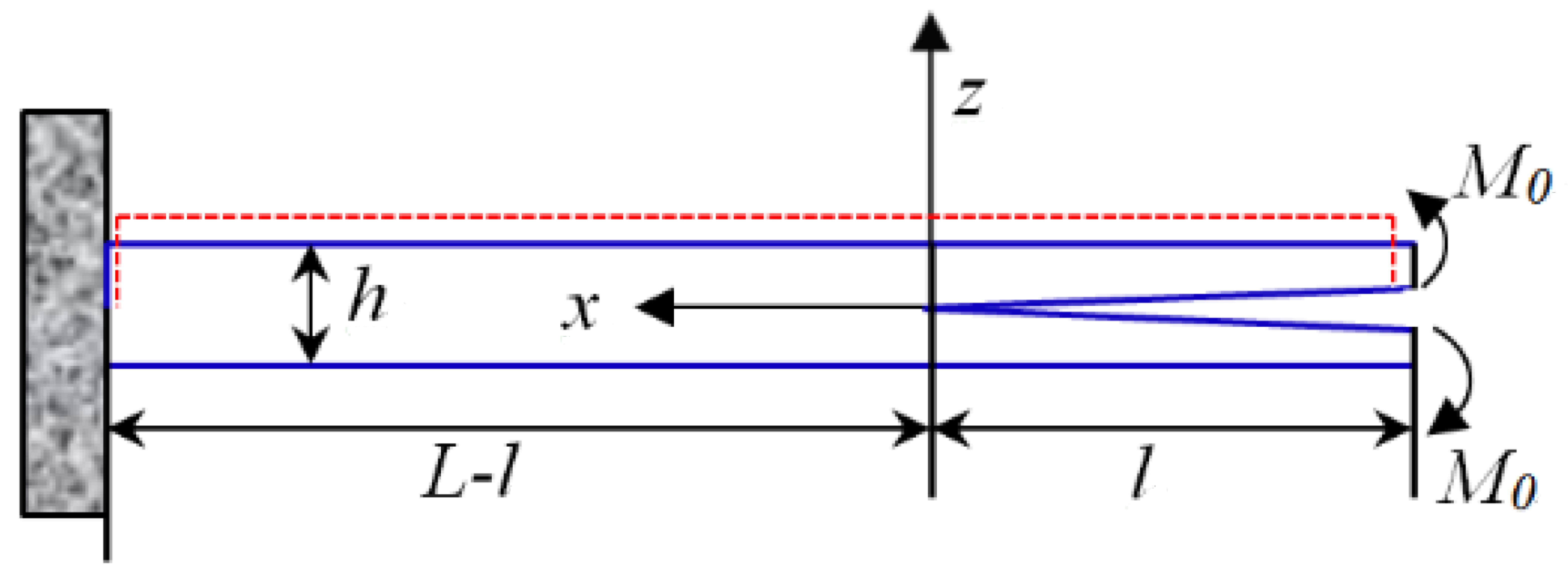
5. A Nonhomogeneous Bernoulli–Euler Beam Problem with Flexoelectricity

In this section, a nonhomogeneous Bernoulli–Euler beam problem will be solved to illustrate the use of the J-integral derived in the previous section. A series of work has been carried out on the Bernoulli–Euler beam [54,55,56,57]. Based on their work, a double cantilever beam problem with a crack loaded by a couple $M_0$ at the free end and the open circuit condition will be solved. Using the coordinate system $\left(x,y,z\right)$ shown in Figure 1, the displacement components can be obtained as follows [58,59],

$$u_x=-z\frac{\partial \upsilon }{\partial x}, u_y=0, u_z=\upsilon$$

(52)

The elastic strain and the strain gradient can be obtained from Equation (52) as

$${\epsilon }_{xx}=-z\frac{d^2\upsilon }{d{x}^2} w_{xxx}=-z\frac{d^3\upsilon }{d{x}^3} w_{xxz}=-\frac{d^2\upsilon }{d{x}^2}$$

(53)

The one-dimensional constitutive equations can be expressed as follows:

$$\begin{array}{l}{\sigma }_{xx}=\frac{\partial g^E}{\partial {\epsilon }_{ij}}=C_{11}{\epsilon }_{xx}-d_{31}{E}_z+\frac{1}{2}{\mu }_{31}{E}_{z,z}\\ {\tau }_{xxz}=\frac{\partial g^E}{\partial w_{ijm}}=-\frac{1}{2}{\mu }_{31}{E}_z\\ D_z=a_{33}{E}_z+d_{31}{\epsilon }_{xx}+\frac{1}{2}{\mu }_{31}{\epsilon }_{xx,z}\\ Q_{zz}=-\frac{1}{2}{\mu }_{31}{\epsilon }_{xx}\end{array}$$

(54)

where ${\mu }_{31}=f_{31}-e_{31}$. It should be stressed that all the material coefficients depend on space position. In this example, for the convenience of mathematical calculations, all the material coefficients take the form:

$$\mathsf{\Omega }={\mathsf{\Omega }}_0{e}^{\alpha x}$$

(55)

where ${\mathsf{\Omega }}_0$ and $\alpha$ are constant. This form can also be found in previous works [51,60].

The electric governing equation is:

$$D_{i,i}-Q_{ij,ji}=0$$

(56)

The electric boundary conditions are assumed as:

$$\phi \left(\frac{1}{2}h\right)=V, \phi \left(-\frac{1}{2}h\right)=0, Q_{33}\left(\pm \frac{1}{2}h\right)=0$$

(57)

Thus, combining Equations (54), (56), and (57), the electric potential, the electric field strength, and electric field gradient can be obtained:

$$\phi \left(z\right)=\frac{V}{2}+\frac{Vz}{h}+\frac{d_{31}}{2a_{33}}\left(\frac{h^2}{4}-z^2\right)\frac{d^2\upsilon }{d{x}^2} -\frac{{\mu }_{31}z}{2a_{33}}\frac{d^2\upsilon }{d{x}^2}$$

(58)

$$E_z=\frac{V}{h}-z\frac{d_{31}}{a_{33}}\frac{d^2\upsilon }{d{x}^2} -\frac{{\mu }_{31}}{2a_{33}}\frac{d^2\upsilon }{d{x}^2}$$

(59)

$$E_{z,z}=-\frac{d_{31}}{a_{33}}\frac{d^2\upsilon }{d{x}^2}$$

(60)

Substituting Equations (58)–(60) into Equation (54), the stress and higher-order stress are:

$$\begin{array}{l}{\sigma }_{xx}=A_1{e}^{\alpha x}z\frac{d^2\upsilon }{d{x}^2}+A_2{e}^{\alpha x}\frac{d^2\upsilon }{d{x}^2}-d_0{e}^{\alpha x}\frac{V}{h}\\ {\tau }_{xxz}=A_2{e}^{\alpha x}z\frac{d^2\upsilon }{d{x}^2}+B_1{e}^{\alpha x}\frac{d^2\upsilon }{d{x}^2}-\frac{1}{2}{\mu }_0{e}^{\alpha x}\frac{V}{h}\end{array}$$

(61)

where

$$A_1=\frac{d_0^2-C_0{a}_0}{a_0}, A_2=\frac{{\mu }_0{d}_0}{2a_0}, B_1=\frac{{\mu }_0^2}{4a_0}$$

(62)

The mechanical governing equation is [55]

$$\frac{d^2}{d{x}^2}\left(M+P\right)=0$$

(63)

where $M$ is the internal bending moment and $P$ is the higher-order axial couple, respectively, as

$$M={\displaystyle {\int }_A{\sigma }_{11}zdA}=A_{1}I{e}^{\alpha x}\frac{d^2\upsilon }{d{x}^2}$$

(64)

$$P={\displaystyle {\int }_A{\tau }_{113}dA}=B_{1}A{e}^{\alpha x}\frac{d^2\upsilon }{d{x}^2}-\frac{1}{2}{\mu }_0{e}^{\alpha x}\frac{VA}{h}$$

(65)

where $A$ is the area of the cross section and $I$ is the usual second moment of the cross-sectional area defined as

$$A={\displaystyle {\int }_{A}dA} I={\displaystyle {\int }_A{z}^{2}dA}$$

(66)

The governing equation must be supplemented by boundary conditions. At the crack tip, $x=0$, one has

$$\upsilon \left(0\right)=0, {\upsilon }^{\prime }\left(0\right)=0$$

(67)

At the right end, $x=-l$, the boundary conditions of the upper arm read

$${\left(M+P\right)}_{x=-l}=M_0, \frac{d}{dx} {\left(M+P\right)}_{x=-l}=0$$

(68)

Under these conditions, the general solution of the governing Equation (63) can be derived as

$$\upsilon =B_2\left(e^{-\alpha x}-1+\alpha x\right)+B_3{x}^2$$

(69)

where let $B_2=\frac{1}{{\alpha }^2}\frac{M_0}{A_{1}I+B_{1}A}, B_3=\frac{1}{4}\frac{{\mu }_0}{A_{1}I+B_{1}A}\frac{VA}{h}$ for convenience.

Using geometric relation (53), the strain and strain gradient are

$$\begin{array}{l}{\epsilon }_{xx}=-z\frac{d^2\upsilon }{d{x}^2} =-z\left(B_2{\alpha }^2{e}^{-\alpha x}+2B_3\right)\\ w_{xxx}=-z\frac{d^3\upsilon }{d{x}^3}=z{B}_2{\alpha }^3{e}^{-\alpha x}\\ w_{xxz}=-\frac{d^2\upsilon }{d{x}^2}=-\left(B_2{\alpha }^2{e}^{-\alpha x}+2B_3\right)\end{array}$$

(70)

Then, according to the constitutive equations, the stress, high-order stress, the electric displacement, and high-order electric quadrupole can be obtained

$$\begin{array}{l}{\sigma }_{xx}=A_{1}z\left(B_2{\alpha }^2+2B_3{e}^{\alpha x}\right)+A_2\left(B_2{\alpha }^2+2B_3{e}^{\alpha x}\right)-d_0{e}^{\alpha x}\frac{V}{h}\\ {\tau }_{xxz}=A_{2}z\left(B_2{\alpha }^2+2B_3{e}^{\alpha x}\right)+B_1\left(B_2{\alpha }^2+2B_3{e}^{\alpha x}\right)-\frac{1}{2}{\mu }_0{e}^{\alpha x}\frac{V}{h}\\ D_z=a_0{e}^{\alpha x}\frac{V}{h}-\left(2z{d}_0+{\mu }_0\right)\left(B_2{\alpha }^2+2B_3{e}^{\alpha x}\right)\\ Q_{zz}=\frac{1}{2}{\mu }_{0}z\left(B_2{\alpha }^2+2B_3{e}^{\alpha x}\right)\end{array}$$

(71)

The $x-$ direction path-independent integral is

$$\begin{array}{l}{G}_1^J=J_1^G-{\displaystyle {\int }_V{A}_1^{G}dV}\\ ={\displaystyle {\int }_V{\partial }_i\left(g^E{\delta }_{i1}-{\sigma }_{ij}{u}_{j,1}-{\tau }_{mji}{u}_{m,j1}+{\tau }_{jim,m}{u}_{j,1}-D_i{\phi }_{,1}-Q_{ji}{\phi }_{,j1}+Q_{ij,j}{\phi }_{,1}\right)dV}\\ +{\displaystyle {\int }_V\alpha g^{E}dV}\end{array}$$

(72)

Using the governing equation, the electric Gibbs free energy can be rewritten as

$$\begin{array}{l}{g}^E=\frac{1}{2}{\sigma }_{ij}{u}_{i,j}+\frac{1}{2}{\tau }_{ijm}{u}_{i,jm}-\frac{1}{2}{D}_i{E}_i-\frac{1}{2}{Q}_{ij}{V}_{ij}\\ =\frac{1}{2}\left[{\left({\sigma }_{ij}{u}_i\right)}_{,j}+{\left({\tau }_{ijm}{u}_{i,j}\right)}_{,m}-{\left({\tau }_{ijm,m}{u}_i\right)}_{,j}\right]\\ +\frac{1}{2}\left[{\left(D_i\phi \right)}_{,i}+{\left(Q_{ij}{\phi }_{,i}\right)}_{,j}-{\left(Q_{ij,j}\phi \right)}_{,i}\right]\end{array}$$

(73)

Substituting Equation (73) into Equation (72), the path-independent integral can be rewritten as

$$\begin{array}{l}{G}_1^J\\ ={\displaystyle {\int }_S\left[g^E{n}_1-n_i\left({\sigma }_{ij}{u}_{j,1}+{\tau }_{mji}{u}_{m,j1}-{\tau }_{jim,m}{u}_{j,1}+D_i{\phi }_{,1}+Q_{ji}{\phi }_{,j1}-Q_{ij,j}{\phi }_{,1}\right)\right]dS}\\ +{\displaystyle {\int }_S\frac{\alpha }{2}\left({\sigma }_{ij}{u}_i{n}_j+{\tau }_{ijm}{u}_{i,j}{n}_m-{\tau }_{ijm,m}{u}_i{n}_j+D_i\phi n_i+Q_{ij}{\phi }_{,i}{n}_j-Q_{ij,j}\phi n_i\right)dS}\end{array}$$

(74)

If the gradient term is omitted, the conservation integral $G_1^J$ will reduce to the result in [33].

Due to symmetry, we just need integrate along half of the contour, which is depicted by the dotted curve in Figure 1. It is straightforward to see that $n_1=1, n_3=0$ on the left curve, $n_1=0, n_3=1$ on the top curve, $n_1=-1, n_3=0$ on the right curve. The whole integral is the sum of three parts:

$$G_1^J=2\left(G_1^{right}+G_1^{left}+G_1^{up}\right)$$

(75)

with

$$\begin{array}{l}{G}_1^{up}={\displaystyle {\int }_{-l}^{L-l}\left(-{\tau }_{113}{u}_{1,11}-D_3{\phi }_{,1}-Q_{33}{\phi }_{,31}+Q_{33,3}{\phi }_{,1}\right)}dx\\ +{\displaystyle {\int }_{-l}^{L-l}\frac{\alpha }{2}\left({\tau }_{113}{u}_{1,1}+D_3\phi +Q_{33}{\phi }_{,3}-Q_{33,3}\phi \right)}dx\end{array}$$

(76)

$$G_1^{right}={\displaystyle {\int }_0^{\frac{1}{2}h}\left(-g^E+{\sigma }_{11}{u}_{1,1}-{\tau }_{113,3}{u}_{1,1}\right)}dz+{\displaystyle {\int }_0^{\frac{1}{2}h}\frac{\alpha }{2}\left(-{\sigma }_{11}{u}_1+{\tau }_{113,3}{u}_1\right)}dz$$

(77)

$$G_1^{left}={\displaystyle {\int }_{\frac{1}{2}h}^0\left(g^E-{\sigma }_{11}{u}_{1,1}+{\tau }_{113,3}{u}_{1,1}\right)}dz+{\displaystyle {\int }_{\frac{1}{2}h}^0\frac{\alpha }{2}\left({\sigma }_{11}{u}_1-{\tau }_{113,3}{u}_1\right)}dz$$

(78)

Substituting Equations (69)–(71), (76)–(78) into Equation (75), the conservation integral can be finally obtained

$$\begin{array}{l}{G}_1^J={\mathsf{\Gamma }}_1\left(e^{\alpha \left(L-l\right)}-e^{-\alpha l}\right)+{\mathsf{\Gamma }}_2\left(e^{\alpha l}+e^{-\alpha \left(L-l\right)}\right)+{\mathsf{\Gamma }}_3\\ +{\mathsf{\Gamma }}_4\left(e^{\alpha \left(L-l\right)}+e^{-\alpha l}\right)+{\mathsf{\Gamma }}_5\left[e^{\alpha \left(L-l\right)}\left(L-l\right)-e^{-\alpha l}l\right]\end{array}$$

(79)

where

$${\mathsf{\Gamma }}_1=\frac{\left(4B_3^2{\mu }_0^2-16V{a}_0{B}_3{d}_0+3B_2^2{\mu }_0^2{\alpha }^4\right)h^2-20V{a}_0{B}_3{\mu }_{0}h+8V^2{a}_0^2}{16h{a}_0}$$

(80)

$${\mathsf{\Gamma }}_2=\frac{{\alpha }^4{B}_2^{2}h\left(4h^2{C}_0{a}_0+15h{\mu }_0{d}_0+18{\mu }_0^2\right)}{96a_0}$$

(81)

$$\begin{array}{l}{\mathsf{\Gamma }}_3=\frac{{\alpha }^2{B}_2{h}^3\left[B_2\left(d_0^2-C_0{a}_0\right){\alpha }^2+\left(L-2l\right)B_3\left(d_0^2-C_0{a}_0\right)\alpha \right]}{24a_0}\\ +\frac{{\alpha }^2{B}_{2}h\left[12{\mu }_0^2{B}_3-d_0{a}_{0}V+4\left(B_3{\mu }_0^2-V{a}_0{d}_0\right)L\alpha \right]}{96a_0}\\ +\frac{{\alpha }^2{B}_2\left(10h^2{d}_0{\mu }_0{B}_3-8{\mu }_0{a}_{0}V-5V{a}_0{\mu }_{0}L\alpha \right)}{8a_0}+\frac{{\alpha }^2{B}_2{B}_3\left(d_0^2+3C_0{a}_0\right)h^3}{12a_0}\end{array}$$

(82)

$$\begin{array}{l}{\mathsf{\Gamma }}_4=\frac{B_3{h}^3\left[B_2\left(d_0^2-C_0{a}_0\right){\alpha }^2+2B_3\left(d_0^2+C_0{a}_0\right)\right]+15d_0{\mu }_0{B}_3^2{h}^2}{96a_0}\\ +\frac{h^2\left[-d_0{a}_0{B}_{2}V{\alpha }^2-4d_0{a}_{0}V{B}_3+12B_3^2{\mu }_0^2\right]-16a_0{\mu }_{0}V{B}_{3}h+4V^2{a}_0^2}{32a_{0}h}\end{array}$$

(83)

$${\mathsf{\Gamma }}_5=\frac{2B_3^2{h}^3\left(d_0^2-C_0{a}_0\right)\alpha -3B_{3}h{d}_0{a}_{0}V\alpha }{24a_0}$$

(84)

If the material is homogeneous, the gradient terms and the flexoelectric effect are omitted, i.e., $\alpha ={\mu }_0=0$, the conservation integral reduces to

$$G_1^J=\frac{h^3{C}_0}{24}{\left(\frac{M_0}{A_{1}I}\right)}^2+\frac{h^3{d}_0^2}{24a_0}{\left(\frac{M_0}{A_{1}I}\right)}^2-\frac{-7d_{0}Vh}{96}\frac{M_0}{A_{1}I}+\frac{V^2{a}_0}{4h}$$

(85)

Further, if the piezoelectric effect is also omitted, the conservation integral will reduce to the classical elasticity:

$$G_1^J=\frac{M_0^2{h}^3}{24C_0{I}^2}+\frac{V^2{a}_0}{4h}$$

(86)

This result is identical with the J-integral of classical elasticity in dimension in [34].

6. Conclusions

In this paper, by subjecting the electric Gibbs free energy and internal energy to the differential operators of grad, div, and curl, we derived the energy-momentum tensor, angular momentum tensor, dilatation current tensor for nonhomogeneous flexoelectric materials with body force and free electric charge. Due to the existence of the strain gradients and electric field gradients, the translational, rotational, and scale symmetries will no longer be guaranteed. Thus, the energy-momentum tensor, angular momentum tensor, and dilatation current tensor are not divergence-free, and the classical J-, M-, and L-integrals are not conserved. However, several conservation integrals can be constructed from the classical J-, M-, and L-integrals. A nonhomogeneous Bernoulli–Euler beam example was carried out to demonstrate the effective application of conservation integrals. These conservation integrals can be used to solve fracture problems in nonhomogeneous flexoelectric materials.

References

1. Kogan, S. Piezoelectric effect during inhomogeneous deformation and acoustic scattering of carriers in crystals. Sov. Phys. Solid State 1964, 5, 2069–2070. [Google Scholar]
2. Askar, A.; Lee, P.; Cakmak, A. Lattice-dynamics approach to the theory of elastic dielectrics with polarization gradient. Phys. Rev. B 1970, 1, 3525. [Google Scholar] [CrossRef]
3. Hu, S.; Shen, S. Variational principles and governing equations in nano-dielectrics with the flexoelectric effect. Sci. China Phys. Mech. Astron. 2010, 53, 1497–1504. [Google Scholar] [CrossRef]
4. Shen, S.; Hu, S. A theory of flexoelectricity with surface effect for elastic dielectrics. J. Mech. Phys. Solids 2010, 58, 665–677. [Google Scholar] [CrossRef]
5. Mindlin, R.D. Polarization gradient in elastic dielectrics. Int. J. Solids Struct. 1968, 4, 637–642. [Google Scholar] [CrossRef]
6. Maranganti, R.; Sharma, P. Atomistic determination of flexoelectric properties of crystalline dielectrics. Phys. Rev. B 2009, 80. [Google Scholar] [CrossRef] [Green Version]
7. Maranganti, R.; Sharma, P. Length scales at which classical elasticity breaks down for various materials. Phys. Rev. Lett. 2007, 98. [Google Scholar] [CrossRef] [Green Version]
8. Sharma, N.D.; Maranganti, R.; Sharma, P. On the possibility of piezoelectric nanocomposites without using piezoelectric materials. J. Mech. Phys. Solids 2007, 55, 2328–2350. [Google Scholar] [CrossRef]
9. Ma, W.; Cross, L.E. Large flexoelectric polarization in ceramic lead magnesium niobate. Appl. Phys. Lett. 2001, 79, 4420–4422. [Google Scholar] [CrossRef]
10. Lu, J.; Lv, J.; Liang, X.; Xu, M.; Shen, S. Improved approach to measure the direct flexoelectric coefficient of bulk polyvinylidene fluoride. J. Appl. Phys. 2016, 119, 094104. [Google Scholar] [CrossRef]
11. Ma, W.H.; Cross, L.E. Observation of the flexoelectric effect in relaxor Pb(Mg1/3Nb2/3)O3 ceramics. Appl. Phys. Lett. 2001, 78, 2920–2921. [Google Scholar] [CrossRef]
12. Ma, W.H.; Cross, L.E. Strain-gradient-induced electric polarization in lead zirconate titanate ceramics. Appl. Phys. Lett. 2003, 82, 3293–3295. [Google Scholar] [CrossRef] [Green Version]
13. Yan, X.; Huang, W.; Kwon, S.R.; Yang, S.; Jiang, X.; Yuan, F.-G. A sensor for the direct measurement of curvature based on flexoelectricity. Smart Mater. Struct. 2013, 22, 085016. [Google Scholar] [CrossRef]
14. Huang, W.; Kwon, S.-R.; Zhang, S.; Yuan, F.-G.; Jiang, X. A trapezoidal flexoelectric accelerometer. J. Intell. Mater. Syst. Struct. 2014, 25, 271–277. [Google Scholar] [CrossRef]
15. Hu, S.; Li, H.; Tzou, H. Flexoelectric responses of circular rings. J. Vib. Acoust. 2013, 135, 021003. [Google Scholar] [CrossRef]
16. Tagantsev, A.K.; Yurkov, A.S. Flexoelectric effect in finite samples. J. Appl. Phys. 2012, 112, 044103. [Google Scholar] [CrossRef] [Green Version]
17. Tagantsev, A.K. Piezoelectricity and flexoelectricity in crysttalline dielectrics. Phys. Rev. B 1986, 34, 5883–5889. [Google Scholar] [CrossRef]
18. Tagantsev, A.K. Theory of flexoelectric effects in crystals. Zh. Eksp. I Teoretich. Fiz. 1985, 88, 2108–2122. [Google Scholar]
19. Hu, S.L.; Shen, S.P. Electric field gradient theory with surface effect for nano-dielectrics. CMC Comput. Mat. Contin. 2009, 13, 63–87. [Google Scholar]
20. Abdollahi, A.; Peco, C.; Millan, D.; Arroyo, M.; Catalan, G.; Arias, I. Fracture toughening and toughness asymmetry induced by flexoelectricity. Phys. Rev. B 2015, 92, 094101. [Google Scholar] [CrossRef] [Green Version]
21. Fan, T.Y. Exact-solutions of semi-infinite crack in a strip. Chinese Phys. Lett. 1990, 7, 402–405. [Google Scholar]
22. Sosa, H. Plane problems in piezoelectric media with defects. Int. J. Solids Struct. 1991, 28, 491–505. [Google Scholar] [CrossRef]
23. Grentzelou, C.G.; Georgiadis, H.G. Balance laws and energy release rates for cracks in dipolar gradient elasticity. Int. J. Solids Struct. 2008, 45, 551–567. [Google Scholar] [CrossRef] [Green Version]
24. Noether, E. Invariant variation problems. Math. Phys. Kl. 1918, 1, 235–257. [Google Scholar] [CrossRef] [Green Version]
25. Knowles, J.K.; Sternberg, E. On a Class of Conservation Laws in Linearized and Finite Elastostatics; California Institute of Technology, Pasadena DIV of Engineering and Applied Science: Pasadena, CA, USA, 1971. [Google Scholar]
26. Fletcher, D.C. Conservation laws in linear elastodynamics. Arch. Ration. Mech. An. 1976, 60, 329–353. [Google Scholar] [CrossRef]
27. Yang, J.S.; Batra, R.C. Conservation-laws in linear piezoelectricity. Eng. Fract. Mech. 1995, 51, 1041–1047. [Google Scholar] [CrossRef]
28. Kalpakides, V.K.; Agiasofitou, A.K. On material equations in second gradient electroelasticity. J. Elasticity 2002, 67, 205–227. [Google Scholar] [CrossRef]
29. Tian, X.; Li, Q.; Deng, Q. The J-integral in flexoelectric solids. Int. J. Fract. 2019, 215, 67–76. [Google Scholar] [CrossRef]
30. Yu, P.; Wang, H.; Chen, J.; Shen, S. Conservation laws and path-independent integrals in mechanical-diffusion-electrochemical reaction coupling system. J. Mech. Phys. Solids 2017, 104, 57–70. [Google Scholar] [CrossRef]
31. Yu, P.F.; Chen, J.Y.; Wang, H.L.; Liang, X.; Shen, S.P. Path-independent integrals in electrochemomechanical systems with flexoelectricity. Int. J. Solids Struct. 2018, 147, 20–28. [Google Scholar] [CrossRef]
32. Honein, T.; Chien, N.; Herrmann, G. On conservation-laws for dissipative systems. Phys. Lett. A 1991, 155, 223–224. [Google Scholar] [CrossRef]
33. Honein, T.; Herrmann, G. Conservation laws in nonhomogeneous plane elastostatics. J. Mech. Phys. Solids 1997, 45, 789–805. [Google Scholar] [CrossRef]
34. Chien, N.; Honein, T.; Herrmann, G. Conservation-laws for nonhomogeneous Bernoulli-Euler beams. Int. J. Solids Struct. 1993, 30, 3321–3335. [Google Scholar] [CrossRef]
35. Nordbrock, U.; Kienzler, R. Conservation laws derived by the neutral-action method. Eur. Phys. J. D 2007, 44, 407–410. [Google Scholar] [CrossRef]
36. Eshelby, J. The elastic energy-momentum tensor. J. Elast. 1975, 5, 321–335. [Google Scholar] [CrossRef]
37. Kienzler, R.; Herrmann, G. On conservation laws in elastodynamics. Int. J. Solids Struct. 2004, 41, 3595–3606. [Google Scholar] [CrossRef]
38. Kirchner, H. The force on an elastic singularity in a non-homogeneous medium. J. Mech. Phys. Solids 1999, 47, 993–998. [Google Scholar] [CrossRef]
39. Lazar, M.; Kirchner, H.O.K. The Eshelby stress tensor, angular momentum tensor and dilatation flux in gradient elasticity. Int. J. Solids Struct. 2007, 44, 2477–2486. [Google Scholar] [CrossRef] [Green Version]
40. Kirchner, H.O.K.; Lazar, M. The thermodynamic driving force for bone growth and remodelling: A hypothesis. J. R. Soc. Interface 2008, 5, 183–193. [Google Scholar] [CrossRef] [Green Version]
41. Agiasofitou, E.; Lazar, M. Micromechanics of dislocations in solids: J-, M-, and L-integrals and their fundamental relation. Int. J. Eng. Sci. 2017, 114, 16–40. [Google Scholar] [CrossRef] [Green Version]
42. Agiasofitou, E.; Lazar, M. Electro-elastic dislocations in piezoelectric materials. Philos. Mag. 2020, 100, 1059–1101. [Google Scholar] [CrossRef]
43. Bueckner, H.F. Weight-functions and fundamental fields for the penny-shaped and the half-plane crack in 3-space. Int. J. Solids Struct. 1987, 23, 57–93. [Google Scholar] [CrossRef]
44. Bueckner, H.F. Field singularities and related integral representations. In Methods of Analysis and Solutions of Crack Problems; Springer: New York, NY, USA, 1973; pp. 239–314. [Google Scholar]
45. Yu, P.; Hu, S.; Shen, S. Electrochemomechanics with flexoelectricity and modelling of electrochemical strain microscopy in mixed ionic-electronic conductors. J. Appl. Phys. 2016, 120, 065102. [Google Scholar] [CrossRef]
46. Li, X. Dual conservation-laws in elastostatics. Eng. Fract. Mech. 1988, 29, 233–241. [Google Scholar] [CrossRef]
47. Cheperanov, G. Crack propagation in continuous media. J. Appl. Math. Mech. Transl. 1967, 31, 476–488. [Google Scholar]
48. Yang, J. An Introduction to The Theory of Piezoelectrocity; Springer: New York, NY, USA, 2005. [Google Scholar]
49. Maugin, G.A.; Epstein, M. The electroelastic energy momentum tensor. Proc. R. Soc. London Ser. A Math. Phys. Eng. Sci. 1991, 433, 299–312. [Google Scholar] [CrossRef]
50. Dascalu, C.; Maugin, G.A. Energy-release rates and path-independent integrals in electroelastic crack-propagation. Int. J. Eng. Sci. 1994, 32, 755–765. [Google Scholar] [CrossRef]
51. Reinhold Kienzler, G.H. Mechanics in Material Space: With Applications to Defect and Fracture Mechanics; Springer: Berlin/Heidelberg, Germany, 2000; p. 298. [Google Scholar]
52. Li, Q.; Hu, Y.; Chen, Y. On the physical interpretation of the M-integral in nonlinear elastic defect mechanics. Int. J. Damage Mech. 2013, 22, 602–613. [Google Scholar]
53. Wang, X.M.; Shen, Y.P. The conservation laws and path-independent integrals with an application for linear electro-magneto-elastic media. Int. J. Solids Struct. 1996, 33, 865–878. [Google Scholar] [CrossRef]
54. Park, S.K.; Gao, X.L. Bernoulli-Euler beam model based on a modified couple stress theory. J. Micromech. Microeng. 2006, 16, 2355–2359. [Google Scholar] [CrossRef]
55. Liang, X.; Hu, S.; Shen, S. Bernoulli-Euler dielectric beam model based on strain-gradient effect. J. Appl. Mech. 2013, 80, 044502. [Google Scholar] [CrossRef]
56. Liang, X.; Hu, S.; Shen, S. A new Bernoulli-Euler beam model based on a simplified strain gradient elasticity theory and its applications. Compos. Struct. 2014, 111, 317–323. [Google Scholar] [CrossRef]
57. Liang, X.; Hu, S.; Shen, S. Size-dependent buckling and vibration behaviors of piezoelectric nanostructures due to flexoelectricity. Smart Mater. Struct. 2015, 24, 105012. [Google Scholar] [CrossRef]
58. Papargyri-Beskou, S.; Tsepoura, K.G.; Polyzos, D.; Beskos, D.E. Bending and stability analysis of gradient elastic beams. Int. J. Solids Struct. 2003, 40, 385–400. [Google Scholar] [CrossRef]
59. Lazopoulos, K.A.; Lazopoulos, A.K. Bending and buckling of thin strain gradient elastic beams. Eur. J. Mech. A Solid 2010, 29, 837–843. [Google Scholar] [CrossRef]
60. Shi, W.C.; Kuang, Z.B. Conservation laws in non-homogeneous electro-magneto-elastic materials. Eur. J. Mech. A Solid 2003, 22, 217–230. [Google Scholar] [CrossRef]
Figure 1. Schematic of a beam with crack.
Applsci 11 00681 g001
Publisher’s Note: MDPI stays neutral with regard to jurisdictional claims in published maps and institutional affiliations.