Article

Quaternion Processing Techniques for Color Synthesized NDT Thermography

by
Pablo Venegas
1,2,*,
Rubén Usamentiaga
3,
Juan Perán
1 and
Idurre Sáez de Ocáriz
2
1
Department of Applied Mathematics, National Distance Education University (UNED), C/Juan del Rosal 12, 28040 Madrid, Spain
2
Aeronautical Technologies Centre (CTA), Juan de la Cierva 1, 01510 Miñano, Spain
3
Department of Computer Engineering, University of Oviedo (UNIOVI), C/San Francisco 1, 33003 Oviedo, Spain
*
Author to whom correspondence should be addressed.
Appl. Sci. 2021, 11(2), 790; https://doi.org/10.3390/app11020790
Submission received: 8 December 2020 / Revised: 8 January 2021 / Accepted: 12 January 2021 / Published: 15 January 2021
(This article belongs to the Special Issue Infrared Imaging and NDT)

Abstract

:
Infrared thermography is a widely used technology that has been successfully applied to many and varied applications. These applications include the use as a non-destructive testing tool to assess the integrity state of materials. The current level of development of this application is high and its effectiveness is widely verified. There are application protocols and methodologies that have demonstrated a high capacity to extract relevant information from the captured thermal signals and guarantee the detection of anomalies in the inspected materials. However, there is still room for improvement in certain aspects, such as the increase of the detection capacity and the definition of a detailed characterization procedure of indications, that must be investigated further to reduce uncertainties and optimize this technology. In this work, an innovative thermographic data analysis methodology is proposed that extracts a greater amount of information from the recorded sequences by applying advanced processing techniques to the results. The extracted information is synthesized into three channels that may be represented through real color images and processed by quaternion algebra techniques to improve the detection level and facilitate the classification of defects. To validate the proposed methodology, synthetic data and actual experimental sequences have been analyzed. Seven different definitions of signal-to-noise ratio (SNR) have been used to assess the increment in the detection capacity, and a generalized application procedure has been proposed to extend their use to color images. The results verify the capacity of this methodology, showing significant increments in the SNR compared to conventional processing techniques in thermographic NDT.

1. Introduction

Infrared Thermography (IRT) is among the latest developed Non-destructive Testing (NDT) techniques that are currently undergoing significant advances and seem to still have a wide margin for improvement. It also stands out for its great versatility and speed of inspection [1]. Infrared thermography is a technology that enables temperature measurements of objects through the relationship between their temperature and the thermal radiation they emit. IRT measures thermal radiation in the infrared spectral range, at distance and without contact with the object being measured [2]. Currently, there are numerous IRT applications, most of them being passive, such as detection of failures in electrical systems, wear on rotating machines and monitoring of terrestrial climate from satellites, among others [3,4,5,6]. On the contrary, the application of IRT as an NDT technique is an active application, i.e., it requires a controlled thermal stimulation to be applied to the material under inspection. Its operating principle is based on the analysis of the internal heat flows produced in the inspected objects and the effects on the thermal radiation they emit.
Infrared imaging technology has evolved rapidly in the recent years. From the earliest experiments with “calorific rays” detector materials carried out by Herschel in 1800 [7] to the present, infrared (IR) sensors have been developed extensively, from thermal devices equipped with scanning systems to modern photonic sensors arranged in focal plane arrays and thermal cameras for smartphones [8,9]. Thermal stimulation techniques for infrared thermographic NDT have also evolved over time, so the use of some of these techniques is currently well established [10]. These technological advances together with the decrease of manufacturing costs have stimulated the rapid expansion of IRT technology, including its application as NDT technique, which currently provides high levels of defect detection. However, in addition to infrared sensors and thermal stimulation systems, the IRT NDT technique also requires an efficient and precise methodology for the analysis of the results that ensures the correct characterization of the detected indications and enables the accurate determination of key parameters such as the size of the detected defects, the depth at which they are found and their nature [11,12].
Infrared thermography is a technology of proven effectiveness for its application as NDT technique; however, one of its main limitations is the lack of a general criterion to correctly characterize the detected defects. Numerous analysis methodologies based on different data processing techniques are available presently, but generally the characteristics of the detected defects that they produce depend on many factors, such as their nature and depth, so the same result may correspond to different fault conditions [13,14]. Furthermore, each processing technique provides higher detection capacity for different faults, and different processing techniques show each defect by different signal characteristics. This situation makes the experience and skill of the inspector decisive in the analysis stage and reveals a high dependency on the human factor.
This study was conducted to deal with these limitations, with the objective of advancing in the definition of the correct protocol for defects characterization, improving at the same time the detection capacity of IRT NDT. For this purpose an innovative processing methodology is proposed, which makes use of colorization techniques to enhance the information gathered in the original thermographic sequences.
Thermographic images are intrinsically monochromatic since IR sensors provide intensity values, commonly digitized to 14-bit data by an A/D converter after the capture stage, which correspond to the radiation levels received from the measuring point within their sensitive spectral range. Depending on the type of sensor, different spatial resolution may be available in the measurements, but each pixel will always provide a scalar value over time. Therefore, thermographic images are naturally represented through intensity images by means of grayscale images and false color images, adapting the measured radiometric values to the desired dynamic range for correct visualization.
Several studies have investigated color thermographic images to process IRT NDT data and improve the defect detection efficiency of the technique. There are two general research lines related to color thermographic images. In one line, authors apply colormaps to the raw thermographic signals to produce false color thermographic images and then apply conventional color image processing techniques to extract information of interest. The authors in [15] take the values contained in the red channel of the false color thermographic images produced by the camera software and use it as indicator of hot areas for defects location. In this case, any other colormap with a different red color values distribution would provide different results. The authors in [16,17] apply a color space transformation to the original false color thermographic images to process the thermographic values in the HSI and HSV color spaces. The hue is considered the key information for segmentation and defect detection, but this magnitude is dependent on the colormap so different hue distributions provide different results.
This analysis approach degrades the original information, drastically reducing the quantity and quality of the information available in the analysis since the raw signal is arbitrary split into three color ranges that depend on the specific colormap being used. The results obtained in these studies are outperformed by processing the raw intensity IR images with grayscale processing methods such as image filtering and contrast adjustment. The results produced are ad-hoc and dependent on the choice of the colormap to transform the original intensity signals to produce the three channel color images. However, very few of these studies indicate the colormap used in the analysis.
In the other line of research related to color thermographic images, authors take advantage of the higher capacity to store information provided by the 3 channels in true color images to include independent information and make the results more informative. The true color channels are used as holders where information obtained from different processing techniques applied to the original IR data are deposited. The initial precursor of this research line was Roche et al. in [18,19] where the channels of the RGB color space were included with the coefficients obtained from the application of the well-known Thermographic Signal Reconstruction (TSR) algorithm to produce a better characterization of defects by the resulting colors. Afterwards, Balageas et al. in [20] validated the RGB projection methodology for results obtained from different conventional processing algorithms used in IRT NDT such as spectral analysis, principal components analysis or higher order statistics, among others. More recently, Venegas et al. in [21] proposed a series of RGB channels selection criteria to make the color generation process objective and generalize the application procedure to any processing algorithm.
The current study advances this second line of research for colorization of thermographic images. As with previous cases, this work is based on the RGB color space to include information in the available channels, but on the contrary, an innovative approach is applied to produce the RGB sequence, which is subsequently processed by quaternion analysis to enhance the detection ability. The results obtained by applying different quaternion algebra techniques are evaluated by several metrics demonstrating they outperform the current state of the art.

2. Background on Thermographic NDT Processing Techniques

Among the processing algorithms most widely used in thermographic applications, the following ones may be mentioned.
Thermographic Signal Reconstruction (TSR)
Thermographic signal reconstruction is a processing technique widely used in IRT NDT for enhancing detection of defects and filtering noise [22,23]. The application procedure consists of several steps including the logarithmic transformation of the captured data, the interpolation at early stages and the polynomial fitting, among others. The polynomial fitting stage consists of fitting the temperature-time history of each pixel to an n-degree polynomial through the expression (1), where Δ T is the temperature variation, t is the time variable and a i are the fitting coefficients. The resulting polynomial is differentiated to produce an increase in the signal-to-noise (SNR) compared to the original thermographic sequence.
l n Δ T = a n l n ( t ) n + a n 1 l n ( t ) n 1 + + a 1 l n ( t ) + a 0
Spectral Analysis
This processing algorithm consists of applying the Fourier Transform (FT) to the raw thermographic data sequence [24]. The IRT sequence is transformed from time to frequency domain by the relation (2), where F n is the nth complex Fourier coefficient with R e n and I m n as real and imaginary parts respectively, T is the temperature value of each pixel and N is the total number of elements in the time sequence.
F n = k = 1 N 1 T ( k ) e ( 2 π i k n ) N = R e n + I m n
Principal Component Analysis (PCA)
Principal component analysis is a common technique used to synthesize data of high dimensionality. It is a classical multivariate analysis technique useful for data compression and detection of linear relationships based on the second order statistics of the initial data [25]. PCA is performed with thermographic data by the singular value decomposition of the temperature-time sequence of each pixel according to the relation:
A p = U S T A
where U is the eigenvector matrix, A is the initial matrix and A p is the final result taking into account the first s principal components whose quantity could be selected based on the desired amount of the variance proportion retained in the s eigenvalues.
Partial Least Squares Regression (PLSR)
Partial least squares regression is a processing technique based on the decomposition of the thermographic data sequence into a set of latent variables. The bilinear decomposition of the temperature-time sequence matrix and the observation time matrix produces a new set of thermal images and observation time vector of latent variables that consider only the most important variations [26]. PLS regression method is applied to IRT data by the expression:
X = T P T + E
Y = T Q T + F
where X is the thermal sequence, Y is the time series, T is the scores matrix, P and Q are the loadings matrices and E and F are the residuals matrices.
Higher Order Statistics (HOS)
The calculation of the higher order statistical moments of the surface temperature distribution in thermographic NDT is a processing approach that provides a mapping of the surface temperature evolution through a unique image built with these statistical values [27]. The most efficient moments for IRT NDT applications were demonstrated to be the standardized central moments calculated by:
M n = E [ X E [ X ] n ] σ n
where E [ X ] is the mean value of the distribution, σ is the standard deviation and n is the order of the moment.
Polynomial Fitting
In this study, TSR was not applied but only the polynomial fitting stage was performed for data processing. The other stages of TSR were not applied because of the lower effectiveness when using step heating, the particular thermal stimulation used in this study. Contrary to TSR, polynomial fitting is applied to the original thermal data represented in linear scale and is conducted by the expression (7), where T is the temperature values, t is the time independent variable and a i are the fitting coefficients. The resulting polynomial is differentiated to produce successive derivatives with increased signal-to-noise ratio (SNR) values, reducing noise contents.
T ( t ) = a n t n + a n 1 t n 1 + + a 1 t + a 0

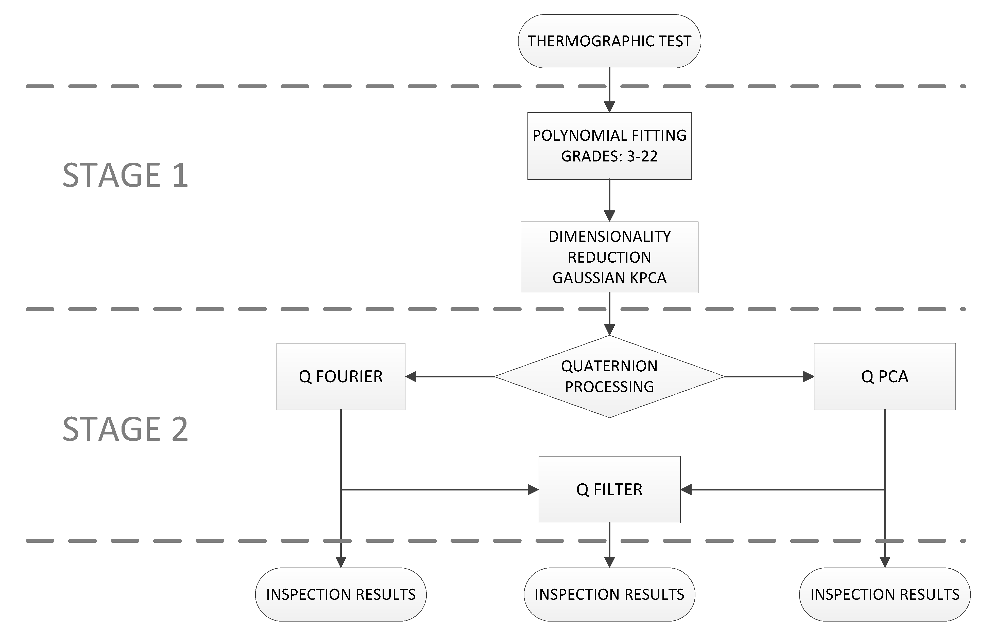
3. Proposed Approach

3.1. Foundation of the Proposed Methodology

The proposed methodology consists of two stages (Figure 1). The first stage applies a novel method called Thermographic Colorization by Computational Synthesis (TCCS), whose main purpose is to extract a large amount of relevant information from NDT thermographic inspections and synthesize it in a single-color video sequence. The hue and saturation characteristics of color images offer greater information synthesis capacity than conventional grayscale images, which capture only information about the intensity levels. The proposed TCCS method synthesizes in only three channels the information contained in a series of thermographic sequences obtained from different polynomial approaches, using dimensionality reduction techniques, so that synthesized information may be represented through color scale images. The second stage of the proposed methodology applies quaternionic algebra operations to the produced color images to optimize the visualization and characterization of the detected defects.
The motivation to develop the TCCS method arises from a limitation detected in TSR and polynomial fitting techniques. These processing techniques approximate the original thermographic signal using a low-degree polynomial, generally between 6 and 8 [23,28], and consider that this unique polynomial represents the best approximation for the thermal evolution of all the observed elements, both defects and internal structure of the material and healthy areas. However, it was verified in previous studies that the degree of the polynomial approximation that produces the highest detection levels is not always the same, and the optimal fitting degree does not guarantee the visualization of all the detected defects [18,21,29]. Furthermore, it was shown in [21] that different degrees of polynomial approximation enable the detection of different defects.

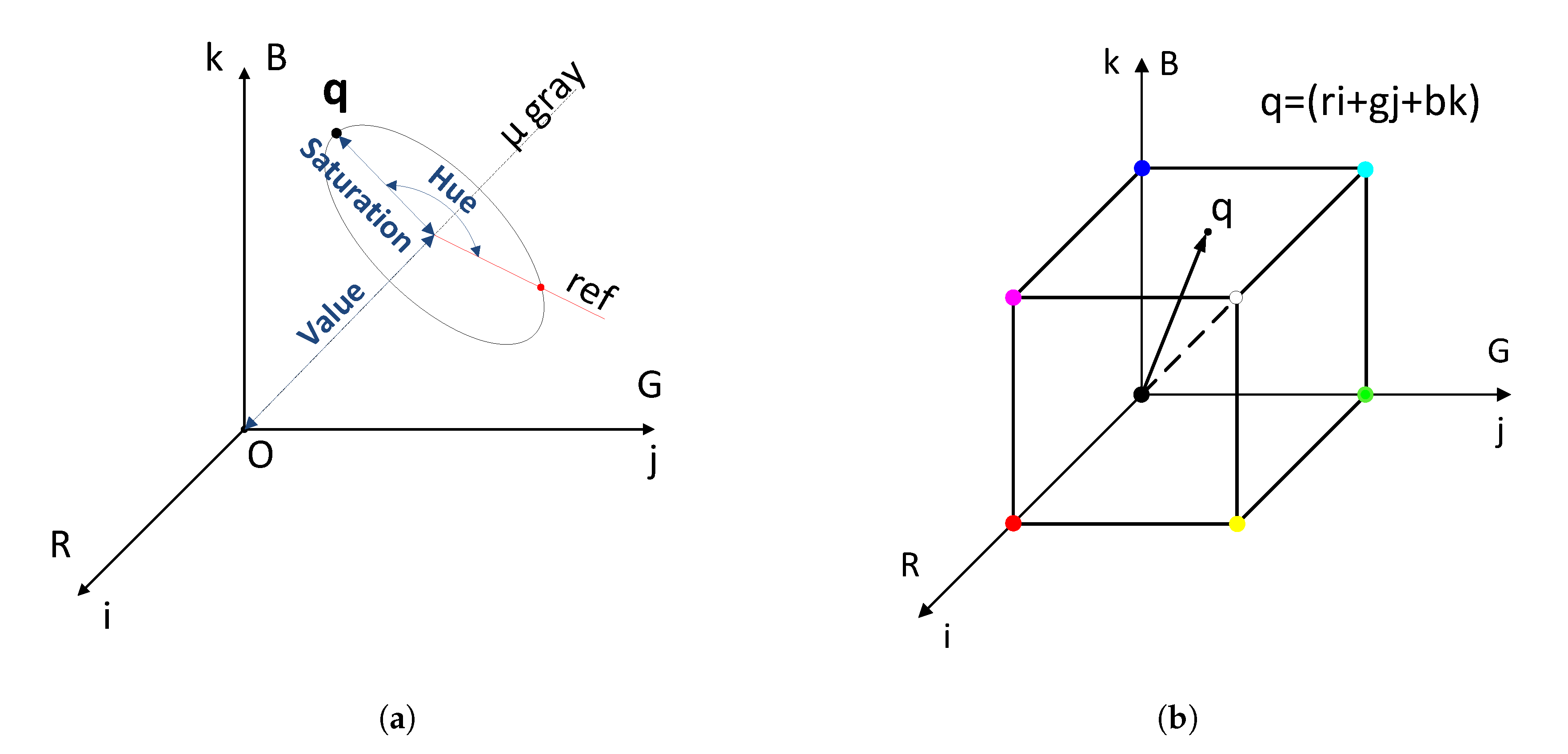
3.2. Description of the Colorization Procedure

The proposed method of thermographic colorization seeks to calculate P polynomials of different degrees for each one that approximate the original thermal sequence. The information contained in these approximations are then synthesized in a reduced number of sequences using dimensionality reduction techniques. In this study, several reduction techniques have been analyzed, including PCA, Kernel principal component analysis (KPCA), independent component analysis (ICA) and minimum noise fraction (MNF).
The dimensionality reduction process is applied to each group of P images that is obtained by selecting the frame in the same position from the P calculated polynomial approximations. This process is carried out for all the frame positions so that a sequence of N color images is available after the reduction procedure, where each color image synthesizes in three channels the information contained in the P approaches initially generated for each frame (Figure 2).
Each of the dimensionality reduction techniques reconstructs the original data in a new space based on a different principle. The PCA and KPCA techniques optimize the variance of the input data, the MNF technique optimizes the SNR and the ICA technique uses the principle of independence (measured by the entropy parameter in this study) to project the original data into the new space. After the application of each of these techniques, a new sequence is obtained with the same number of images as the initial sequence but with new features characteristic of the applied reduction technique.
To complete the proposed colorization process and produce a color image from each frame, three images must be selected from each reconstructed sequence. The most intuitive criterion for selecting the three images with the greatest relevance and informative content is to choose the three images that maximize the dimensional reduction principles applied by each technique, i.e., the variance, the SNR and the entropy. According to this criterion, for the cases of PCA, KPCA and MNF, the first three components are selected, since they are techniques that sort the results in decreasing order of the parameter used, while in the case of ICA, the entropy parameter must be evaluated in the results obtained and then select the three components with higher values, since this technique does not sort the results in the application process.

3.3. Description of the Quaternion Processing

The results obtained after applying the dimensionality reduction techniques are color image sequences, where each color image is made up of a triplet of single-channel images. These single-channel images collect a large amount of information from the original P polynomial approximations based on a reduction technique used in the process. It has been verified in previous studies that, in general, the color images generated from thermographic results lose contrast, and defects that can be seen in the individual channels may be hidden, due to the lower capacity of human vision to perceive variations of certain shades of color than gray scales [21]. On the contrary, human perception is more effective with specific color levels that with intensity gray levels.
Applying image processing to these color images, substantially improves the visualization of the results. Color images can be processed using grayscale imaging techniques applied to each channel individually or specific color imaging techniques applied to the three channels jointly (Figure 3a), but these procedures are sometimes inefficient and unable to perform advanced mathematical operations. Quaternion analysis was used instead in this study to carry out the processing of the color images.
A quaternion q is an element of the 4D normed algebra over R , denoted by H , with the base { 1 , i , j , k } .
H = { q = q 0 1 + q 1 i + q 2 j + q 3 k with q 0 , q 1 , q 2 , q 3 R }
where q 0 , q 1 , q 2 and q 3 are real coefficients, and i, j and k are imaginary operators that satisfy the following multiplication rules:
i 2 = j 2 = k 2 ij = ji = k ki = ik = j jk = kj = i
The components of a pixel in a color image expressed in RGB space can be represented in quaternion form using pure quaternions [30], where the three imaginary parts are used to represent the color components: Red, Green and Blue (Figure 3b). Each pixel at (x,y) coordinates of an RGB image can be expressed as
q ( x , y ) = r ( x , y ) i + g ( x , y ) j + b ( x , y ) k
where r ( x , y ) , g ( x , y ) and b ( x , y ) are the red, green, and blue components, respectively.
Subsequently, color image processing based on quaternion operations is applied, which improves the efficiency of the processing of individual channels and allows operations that cannot be applied to the channels individually or jointly by conventional techniques.
The quaternion analysis techniques that have been applied in this study are Fourier quaternion analysis, quaternion principal component analysis, and quaternion image filtering for color edge detection. Color image filtering has also been applied for smoothing and enhancing, which produces the same results as applying the filtering individually to each channel but improves the efficiency of processing when applied to the three channels at the same time.
Discrete Quaternion Fourier Transform (DQFT)
The definition of Fourier transform has been extended to quaternion analysis based on the operations of multiplication and exponentiation of quaternions [31,32]. As a consequence of the non-commutativity of the quaternion product, there are three different definitions of the discrete quaternion Fourier transform. The expressions for each of the definitions are shown below.
Two-sided DQFT:
F L R ( u , v ) = 1 M N x = 0 M 1 y = 0 N 1 e μ 2 π x u M f ( x , y ) e μ 2 π y v N
Left-sided DQFT:
F L ( u , v ) = 1 M N x = 0 M 1 y = 0 N 1 e μ 2 π x u M + y v N f ( x , y )
Right-sided DQFT:
F R ( u , v ) = 1 M N x = 0 M 1 y = 0 N 1 f ( x , y ) e μ 2 π x u M + y v N
where f is a quaternionic function defined on a set of spatial coordinates ( x , y ) R 2 , F is the DQFT defined over a set of frequency coordinates ( u , v ) R 2 , and μ is a pure unit quaternion that determines a direction in space. It is common in color image processing to choose the direction coinciding with the luminance axis or gray axis. ( r = g = b ).
The results produced by each of the definitions of the DQFT are different. However, for practical NDT visualization and detection purposes, the results of the different transformations are qualitatively similar. In this study, the definition of the left-sided DQFT has been used without loss of generality in the final results.
Quaternion Principal Components Analysis (QPCA)
Quaternion extensions of various classical techniques have been developed, such as principal component analysis, which provide methods for the processing of color images taking into account their particular characteristics through quaternion analysis [33].
There are two different types of eigenvalue problem associated with quaternions due to the non-commutativity of the quaternion product. Given a quaternion matrix M H N × N the left eigenvalues λ l and the right eigenvalues λ r can be determined.
This study has been limited to the problem of right eigenvalues due to theoretical limitations related to left eigenvalues, which do not seem to be fully resolved [34].
Any quaternion matrix M H N × N can be decomposed as
M = W D W *
where W H N × N is a unitary matrix, i.e., W * W = W W * = 1 , containing the eigenvectors of M, and D C N × N is an upper triangular matrix with the diagonal containing the eigenvalues. W * is the quaternion conjugate of W, where given a quaternion q = q 0 1 + q 1 i + q 2 j + q 3 k its quaternion conjugate is q * = q 0 1 q 1 i q 2 j q 3 k . If M is a Hermitian matrix, i.e., M = M * , then its eigenvalues are real ( D R N × N ). Every N × N quaternion matrix has exactly N complex right eigenvalues with non-negative imaginary part, but can have infinite eigenvalues since q 1 λ q is also eigenvalue.
Given a color image of size N × M , represented by a matrix Q H N × M , the quaternion principal component analysis consists of decomposing the mean covariance matrix of a color image C as
C = W D W *
The mean covariance matrix is obtained by the mean value of the covariance matrices calculated for each column q i in the input matrix Q, which is considered the maximum likelihood estimator of the covariance matrices for quaternionic matrices. It can be verified that the matrix C is quaternionic Hermitian and, therefore, the coefficients on the diagonal of D are real values. After diagonalizing the covariance matrix, the new image Y of principal components is obtained by transforming each column of the original image Q to the new base through the expression
y i = W T q i
Quaternion spatial convolution
The spatial convolution technique has also been extended to quaternions, with different definitions because of the non-commutativity of quaternion multiplication. The definition used in this study, widely used in color image processing, indicates that convolution in a quaternionic color image Q H N × M can be expressed as
Q f i l t ( x , y ) = τ 1 = n n τ 2 = m m h l ( τ 1 , τ 2 ) Q ( ( x τ 1 ) ( y τ 2 ) ) h r ( τ 1 , τ 2 )
where h l and h r are two conjugated filters of dimension N × M with N = 2 n + 1 N and M = 2 m + 1 N .
A series of color edge detectors have been developed from this definition of convolution [35]. These methods use two conjugate filters h l and h r that produce a rotation of an angle π around the gray axis at each pixel and compare its value with neighboring pixels.
The edge detection filter used in this study, composed of a pair of conjugate filters, is defined as follows:
h l = 1 1 1 0 0 0 q q q a n d h r = 1 1 1 0 0 0 q * q * q *
where the q value is calculated as q = e μ π 2 , being μ = μ g r i s = i + j + k 3 the grayscale axis.

3.4. Description of the Evaluation Metrics

The quality of the signals generated, processed or measured is a fundamental requirement in all engineering disciplines. Engineers and researchers characterize signals quantitatively to assess the quality of equipment and processes, and to act accordingly. For this purpose, a large number of signal quality metrics have been developed [36,37].
To control the quality of the images and to be able to maintain it, and even improve it, it is necessary to measure the quality in each of the stages they go through. Presently, Image Quality Assessment (IQA) is of great importance in visual communication and is essential for most image processing applications.
In general, image quality metrics can be classified into subjective and objective. Subjective metrics present important practical limitations, mainly due to the high degree of variability of the response to certain factors. Among the different options available in objective evaluation, there are scalar metrics, which include bivariate measures such as the mean square error and the L p norm, metrics that try to imitate the human visual system such as the Human Visual System (HVS), and also graphic metrics. Within objective evaluation, pixel-based techniques, such as Mean Square Error (MSE), Root Mean Square Error (RMSE), and signal-to-noise ratio (SNR), are widely applied due to its simple calculation methodology. In general, these metrics are defined only for monochromatic images, discarding information related to color.
The physical meaning of the SNR metric depends on the magnitudes involved. The general purpose of the SNR is to compare the level of a desired signal to the level of the background noise, and is often calculated in decibel scales for magnitudes with wide dynamic range [13,38]. The following definitions for SNR have been used in this study to evaluate the performance of the proposed analysis methodology and compare it to conventional processing algorithms [13]:
S N R 1 = μ S σ N
S N R 2 = μ S μ N σ N
S N R 3 = 10 log 10 μ S μ N 2 σ N 2
S N R 4 = σ S σ N
S N R 5 = σ S 2 σ N 2
S N R 6 = 10 log 10 σ S 2 σ N 2
S N R 7 = μ S μ N ( σ S 2 + σ N 2 ) / 2
where σ S is the standard deviation of the signal in the defect region of the image, σ N is the standard deviation of the noise in the reference or sound region of the image, μ N is the mean level of the noise in the reference or sound region of the image and μ S is the mean level of the signal in the defect region of the image.

4. Results

4.1. Data Used in the Evaluation

Computationally generated thermal data has been used in the first analysis stage of this study, in order to avoid the influence of imperfections inherent to real situations on the behavior of the analyzed methods. The absence of effects related to the noise produced by the IR sensor, the heterogeneities of the stimulation on the surface of the inspected objects and the uncertainties about the characteristics of the base material and the defects, enables the analysis of the fundamental characteristics of the developed methods and to determine their characterization capabilities.
The generation of synthetic data has been carried out by simulating an ideal thermographic NDT test. The equation that governs the heat transfer process conducted in NDT thermographic inspections has been defined by means of a heterogeneous 3D isotropic thermal diffusion model and the consideration of a series of simplifying hypotheses, such as opaque, heterogeneous and isotropic material, with thermophysical properties independent of temperature, no internal heat sources, and incident energy being diffuse and homogeneously distributed along the external surface. This model is mathematically represented by Equation (24).
T ( x , t ) t · ( α ( x ) T ( x , t ) ) = F ( x , t )
x R 3 , t 0 , α ( x ) R +
where T is the temperature at each material point, α is the thermal diffusivity of the material α = k / ( ρ c p ) , k is the thermal conductivity, ρ is the density of the material, c p is the specific heat at constant pressure and F represents the heat sources. The Equation (24) states the balance among the heat generated inside the material ( F ( x , t ) ), the net heat flux in the material ( ρ ( x ) c p ( x ) T ( x , t ) / t ) and the heat stored inside the material ( · ( k ( x ) T ( x , t ) ) ).
The type of material modeled consisted of a Carbon Fiber Reinforced Polymer (CFRP). This is a composite material with excellent mechanical properties and relationship between resistance and weight, widely used in the aeronautical industry. The sample consisted of several layers with the fibers oriented in a specific direction, stacked and bonded by an epoxy resin. The thermal characteristics of this material were modeled by three different values of thermal diffusivity, one for each coordinate axis. These diffusivity values have been estimated as the mean value of the data obtained from various bibliographic sources [39,40], so that the values finally used have been α x = 7.0 ± 2 · 10 7   m 2 / s , α y = 3.5 ± 2 · 10 7   m 2 / s and α z = 1.0 ± 0.3 · 10 6   m 2 / s . This sample was designed with 18 internal defects of sizes 10 × 10 mm 2 and 5 × 5 mm 2 located at different depths from 1 mm to 9 mm (Figure 4a). These defects were modeled with thermal properties simulating delaminations with α = 1.25 ± 2 · 10 7   m 2 / s . This diffusivity value corresponds to Polytetrafluoroethylene (PTFE), whose use to simulate delaminations is widespread.
Optical Step Heating Thermography (OSHT) has been modeled for experimental capacity reasons. The stimulation conditions simulated a constant heating of the inspected sample, applied to its external surface by means of halogen lamps, generating a heat flow into the material (Figure 4b). The thermal stimulation has been applied for 10 s, homogeneously distributed over the entire external surface with an energy of F = 1.5 K/s. This value was previously estimated experimentally through laboratory tests.
The spatial and temporal evolution of temperature has been calculated from (24) by programming an algorithm for numerical resolution by finite differences and considering representative parameters of NDT thermographic inspections and the inspected material (Figure 4c). The theoretical thermal evolution was corrupted with noise to obtain data closer to real conditions. It was demonstrated in previous studies that the noise affecting IR sensors can be modeled by Gaussian white noise [41,42], so this was the type of noise used to approximate the theoretical data to actual experimental situations (Figure 4d).
The next stage in the analysis of the proposed methods has been carried out by using data collected from experimental tests performed in the laboratory. OSHT inspections have been conducted using two 1000 W halogen lamps at 80% of their capacity. The lamps heated the material under inspection for 10 s and both the heating and the cooling phases were recorded, making a total inspection time of 20 s. Infrared images have been acquired with a FLIR SC5500 model and a front face test setup (Figure 5a). A slight deviation was applied in the perpendicular orientation of the camera with respect to the inspected sample to avoid reflections of the sensor itself on the surface of the material. The sample used in the experimental analysis was made in a sandwich structure of composite material with 1 mm thick skins and 5 mm thick foam core. The defects intentionally introduced in this sample were small sheets of PTFE of sizes 10 × 10 mm 2 , 5 × 5 mm 2 , 5 × 3 mm 2 and 3 × 3 mm 2 . The defects were located at two different depths, under 1 mm skin and under 1 mm skin and additional 0.1 mm adhesive layer (Figure 5b). For repeatability analysis, two defects of each size were set at each depth. The emissivity of this sample was estimated experimentally as 0.91.

4.2. Results in the Colorization Procedure

The first stage in the evaluation of the proposed colorization techniques has consisted of calculating the polynomial approximations of the original sequence of computationally generated data. A total of 20 polynomial approximations have been calculated for degrees 3 to 22. No approximations of a degree lower than 3 have been calculated due to the high inaccuracy of the approximation obtained, nor have approximations been calculated for degrees greater than 22 because they do not provide additional information regarding approximations of lower degrees.
After calculating the approximation data, dimensionality reduction techniques have been applied to the generated sequence to obtain a new sequence of color images with synthesized information. Finally, Quaternion Fourier Transformation (QFT) and Quaternion Principal Component Analysis have been applied to the synthesized sequences, and the resulting images have been processed by quaternionic filtering to optimize the visualization of the detections.
Several reduction techniques have been analyzed, including PCA, KPCA, ICA and MNF. The parameters used for PCA and MNF are defined by the mathematical method itself. On the other hand, the kurtosis metric has been used in the ICA analysis, and kernels with standard deviation values of 0.01, 0.05, 0.1, 0.5, 1 and 5 have been used in the Gaussian KPCA. The computational algorithms for the application of these reduction methods have been programmed in MATLAB with the support of the hyperspectral analysis package [43].
The different techniques have been applied to the original sequence of synthetic data, obtaining the corresponding processed sequences. It was found that the reduction technique that produced the best results, being able to synthesize the greatest amount of relevant information in 3 images, was the KPCA technique, followed by the MNF, PCA and ICA technique, respectively. Some representative results obtained with the different colorization techniques are shown in Figure 6.
In general, and as can be seen in Figure 6, the results provided by the ICA and PCA reduction techniques produce a visualization of different defects using different color ranges, but on the contrary, these two techniques collect large amount of noise in the results, hiding defects that are visible by other reduction techniques (Figure 6a,b). The MNF technique significantly filters the noise level of the images; however, this filtering is produced at the expense of an important reduction in the signal value of defects, obtaining reduced detection levels (Figure 6c). Finally, the KPCA technique produces satisfactory results not only by reducing the noise level of the image but also by increasing the flaw detection capacity (Figure 6d).
The reduction technique that produced the best results in terms of reducing noise levels and improving defect detection levels was the KPCA. For this reason, it has been chosen as the reduction technique to be applied for dimensionality reduction before the quaternionic processing.

4.3. Results in the Quaternion Processing

The results obtained after the dimensionality reduction process applied to the sequence of polynomial approximations have been processed with Quaternion Fourier Transform and Quaternion Principal Component Analysis. Subsequently, the results obtained with the application of QFT and QPCA have been processed using quaternionic filtering to optimize the visualization. The quaternionic processing algorithms have been programmed in MATLAB with the additional support of the quaternion package [44]. Some of the results obtained for each of the quaternionic processing techniques are shown below.
Quaternion Fourier analysis requires a quaternion to which apply the processing and, in addition, it also requires a unit quaternion that defines an analysis direction. Depending on the analysis direction, the QFT result varies. Without going into theoretical details about the effect of the analysis direction, which is beyond the scope of the current study, an experimental analysis of the effect it produces on the visualization of defects has been carried out. For this purpose, 32 different directions defined by the radii of a unit sphere have been analyzed, as shown in Figure 7a.
The values required for the calculation of the evaluation metrics, i.e., the mean values and standard deviations of the areas occupied by the defects and the healthy reference areas close to them, are extracted from the results obtained with the QFT processing. These values are calculated for each of the existing defects and for each of the 3 color channels defined by the quaternion axes. An efficient way to collect these data has consisted of storing them using analysis directions spheres, where the calculated values are stored as color data expressed in RGB space for each of the analyzed directions (Figure 7b). This way, each point of the resulting sphere indicates the QFT analysis direction by its spatial coordinates, and the corresponding calculated values for the metrics by its RGB color.
After the application of the QFT processing with the direction analysis to the different reduced sequences, the data measured for each defect are recovered and the metrics are calculated. The results obtained in the calculation of the metrics can be analyzed graphically through spheres of directions where the radius of the sphere at each point coincides with the value of the metric calculated for each analysis direction defined by the point, being the optimal direction the one with a larger radius (Figure 7c).
Figure 8 shows some representative results obtained with the QFT technique. It was observed that the defects that are detected are represented in different color depending on the depth. Defects of the same type located at different depths produce different color tones, while defects of the same type located at the same depth produce similar tones. This behavior is observed in the results obtained with the synthetic data, where the induced defects are of the same type and are located at different depths (Figure 8a–c, and with the experimental specimen, which contains defects of the same type and located at the same depth but of different sizes (Figure 8d–f). Frequently, the QFT results that produce the highest levels of defect detection are in the first 10% of the results in the generated sequence. However, numerous cases have been found in which this rule is not followed.
The application of QPCA processing requires only the quaternion being processed. In Figure 9 some results obtained from the application of QPCA to the sequence reduced by Gaussian KPCA are shown. Generally, the results that produce the highest levels of detection are the frames included within the first 5 results of the processed sequence, increasing the noise level and losing detection capacity for frames with further positions. Results with lower noise levels lose the ability to detect most subtle defects. The results that allow the detection of a greater number of defects, located deeper, also contain a certain level of noise, so that in general the optimal detections do not occur in the first result. As with QFT processing, QPCA results generate similar color tones for defects of the same type and located at the same depth (Figure 9a–c), while defects located at different depths generate different color tones (Figure 9d–f).
Finally, quaternionic filtering by spatial convolution (QFILT) has been applied to the results obtained with the application of QFT and QPCA. The objective of this processing is to enhance the edges of the defects to improve the visualization and facilitate their location. For its application, the pair of conjugate filters defined in the Quaternion Spatial Convolution section together with a scale factor S = 1 / 6 has been used to average the sum of the 6 pixel values defined by the pair of filters. Some results obtained in this analysis are shown in Figure 10, where the upper row corresponds to the starting results obtained with QFT and QPCA, and the lower row corresponds to the results obtained after the quaternionic filtering. It is observed that the edges of the defects appear colored with different shades depending on the original color of the defect, while the internal areas appear with colors tending to shades of gray. Additionally, the edges of the defects are not shown with a single color but are represented with two different tones. This effect occurs as a result of the path followed in the convolution process. In this study, the path followed in the convolution went from top to bottom and from left to right. The change of the path produces different tones at the edges.

5. Discussion

The results obtained with the proposed colorization methodology have been compared with conventional processing techniques, including the original sequence of thermographic data, the approximate polynomial sequences and their first two derivatives, as well as the principal component analysis applied to the original sequence. The metrics used to evaluate the quality of the results produced have been the SNR in the different versions described before. The SNR calculation procedure was automated, taking advantage of the prior knowledge of the position of the defects, locating the measurement areas of the defects and their corresponding healthy reference areas for each of the induced faults.
To correctly compare data of different nature, such as the grayscale images of the original sequence and conventional processes, and the color images of the sequences resulting from the colorization processing, the definition for the SNR has been generalized. The magnitude used to calculate these metrics in grayscale images is the intensity or luminance of the image. In the case of color images represented in RGB space, this magnitude or similar does not exist, but the RGB components are available, which do not describe image intensity properties. To be able to compare color images with grayscale images, it is necessary to represent the color images in a space that separates the intensity characteristics from the characteristics exclusive to the color.
Colors can be represented in the HSV space so that the value (V), hue (H) and saturation (S) of each pixel in the image are available [45]. The value component is naturally comparable to the intensity of grayscale images, while the other two components provide additional information unique to color images. Intuitively, it is reasonable to think that a color image provides more information than a grayscale image as it has two additional information channels. In this sense,
The saturation component provides extra information about the intensity of the color, which could be related to the severity of a defect. However, the hue component is a magnitude that does not have a defined order, so the hue value does not provide useful information on the quality of defect detection as it cannot be compared in an orderly manner. Due to this limitation, it was decided to discard this color space to evaluate the results obtained in the colorization techniques. The color space that was finally used was the Lab space [46,47].
The Lab color space (L*a*b* or CIELAB) is the color model normally used to describe all the colors that the human eye can perceive (Figure 11). It was developed specifically for this purpose by the Commission Internationale d’Eclairage (International Commission on Illumination). The goal of the Lab space is to produce a color space that is more “perceptually linear” than other color spaces, i.e., a change of the same amount in any color value produces a visual change of the same intensity. Due to the property of perceptual linearity of the Lab space, these parameters make it possible to quantify color variations and relate them to flaw detection levels.
The procedure followed to evaluate the results obtained consisted of transforming the RGB color values (Figure 11a), obtained by means of colorization and quaternionic processing techniques, to the Lab color space (Figure 11b). Next, the mean values and variances of the measurement areas of each defect are calculated for each of the Lab components ( μ L , μ a , μ b , σ L , σ a and σ b ,), and then the magnitude of the vector defined by these components is calculated through the expressions (25) and (26). Finally, the formulas of the SNR metrics are applied with the obtained values μ q and σ q .
μ q = μ L 2 + μ a 2 + μ b 2
σ q = σ L 2 + σ a 2 + σ b 2

Analysis of the Results and Comparison to Common Processing Techniques

In this study, a large amount of data has been generated as a result of the analysis of different dimensionality reduction techniques, different quaternionic data processing techniques and the application of different SNR metrics on a total of 34 defects. The presentation and discussion of the results has been simplified to show those of greater relevance. For this, the results obtained for the dimensionality reduction techniques using Gaussian KPCA are presented below, with the QFT, QPCA and quaternionic filtering by spatial convolution (QFILT) processing, and the seven different SNR metrics calculated for the synthetic defects located under 1 mm (def1), 3 mm (def2) and 5 mm (def3), and the experimental defects located deeper and with larger size (def4), medium size (def5) and smaller size (def6).
Figure 12 shows the graphical representation by bar diagrams of the maximum SNR values obtained for the defects analyzed with the different quaternionic processing techniques together with the values obtained with conventional thermographic data processing techniques (polynomial fitting, first and second derivatives, and PCA) as well as the value obtained with the original sequence. The y-axis values are represented in a logarithmic scale to correctly visualize the data for all cases. The SNR values have been calculated for the intensity data considering them as gray colors, i.e., assigning the 3 color components the same value, equal to the value of its intensity, and applying the same procedure as for the color data produced in the quaternionic processing.
It can be observed in Figure 12 that the ranges of the values obtained for the different cases of SNR are very different, which means that different definitions of SNR are not mutually comparable. In most cases, larger and more superficial defects produce higher SNR values. It can be verified that quaternionic processing techniques produce higher SNR values than conventional ones for all the SNR cases except for SNR7, where the experimental defects produce maximum values for first derivative and conventional PCA. QFT processing has provided maximum SNR values for all the synthetic defect cases, while QPCA has provided maximum SNR values for the experimental defects. In general, the QFILT processing does not increase the SNR with respect to QFT and QPCA, what can be justified by the effect that this processing produces to the input data. The area inside the defects acquires a homogeneous shade tending to gray, while the edges are highlighted with colors. Most probably the use of another sharpness-type metric provided a more favorable evaluation for this quaternionic processing.
Figure 13 shows the maximum SNR values obtained for the analyzed defects by applying quaternionic processing to the different cases of dimensionality reduction by Gaussian KPCA. The y-axis values are represented in a logarithmic scale to correctly visualize the data for all cases. It is verified again that the ranges of values obtained for the different cases of SNR are very different, which means that different definitions of SNR are not mutually comparable.
It is observed that the maximum values of SNR are produced for different values of variance depending on the defects analyzed and the metric used. For SNR1, the maximum values for synthetic defects are obtained with variances greater than 0.05, while for experimental defects they are obtained for variances greater than 0.1. In both cases the variance of 0.01 obtained acceptable results. For SNR2, the maximum values are produced for a variance of 0.05 in the case of experimental defects, while for synthetic defects, variances greater than 0.05 maximize defects located at a depth less than or equal to 3 mm and a variance of 0.01 maximizes the deeper defects. SNR3 produces results similar to SNR2 in the case of synthetic defects, while for experimental defects, very similar results are obtained for all the analyzed variances, with slightly higher values for variances less than 0.5. For SNR4 and SNR5, synthetic defects located at depths less than or equal to 3 mm produce maximum values for variances greater than 0.05, while defects located at greater depths maximize SNR for variances less than 0.05. Regarding the experimental defects, the SNR values are maximized for variances less than 0.5 in both cases. SNR6 produces responses similar to SNR4 and SNR5 for the case of synthetic defects, while for experimental defects it produces very similar results for all the variance values analyzed, with slightly higher levels for variances of 0.05 and 0.1. Finally, for SNR7, synthetic defects located at depths greater than 3 mm produce maximum values for variances greater than 0.5, while defects at depths less than or equal to 3 mm maximize the SNR for variances less than 1. Regarding the experimental defects, in all cases the maximum values of SNR occur for variances greater than 0.01.
Figure 14 shows the mean SNR values obtained with the defects analyzed for each of the SNR metric definitions. The y-axis values are represented in a logarithmic scale to be able to correctly visualize the data for all cases. Important differences are observed among the values that each of the definitions produces. In general, defects located at shallower depths and larger defects have produced higher SNR values for all metrics except for SNR1, where synthetic defects at different depths have very similar values, even in some cases, defects located at greater depths have higher SNR values.
It is observed in Figure 14 that the SNR5 metric produces very high values, of the order of 10 6 , for the most superficial synthetic defects, compared to the rest of the synthetic and experimental defects of the order of 10 2 . The values produced by SNR3 and SNR6 for the different defects are much more balanced than the rest of the metrics, due to the application of logarithms in their calculation. For the rest of the metrics, the differences between the SNR values for different defects is much more significant, clearly highlighting the values for the most superficial synthetic defects.

6. Conclusions

In this study, a new methodology for the processing and analysis of NDT thermographic sequences is proposed. This methodology consists of two stages. The first stage applies a novel method called Thermographic Colorization by Computational Synthesis (TCCS), which extracts a large amount of relevant information from NDT thermographic inspections and synthesize it in a single-color video sequence. The second stage applies quaternionic algebra operations to the produced color images to optimize the visualization and characterization of the detected defects.
The information synthesis process is carried out by means of dimensionality reduction techniques. In this study, four reduction techniques have been analyzed: Independent Component Analysis, Principal Component Analysis, Kernel Principal Component Analysis and Minimum Noise Fraction, proving that the KPCA technique produces the best results. After the data synthesis colorization stage, color image processing techniques based on quaternion algebra operations are applied. Three different techniques of quaternion analysis have been applied: Quaternion Fourier transform, Quaternionic Principal Components Analysis and Quaternionic Filtering by Spatial Convolution.
A graphical method for optimizing the analysis directions in QFT has been developed that enables the automatization of this quaternionic processing. This method is based on the use of spheres to define the directions of analysis, synthesize the information about the output signal levels through the color of each point on the sphere, and graphically represent the final results produced by the assessment metrics.
The use of color images as results of NDT thermographic inspections makes the conventional SNR definitions used to assess the results not directly applicable. In order to assess results represented by color images and compare them with conventional results represented by grayscale images, the application method of SNR metrics has been generalized in this study. For this, a perceptually linear color space (Lab) has been used, to which the color and gray data are transformed, and the definition of SNR has been adapted to extend it to the 3D case.
The evaluation of the results obtained has shown that the proposed methodology improves the results compared to conventional thermographic NDT processing, increasing the level of detection and improving the distinction of the defects by their representation in different color shades. The results have been evaluated with different definitions of SNR, for most of which the quaternionic Fourier and principal component analyses produce a high increase in the SNR level. It has been found that quaternionic filtering by spatial convolution does not produce an increase in SNR, even though it improves the visualization of the detected defects and facilitates their characterization. This shows that the SNR metric is not suitable for evaluating processing results whose effect is focused on edge enhancement.
Finally, the analysis of the results obtained using different SNR metrics has demonstrated that the choice of the SNR definition to assess the results has a great impact in the final values, and it can be concluded that the values obtained with different SNR definitions are not comparable among them, producing values of very different orders of magnitude for the same defect.

Author Contributions

Conceptualization, P.V., R.U. and J.P.; methodology, P.V. and I.S.d.O.; software, P.V. and R.U.; validation, P.V., R.U. and J.P.; formal analysis, P.V.; investigation, P.V.; resources, R.U., J.P. and I.S.d.O.; data curation, P.V. and I.S.d.O.; writing—original draft preparation, P.V.; writing—review and editing, P.V., R.U. and J.P.; visualization, I.S.d.O.; supervision, R.U., J.P. and I.S.d.O.; project administration, P.V. All authors have read and agreed to the published version of the manuscript.

Funding

This research received no external funding.

Conflicts of Interest

The authors declare no conflict of interest.

References

  1. Maldague, X. Nondestructive Evaluation of Materials by Infrared Thermography; Springer Science & Business Media: Berlin/Heidelberg, Germany, 2012. [Google Scholar]
  2. Usamentiaga, R.; Venegas, P.; Guerediaga, J.; Vega, L.; Molleda, J.; Bulnes, F. Infrared thermography for temperature measurement and non-destructive testing. Sensors 2014, 14, 12305–12348. [Google Scholar] [CrossRef] [PubMed] [Green Version]
  3. Tomlinson, C.; Chapman, L.; Thornes, J.; Baker, C. Remote sensing land surface temperature for meteorology and climatology: A review. Meteorol. Appl. 2011, 18, 296–306. [Google Scholar] [CrossRef] [Green Version]
  4. Lahiri, B.; Bagavathiappan, S.; Jayakumar, T.; Philip, J. Medical applications of infrared thermography: A review. Infrared Phys. Technol. 2012, 55, 221–235. [Google Scholar] [CrossRef] [PubMed]
  5. Kylili, A.; Fokaides, P.; Christou, P.; Kalogirou, S. Infrared thermography (IRT) applications for building diagnostics: A review. Appl. Energy 2014, 134, 531–549. [Google Scholar] [CrossRef]
  6. Lim, G.; Bae, D.; Kim, J. Fault diagnosis of rotating machine by thermography method on support vector machine. J. Mech. Sci. Technol. 2014, 28, 2947–2952. [Google Scholar] [CrossRef]
  7. Herschel, W., XV. Experiments on the solar, and on the terrestrial rays that occasion heat; with a comparative view of the laws to which light and heat, or rather the rays which occasion them, are subject, in order to determine whether they are the same, or different. Philos. Trans. R. Soc. Lond. 1800, 90, 293–326. [Google Scholar]
  8. Pergande, D.; Geppert, T.M.; Rhein, A.V.; Schweizer, S.L.; Wehrspohn, R.B.; Moretton, S.; Lambrecht, A. Miniature infrared gas sensors using photonic crystals. J. Appl. Phys. 2011, 109, 083117. [Google Scholar] [CrossRef]
  9. Keränen, K.; Mäkinen, J.T.; Korhonen, P.; Juntunen, E.; Heikkinen, V.; Mäkelä, J. Infrared temperature sensor system for mobile devices. Sens. Actuators A Phys. 2010, 158, 161–167. [Google Scholar] [CrossRef]
  10. Khodayar, F.; Sojasi, S.; Maldague, X. Infrared thermography and NDT: 2050 horizon. Quant. InfraRed Thermogr. J. 2016, 13, 210–231. [Google Scholar]
  11. Beemer, M.F.; Shepard, S.M. Aspect ratio considerations for flat bottom hole defects in active thermography. Quant. InfraRed Thermogr. J. 2018, 15, 1–16. [Google Scholar] [CrossRef]
  12. Mendioroz, A.; Fuggiano, L.; Venegas, P.; Ocáriz, I.S.d.; Galietti, U.; Salazar, A. Characterizing Subsurface Rectangular Tilted Heat Sources Using Inductive Thermography. Appl. Sci. 2020, 10, 5444. [Google Scholar] [CrossRef]
  13. Usamentiaga, R.; Ibarra-Castanedo, C.; Maldague, X. More than fifty shades of grey: Quantitative characterization of defects and interpretation using snr and cnr. J. Nondestruct. Eval. 2018, 37, 25. [Google Scholar] [CrossRef]
  14. Švantner, M.; Muzika, L.; Chmelík, T.; Skála, J. Quantitative evaluation of active thermography using contrast-to-noise ratio. Appl. Opt. 2018, 57, D49–D55. [Google Scholar] [CrossRef] [PubMed]
  15. Jaffery, Z.A.; Dubey, A.K. Design of early fault detection technique for electrical assets using infrared thermograms. Int. J. Electr. Power Energy Syst. 2014, 63, 753–759. [Google Scholar] [CrossRef]
  16. Dutta, T.; Sil, J.; Chottopadhyay, P. Condition monitoring of electrical equipment using thermal image processing. In Proceedings of the 2016 IEEE First International Conference on Control, Measurement and Instrumentation (CMI), Kolkata, India, 8–10 January 2016; pp. 311–315. [Google Scholar]
  17. Al-Musawi, A.K.; Anayi, F.; Packianather, M. Three-phase induction motor fault detection based on thermal image segmentation. Infrared Phys. Technol. 2020, 104, 103140. [Google Scholar] [CrossRef]
  18. Roche, J.; Leroy, F.; Balageas, D. Images of thermographic signal reconstruction coefficients: A simple way for rapid and efficient detection of discontinuities. Mater. Eval. 2014, 72, 73–82. [Google Scholar]
  19. Roche, J.; Balageas, D. Detection and characterization of composite real-life damage by the TSR-polynomial coefficients RGB-projection technique. In Proceedings of the 12th International Conference on Quantitative Infrared Thermography (QIRT 2014), Bordeaux, France, 7–11 July 2014; pp. 1–10. [Google Scholar]
  20. Balageas, D.L.; Roche, J.M.; Leroy, F.H.; Liu, W.M.; Gorbach, A.M. The thermographic signal reconstruction method: A powerful tool for the enhancement of transient thermographic images. Biocybern. Biomed. Eng. 2015, 35, 1–9. [Google Scholar] [CrossRef] [Green Version]
  21. Venegas, P.; Usamentiaga, R.; Perán, J.; Sáez de Ocáriz, I. Advances in RGB Projection Technique for Thermographic NDT: Channels Selection Criteria and Visualization Improvement. Int. J. Thermophys. 2018, 39, 95. [Google Scholar] [CrossRef]
  22. Shepard, S.M.; Lhota, J.R.; Rubadeux, B.A.; Wang, D.; Ahmed, T. Reconstruction and enhancement of active thermographic image sequences. Opt. Eng. 2003, 42, 1337–1343. [Google Scholar] [CrossRef]
  23. Shepard, S. System for Generating Thermographic Images Using Thermographic Signal Reconstruction. U.S. Patent 6,751,342, 15 June 2004. [Google Scholar]
  24. Maldague, X.; Galmiche, F.; Ziadi, A. Advances in pulsed phase thermography. Infrared Phys. Technol. 2002, 43, 175–181. [Google Scholar] [CrossRef] [Green Version]
  25. Rajic, N. Principal component thermography for flaw contrast enhancement and flaw depth characterisation in composite structures. Compos. Struct. 2002, 58, 521–528. [Google Scholar] [CrossRef]
  26. Lopez, F.; Ibarra-Castanedo, C.; de Paulo Nicolau, V.; Maldague, X. Optimization of pulsed thermography inspection by partial least-squares regression. NDT E Int. 2014, 66, 128–138. [Google Scholar] [CrossRef]
  27. Madruga, F.J.; Ibarra-Castanedo, C.; Conde, O.M.; López-Higuera, J.M.; Maldague, X. Infrared thermography processing based on higher-order statistics. NDT E Int. 2010, 43, 661–666. [Google Scholar] [CrossRef]
  28. Shepard, S. Temporal Noise Reduction, Compression and Analysis of Thermographic Image Data Sequences. U.S. Patent 6,516,084, 4 February 2003. [Google Scholar]
  29. Roche, J.; Leroy, F.; Balageas, D. Information condensation in defect detection using TSR coefficients images. In Proceedings of the 12th International Conference on Quantitative Infrared Thermography (QIRT 2014), Bordeaux, France, 7–11 July 2014. [Google Scholar]
  30. Sangwine, S. Fourier transforms of colour images using quaternion or hypercomplex, numbers. Electron. Lett. 1996, 32, 1979–1980. [Google Scholar] [CrossRef]
  31. Ell, T.; Sangwine, S. Hypercomplex Fourier transforms of color images. IEEE Trans. Image Process. 2007, 16, 22–35. [Google Scholar] [CrossRef]
  32. Dubey, V. Quaternion Fourier transform for colour images. Int. J. Comput. Sci. Inf. Technol. 2014, 5, 4411–4416. [Google Scholar]
  33. Chang, J.; Ding, J. Quaternion matrix singular value decomposition and its applications for color image processing. In Proceedings of the International Conference on Image Processing, Barcelona, Spain, 14–18 September 2003; Volume 1, pp. 805–808. [Google Scholar]
  34. Huang, L.; So, W. On left eigenvalues of a quaternionic matrix. Linear Algebra Appl. 2001, 323, 105–116. [Google Scholar] [CrossRef] [Green Version]
  35. Denis, P.; Carre, P.; Fernandez-Maloigne, C. Spatial and spectral quaternionic approaches for colour images. Comput. Vis. Image Underst. 2007, 107, 74–87. [Google Scholar] [CrossRef] [Green Version]
  36. Wang, Z.; Bovik, A.; Sheikh, H.; Simoncelli, E. Image quality assessment: From error visibility to structural similarity. IEEE Trans. Image Process. 2004, 13, 600–612. [Google Scholar] [CrossRef] [Green Version]
  37. Hu, Y.; Loizou, P. Evaluation of objective quality measures for speech enhancement. IEEE Trans. Audio Speech Lang. Process. 2008, 16, 229–238. [Google Scholar] [CrossRef]
  38. Smith, S. Digital Signal Processing: A Practical Guide for Engineers and Scientists; Elsevier: Amsterdam, The Netherlands, 2013. [Google Scholar]
  39. Battaglia, J.; Saboul, M.; Pailhes, J.; Saci, A.; Kusiak, A.; Fudym, O. Carbon epoxy composites thermal conductivity at 77 K and 300 K. J. Appl. Phys. 2014, 115, 223516-1–223516-4. [Google Scholar] [CrossRef] [Green Version]
  40. Joven, R.; Das, R.; Ahmed, A.; Roozbehjavan, P.; Minaie, B. Thermal properties of carbon fiber/epoxy composites with different fabric weaves. In Proceedings of the SAMPE International Symposium Proceedings, Society for the Advancement of Material and Process Engineering, Charleston, SC, USA, 22–25 October 2012. [Google Scholar]
  41. Li, N.; Huai, W.; Wang, S.; Ren, L. A real-time infrared imaging simulation method with physical effects modeling of infrared sensors. Infrared Phys. Technol. 2016, 78, 45–57. [Google Scholar] [CrossRef]
  42. Rogalski, A. Recent progress in infrared detector technologies. Infrared Phys. Technol. 2011, 54, 136–154. [Google Scholar] [CrossRef]
  43. Gerg, I. MATLAB Hyperspectral Toolbox, 2008–2012. Available online: https://github.com/isaacgerg/matlabHyperspectralToolbox (accessed on 12 January 2021).
  44. Sangwine, S.J.; Bihan, N.L. The Quaternion Toolbox for MATLAB, 2008–2017. Available online: http://qtfm.sourceforge.net/ (accessed on 12 January 2021).
  45. Ibraheem, N.A.; Hasan, M.M.; Khan, R.Z.; Mishra, P.K. Understanding color models: A review. ARPN J. Sci. Technol. 2012, 2, 265–275. [Google Scholar]
  46. Schanda, J. Colorimetry: Understanding the CIE System; John Wiley & Sons: Hoboken, NJ, USA, 2007. [Google Scholar]
  47. Fairchild, M. Color Appearance Models; John Wiley & Sons: Hoboken, NJ, USA, 2013. [Google Scholar]
Figure 1. Methodology followed in the proposed quaternionic NDT thermography.
Applsci 11 00790 g001
Figure 2. Dimension reduction scheme applied with the proposed colorization method.
Applsci 11 00790 g002
Figure 3. Color image processing: (a) quaternionic relationships between RGB and HSV color spaces, (b) geometric representation of a color by quaternions.
Applsci 11 00790 g003
Figure 4. Modeled NDT thermographic inspections: (a) position of defects with depth indicated numerically [mm], (b) thermal stimulation considered in the model, (c) scaled temperature values obtained with the theoretical model in absence of noise after 5 s in the heating process, (d) scaled temperature values obtained with the theoretical model in the presence of noise after 5 s in the heating process.
Applsci 11 00790 g004
Figure 5. Experimental NDT thermographic inspections: (a) setup of the laboratory tests, (b) depth of defects in the inspected material.
Applsci 11 00790 g005
Figure 6. RGB images obtained by the projection of the results produced with the different dimensionality reduction techniques at the instant 5 s in the thermal sequence: (a) ICA, (b) PCA, (c) MNF, (d) KPCA.
Applsci 11 00790 g006
Figure 7. Supporting spheres used in the optimization of the analysis directions in QFT: (a) sphere of analysis directions, (b) sphere of calculated values for the analysis directions shown in (a), (c) sphere of SNR values for the analysis directions shown in (a).
Applsci 11 00790 g007
Figure 8. Results obtained with the application of QFT processing to the sequence colorized by Gaussian KPCA: (a) σ = 0.01 , direction 15 and frame 1, (b) σ = 0.05 , direction 63 and frame 7, (c) σ = 0.5 , direction 54 and frame 17, (d) σ = 5 , direction 26 and frame 3, (e) σ = 5 , direction 66 and frame 1, (f) σ = 1 , direction 67 and frame 12.
Applsci 11 00790 g008
Figure 9. Results obtained with the application of QPCA processing to the sequence colorized by Gaussian KPCA: (a) σ = 0.1 and frame 2, (b) σ = 1 and frame 3, (c) σ = 1 and frame 3, (d) σ = 0.1 and frame 2, (e) σ = 0.1 and frame 2, (f) σ = 0.5 and frame 1.
Applsci 11 00790 g009
Figure 10. Original data and final results obtained with the application of quaternionic filtering by spatial convolution to the sequence obtained after QFT and QPCA: (a) result for QFT with direction 33 at frame 4, (b) result for QFT with direction 33 and frame 16, (c) result for QPCA at frame 2, (d) result for QPCA at frame 3, (e) result for QFILT applied to input (a), (f) result for QFILT applied to input (b), (g) result for QFILT applied to input (c), (h) result for QFILT applied to input (d).
Applsci 11 00790 g010
Figure 11. Color spaces used in the study: (a) RGB space used to display color images resulting from the proposed processing, (b) Lab space used to evaluate the results obtained.
Applsci 11 00790 g011
Figure 12. Maximum SNR values obtained with the proposed quaternion processing techniques and the conventional thermographic processing techniques: (a) SNR1, (b) SNR2, (c) SNR3, (d) SNR4, (e) SNR5, (f) SNR6, (g) SNR7.
Applsci 11 00790 g012
Figure 13. Maximum SNR values obtained with Gaussian KPCA dimensionality reduction technique applied with different variance values: (a) SNR1, (b) SNR2, (c) SNR3, (d) SNR4, (e) SNR5, (f) SNR6, (g) SNR7.
Applsci 11 00790 g013
Figure 14. Average SNR values obtained with the different SNR metric definitions for the analyzed defects.
Applsci 11 00790 g014
Publisher’s Note: MDPI stays neutral with regard to jurisdictional claims in published maps and institutional affiliations.

