Operational Modal Analysis for Vibration Control Following Moving Window Locality Preserving Projections for Linear Slow-Time-Varying Structures


Abstract
:1. Introduction
- (1)
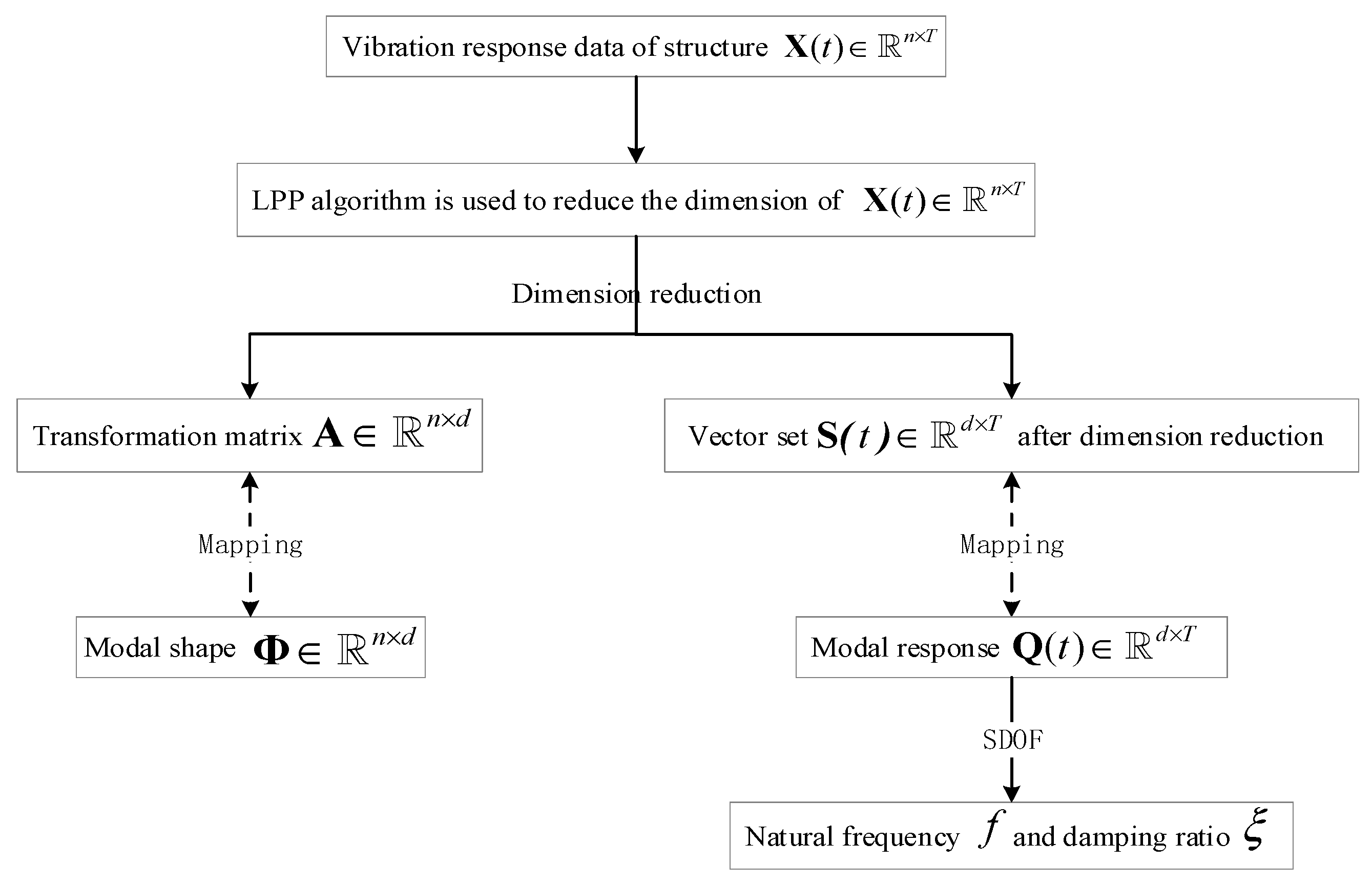
- An operational modal parameter identification method based on LPP is proposed. The main idea is to find out the one-to-one correspondence between the coordinate response matrix and the low-dimensional embedded data, and the one-to-one correspondence between the modal shape matrix and the transformation matrix. The operational modal parameter identification problem can be transformed into the manifold dimension reduction problem of structural vibration response data.
- (2)
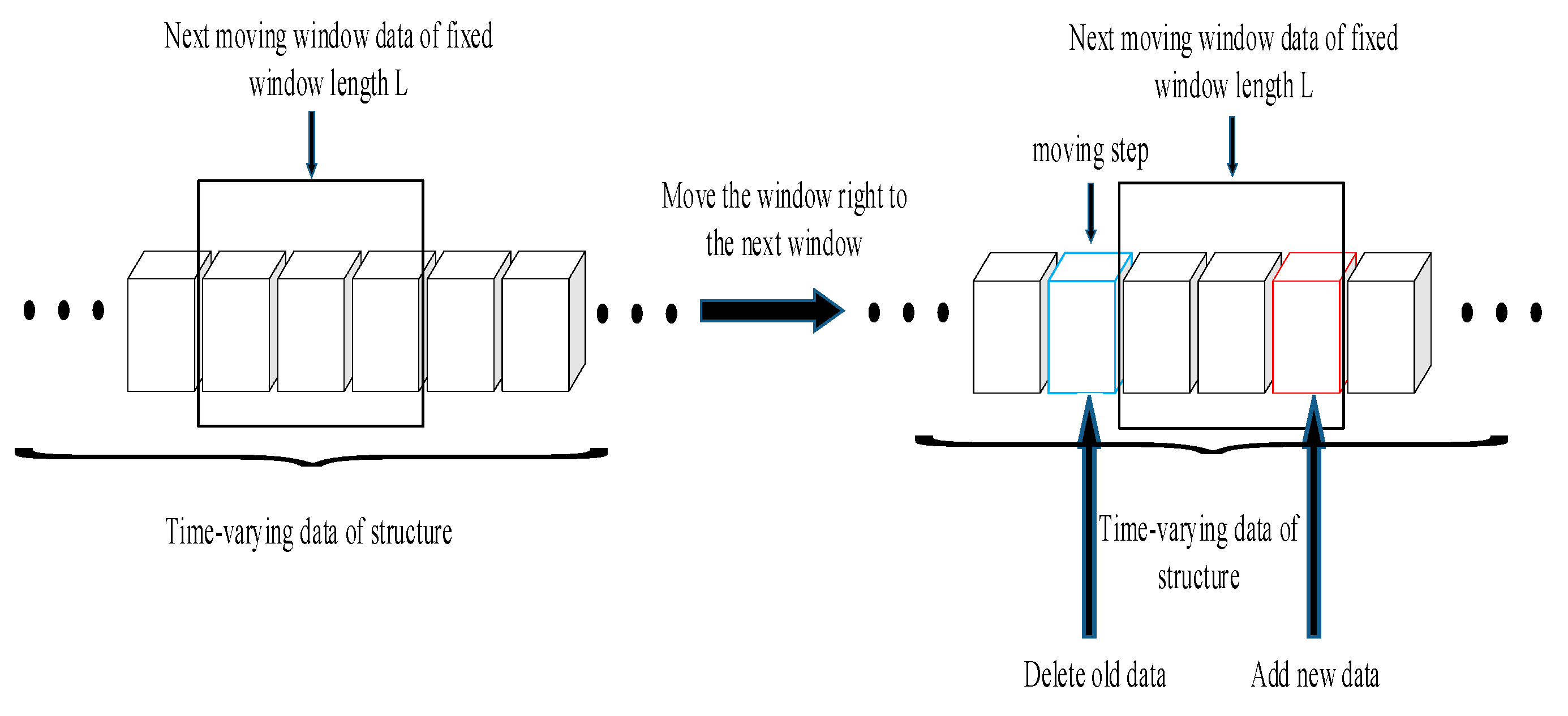
- The LPP algorithm and moving window method are combined to identify the operational modal parameters of linear slow-time-varying structures.
- (3)
- By comparing the operational modal parameter identification method based on moving window principal component analysis method, MWLPP has higher accuracy and effectively reduces the modal missing.
- (4)
- To verify the identification ability of operational modal parameters of linear slow time-varying structures based on MWLPP, a mass slow-time-varying 3-DOF (degree of freedom) structure and a density slow-time-varying cantilever beam structure were designed. The MWPCA method was used to identify the operational modal parameters of non-stationary vibration response simulation data for comparison.
2. OMA of Linear Time-Invariant Structures Based on LPP
2.1. Problem of OMA of Linear Time-Invariant Structures
2.2. OMA of Linear Time-Invariant Structures Based on LPP
- (1)
- Construct an adjacent-graph of T real valued vectors in space: nearest neighbor points of the node are obtained by using the K-neighbor algorithm. If is in the nearest neighbor of , a directed edge (, ) is placed.
- (2)
- Calculate the weight of the edge: let the matrix represents the weight matrix, and is the weight of the edge (, ). The weights of the connected edges are calculated by heat kernel . If the two nodes are not connected, the weight is 0.
- (3)
- Calculate transformation matrix : the eigenvectors and eigenvalues of the generalized eigenvector problem are calculated as follows.where the diagonal matrix is the degree matrix of graph , is the Laplacian matrix.
- (4)
- Let the column vector set correspond to the eigenvector of Equation (5) to be solved, order according to their eigenvalues , The low-dimensional embedded vector of is represented as follows.where Vector satisfies normalized orthogonality.
3. OMA of Linear Time-Varying Structure Based on MWLPP
3.1. Problem of OMA of Linear Time-Varying Structure
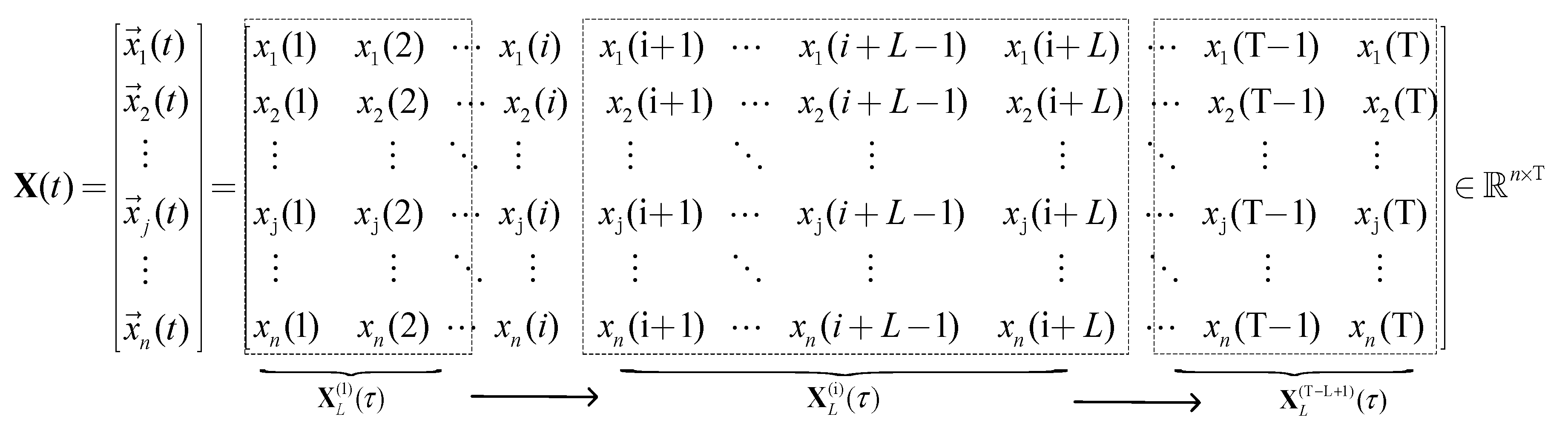
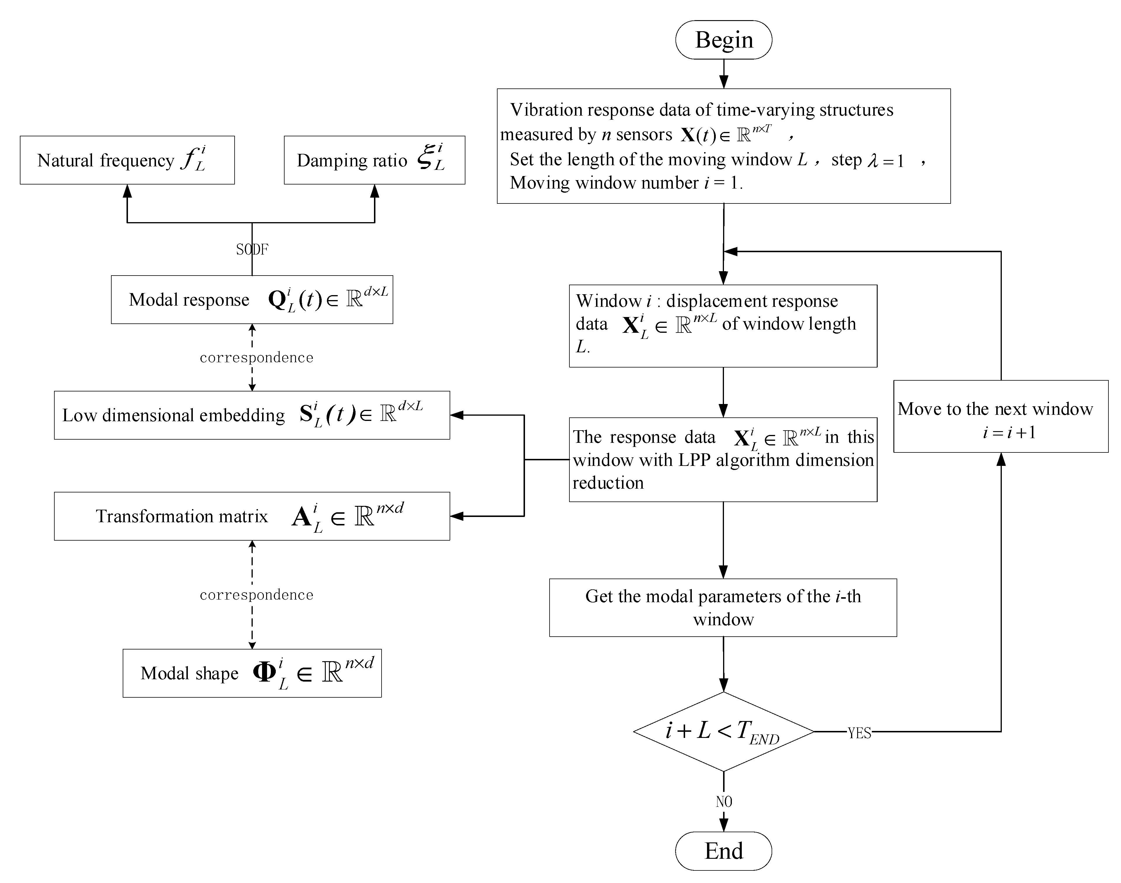
3.2. OMA of Linear Time-Varying Structure Based on MWLPP
3.3. The Applicable Scope of the Method
- (1)
- The method is only suitable for linear slow-time-varying structures with small damping. If the damping is too high, the modals will be complex. Reference [16] show that the damping ratio reaches 10%, and the operational modal parameters can also be identified by manifold learning. However, the lower the damping ratio, the better the identification of modal parameters effect. Only for linear slow-time-varying structures, based on the “time-freezing” theory, Equation (12) can be expressed as Equation (13).
- (2)
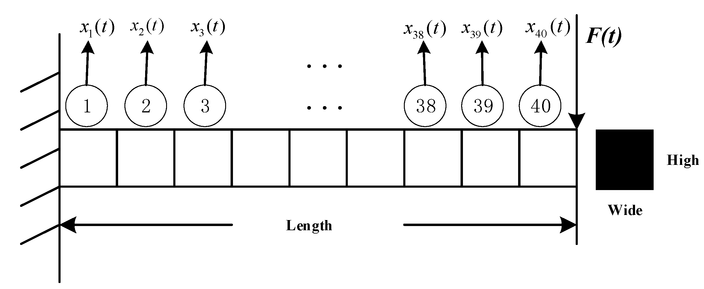
- The number of vibration response sensors n should be greater than or equal to the d-order modal identified by the method. According to Equation (2), the displacement response signal in modal coordinates is approximately represented by d-order modal (). In addition, MWLPP can identify modal natural frequency, modal shape, and damping ratio of one mode with only 1 sensor.
- (3)
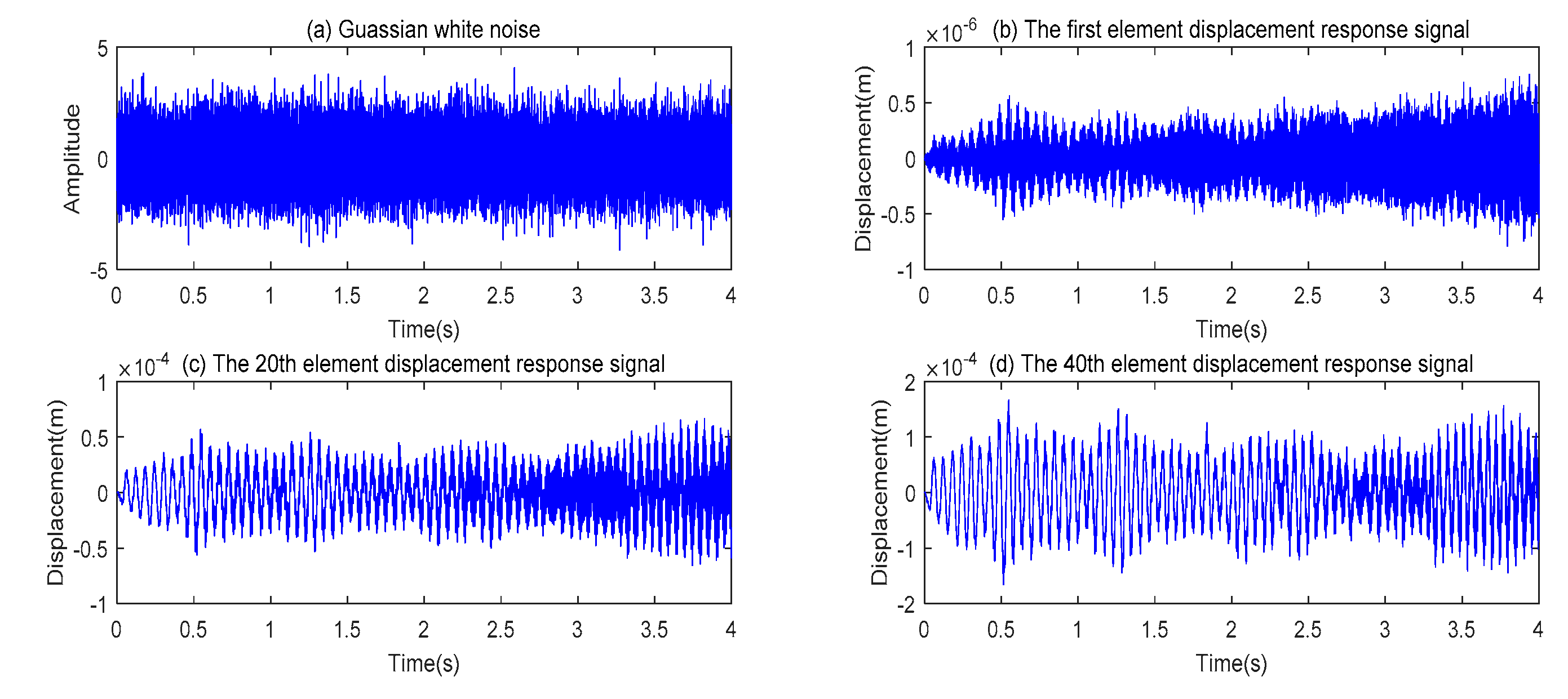
- The excitation vector to the structure should be approximately stationary Gaussian white noise.
- (4)
- The method can identify time-varying transient modal shapes, modal frequencies, and modal damping ratios from non-stationary vibration response signals. However, for linear slow-time-varying structures, mass reduction or motion will generate additional damping [41,42]. Therefore, the damping ratio identified by MWLPP cannot be directly compared with real values.
4. Simulation Verification
4.1. An Introduction to Simulation Systems and Data Sets
4.1.1. A Mass Slow-Time-Varying 3-DOF Structure
4.1.2. A Density Slow-Time-Varying Cantilever Beam Structure
4.2. The Evaluation Indexes
4.3. The Parameter Settings
4.4. Results
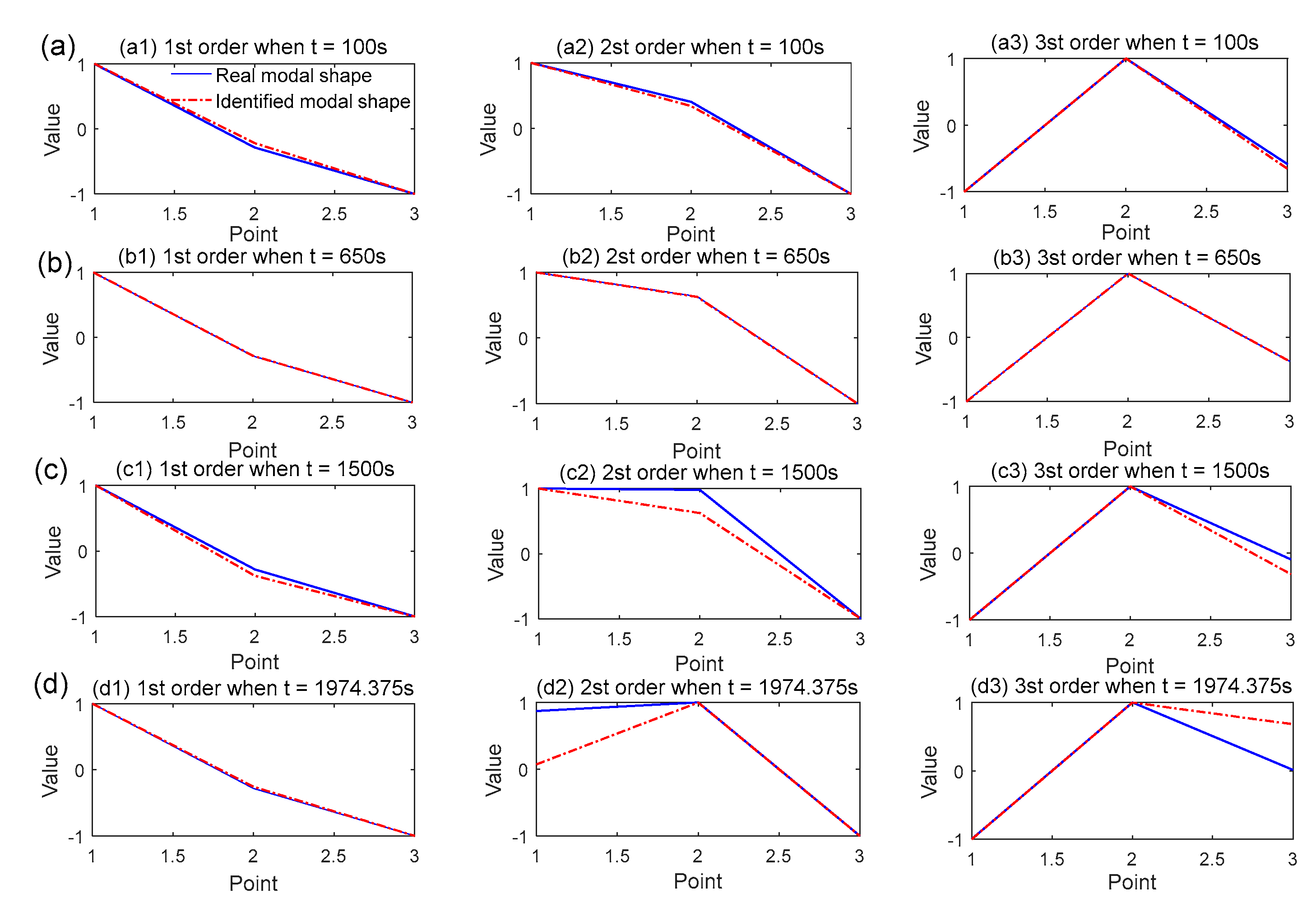
4.4.1. A mass Slow-Time-Varying 3-DOF Structure
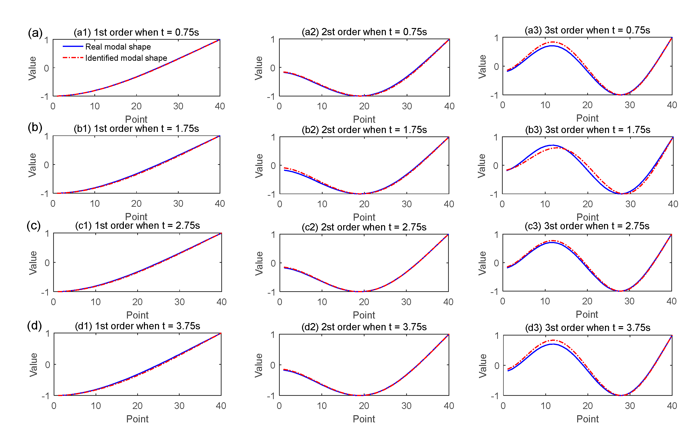
4.4.2. A Density Slow-Time-Varying Cantilever Beam Structure
4.4.3. A Mass Slow-Time-Varying 3-DOF Structure with 10% White Gaussian Noise
4.5. Analysis of Simulation Results
- (1)
- From Figure 12, Figure 13, Figure 14, Figure 15, Figure 16, Figure 17, Figure 18, Figure 19, Figure 20 and Figure 21 and Table 3, Table 4, Table 5, Table 6, Table 7, Table 8, Table 9, Table 10, Table 11, Table 12, Table 13 and Table 14, the MWLPP method can identify the operational modal parameters of the slow time-varying structure well.
- (2)
- (3)
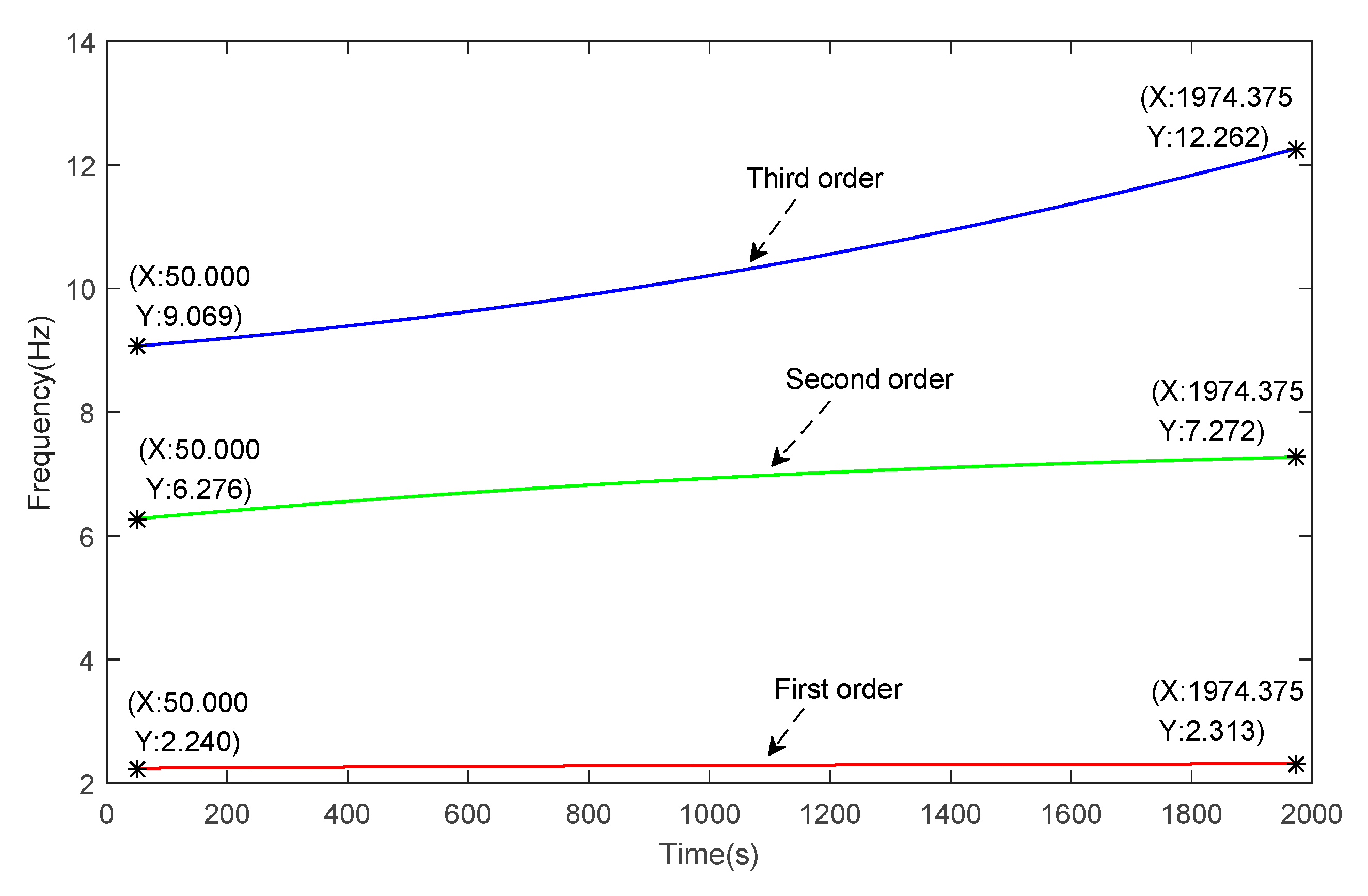
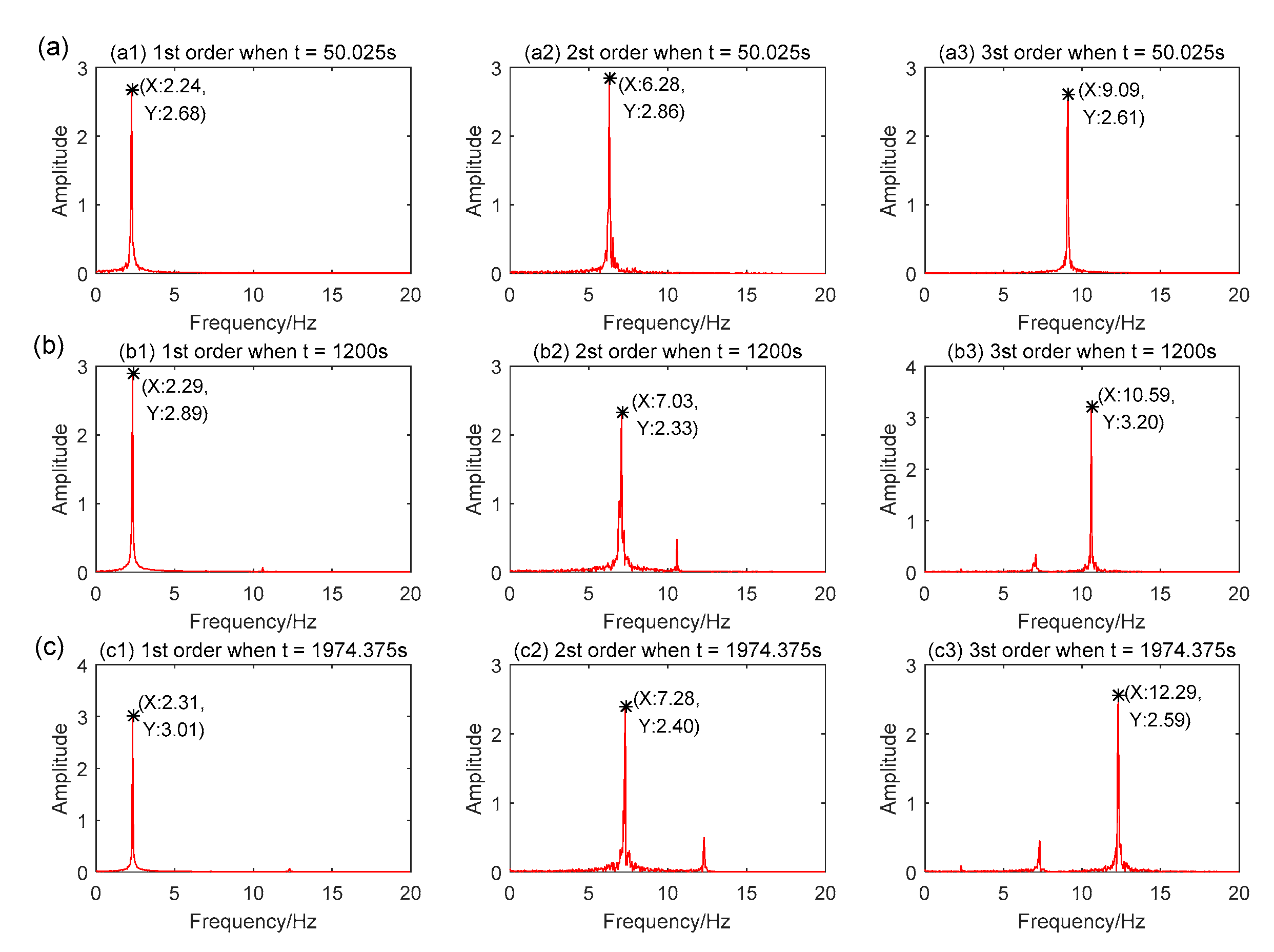
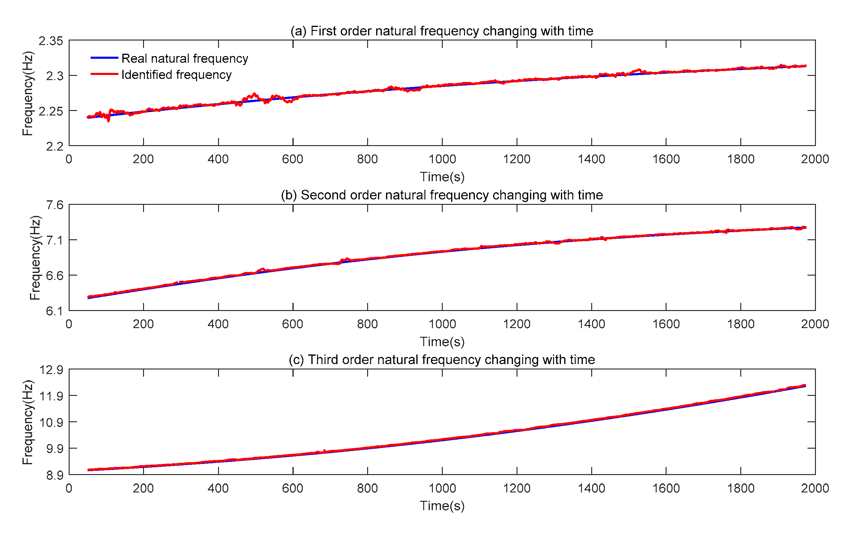
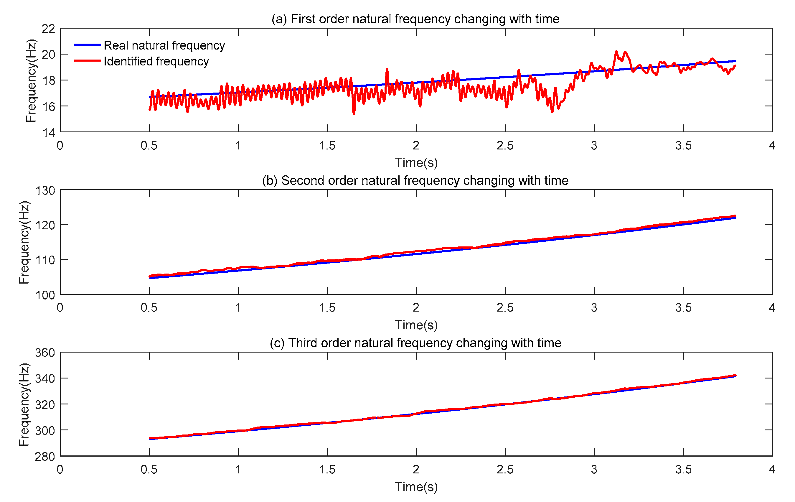
- Comparing Figure 13 and Figure 17, the natural frequency of the linear slow-time-varying structure changing with time, and MWLPP can well track the change of the natural frequency. Combined with Table 4 and Table 8, MWLPP has a high accuracy in identifying the natural frequency of the linear slow-time-varying structure.
- (4)
- Comparing Table 5 and Table 9, the total number of un-identified windows in MWLPP method is lower than that in MWPCA whether the structure is a linear mass slow-time-varying 3-DOF structure or a complex linear density slow-time-varying cantilever beam structure. Comparing Table 6 and Table 10, the MAC value of modal shape identified by MWLPP is higher than that MWPCA. Therefore, the MWLPP method is superior to the MWPCA method in identifying the operational modal parameters of linear slow time-varying structures.
- (5)
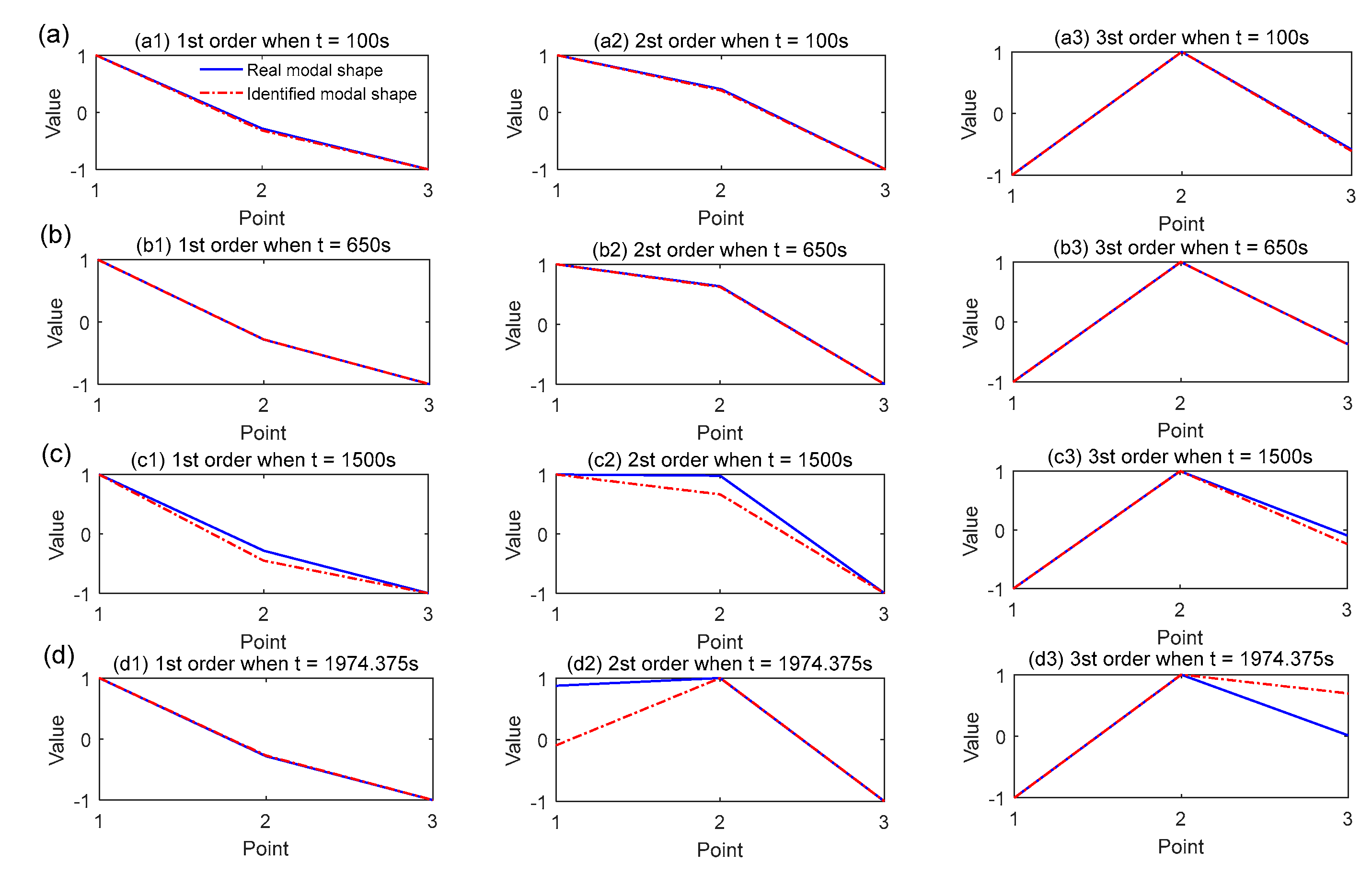
- From Figure 17 and Table 8, the first natural frequency seems contain fluctuations because the ordinate scale of the first mode natural frequency is small. According to Equation (29), in the cantilever beam structure, the first average frequency variation is , the second average frequency variation is , the third average frequency variation is . The smaller the average frequency variation is, the smaller the variation range of the natural frequency value is. Due to the small variation range of the first order natural frequency value, the fluctuation phenomenon of the first order natural frequency is obvious in Figure 15 [28]. In addition, according to Equation (27), the denominator of the first order is much smaller than that of the second and the third order when calculating the average error rate of natural frequency because the natural frequency value of the first order is smaller than that of the second and the third order. Therefore, in Table 8, the average error rate of natural frequency calculated in the first order is greater than that in the second and third order. In fact, the result of modal shape identification shows that the first order identification is indeed the best.
- (6)
- Figure 15 shows that the damping ratio identified by MWLPP algorithm fluctuates greatly because theoretical analysis and numerical simulations indicate that a decreasing or moving mass and density will generate additional damping in the LTV structures [41,42]. In addition, compared with theoretical values, the identification accuracy of damping ratios has a certain error. It is generally predictable because the identification of the damping ratio itself is a difficult problem in the field of structural dynamics, and easily affected by the adopted identification algorithm. Therefore, the time-varying transient mode damping ratio identified by MWLPP is not suitable to compare with the mode damping ratio calculated by finite element methods.
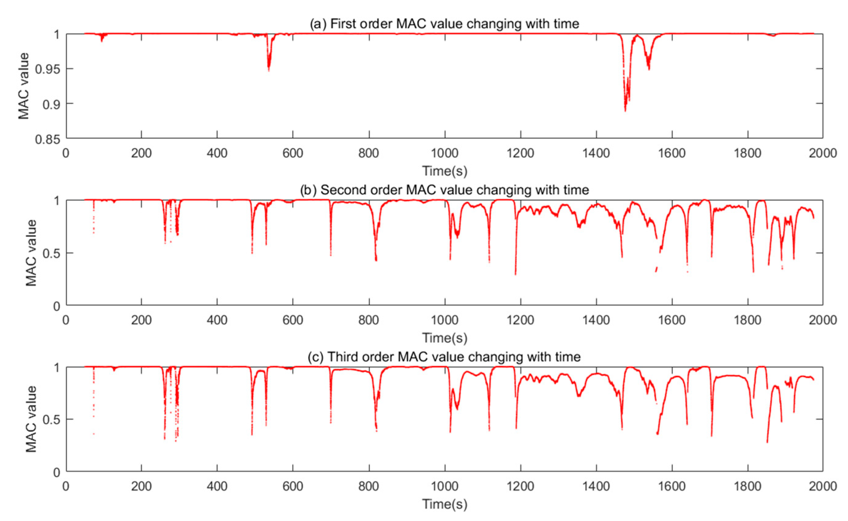
- (7)
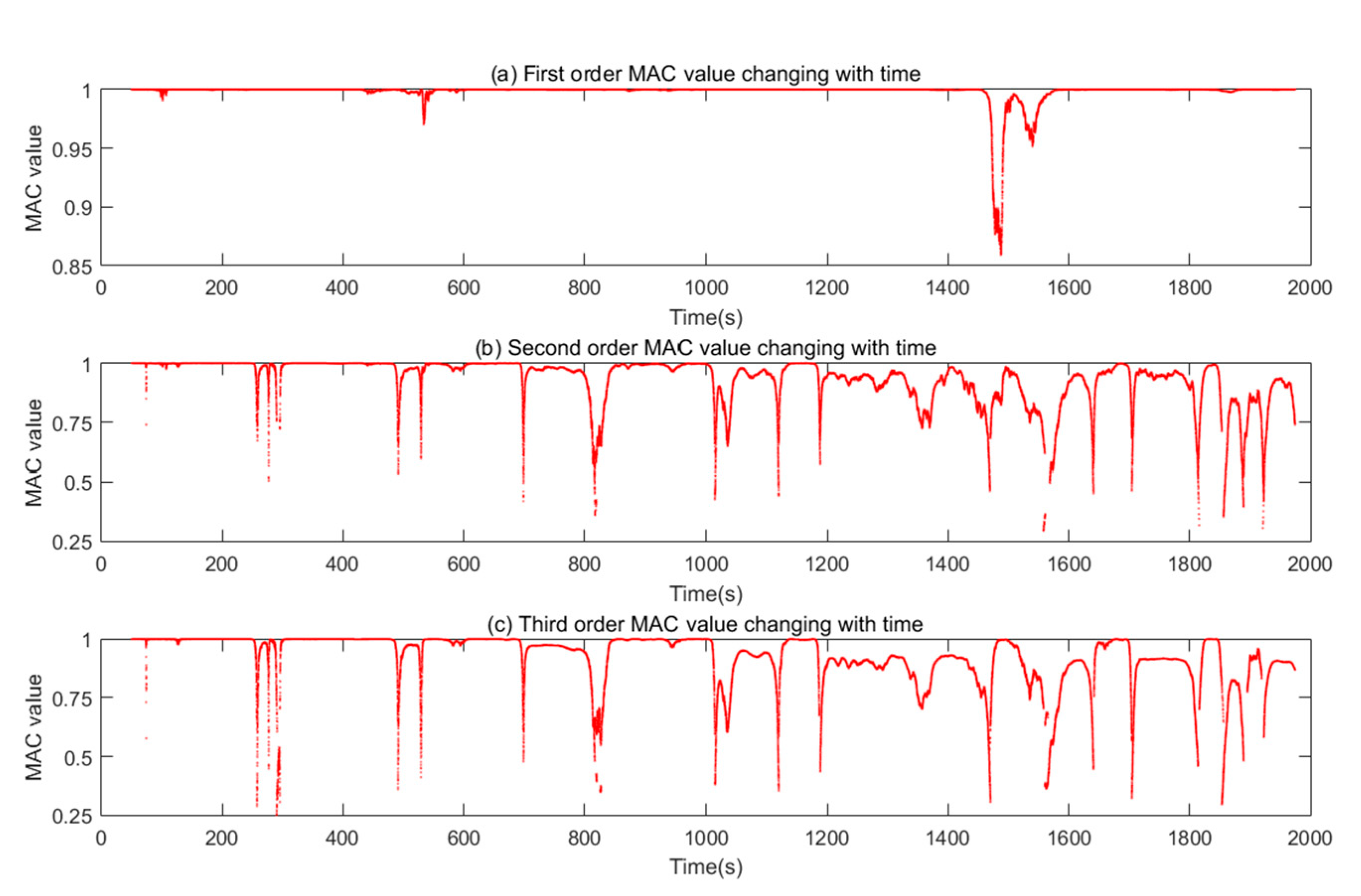
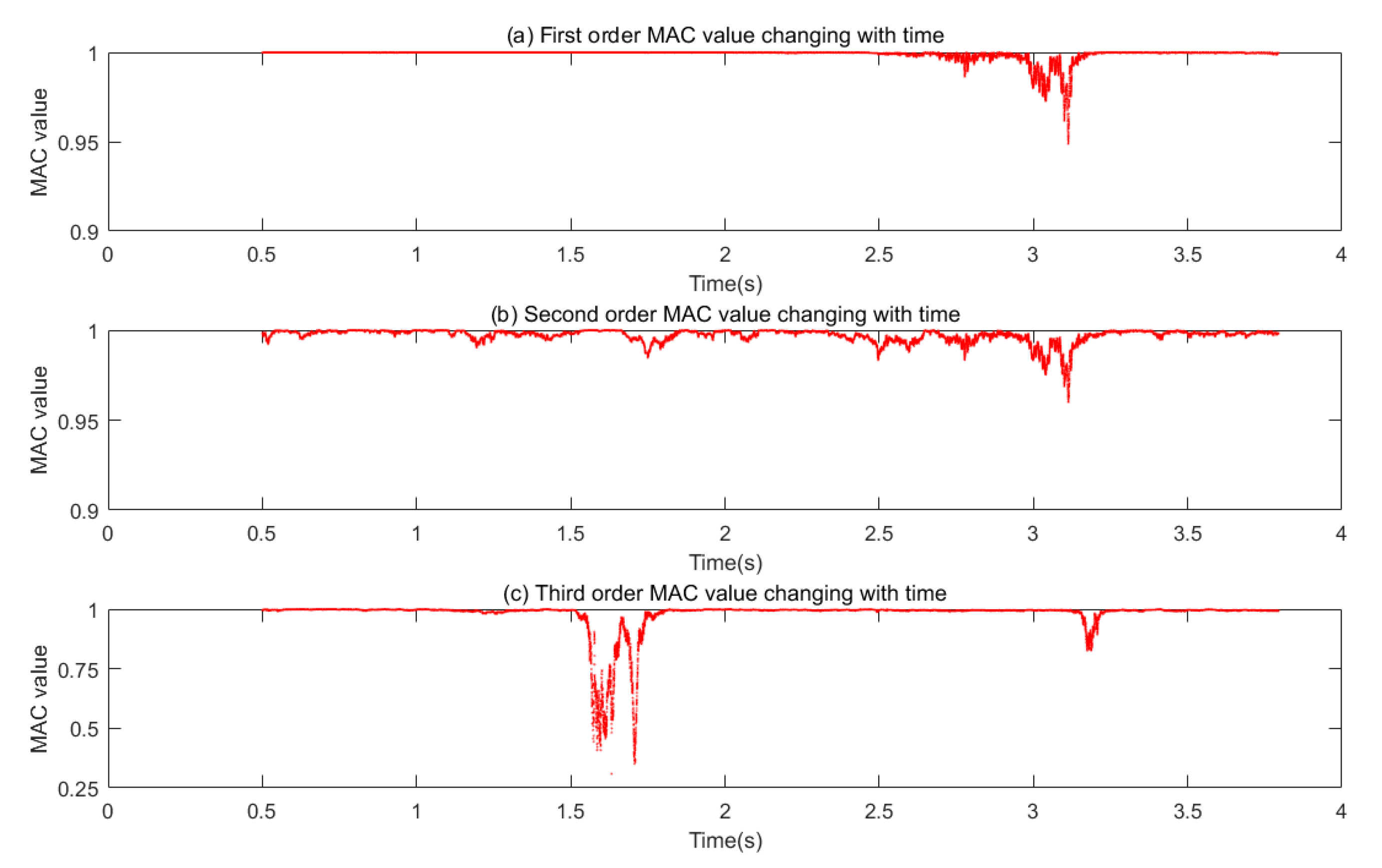
- From Figure 14, Figure 18 and Figure 21, the MAC varies very much and have low values. The time-domain method used in this article cannot use the average technique in the frequency domain to identify the time-domain modes from the non-stationary random vibration response signals. Therefore, the algorithm is unstable, and some moments cannot identify the modal parameters, or the identified modal natural frequency and modal shape are not good. In addition, references [16,43] indicate that the change of damping will affect the performance of the algorithm in identifying modal parameters. From the Figure 15, damping ratio of time-varying structure constantly changing, which leads to low precision of modal parameter identification in some time. In addition, References [28,30] indicate that the window length L will also affect the identification accuracy of modal parameters. From Equation (28), the window length L is proportional to the sample frequency and frequency resolution . Frequency resolution cannot be too small, because it cannot reflect the change of frequency, and cannot be too large, because the average frequency variation cannot be identified. At the same time, cannot be larger too much than , otherwise, time-varying structure cannot be regarded a time-invariant structure in a window.
- (8)
- According to the noise simulation results of 3-DOF structure, the MWLPP algorithm turns out to be robust to noise. This is probably LPP algorithm computes a transformation matrix which maps the data points to a subspace. This linear transformation optimally preserves local neighborhood information in a certain sense [36]. This feature helps retain information about the response signal.
5. Conclusions
Author Contributions
Funding
Institutional Review Board Statement
Informed Consent Statement
Data Availability Statement
Conflicts of Interest
References
- Huang, Z.; Li, Y.; Hua, X.; Chen, Z.; Wen, Q. Automatic Identification of Bridge Vortex-Induced Vibration Using Random Decrement Method. Appl. Sci. 2019, 9, 2049. [Google Scholar] [CrossRef] [Green Version]
- Brandt, A.; Berard, M.; Manzoni, S.; Vanali, M.; Cigada, A. Global scaling of operational modal analysis modes with the OMAH method. Mech. Syst. Signal Process. 2019, 117, 52–64. [Google Scholar] [CrossRef] [Green Version]
- Lee, J. Estimation Modal Parameter Variation with Respect to Internal Energy Variation Based on the Iwan Model. Appl. Sci. 2019, 9, 4290. [Google Scholar] [CrossRef] [Green Version]
- Nagarajaiah, S.; Basu, B. Output only identification and structural damage detection using time frequency and wavelet techniques. Earthq. Eng. Eng. Vib. 2010, 8, 583–605. [Google Scholar] [CrossRef]
- Nabuco, B.; Tarpø, M.; Tygesen, U.; Brincker, R.; Zhao, G. Fatigue Stress Estimation of an Offshore Jacket Structure Based on Operational Modal Analysis. Shock Vib. 2020, 2020, 7890247. [Google Scholar]
- Neu, E.; Janser, F.; Khatibi, A.; Braun, C.; Orifici, A. Operational Modal Analysis of a wing excited by transonic flow. Aerosp. Sci. Technol. 2016, 49, 73–79. [Google Scholar] [CrossRef]
- Aşıkoğlu, A.; Avşar, Ö.; Lourenço, P.B.; Silva, L.C. Effectiveness of seismic retrofitting of a historical masonry structure: Kütahya Kurşunlu Mosque, Turkey. Bull. Earthq. Eng. 2019, 17, 3365–3395. [Google Scholar] [CrossRef]
- Tenenbaum, J.; De-Silva, V.; Langford, J. A global geometric framework for nonlinear dimensionality reduction. Science 2000, 290, 2319–2323. [Google Scholar] [CrossRef]
- Jain, A.; Dubes, R. Algorithms for Clustering Data. Technometrics 1988, 32, 227–229. [Google Scholar]
- Wold, S.; Esbensen, K.; Geladi, P. Principal Component Analysis. Chemometr. Intell. Lab. 1987, 2, 37–52. [Google Scholar] [CrossRef]
- Mukund, B.; Schwartz, E. The Isomap Algorithm and Topological Stability. Science 2002, 295, 7a-7. [Google Scholar]
- Belkin, M.; Niyogi, P. Laplacian Eigenmaps and Spectral Techniques for Embedding and Clustering. Adv. Neural Inf. Process. Syst. 2002, 14, 585–591. [Google Scholar]
- Sam, T.; Lawrence, K. Nonlinear Dimensionality Reduction by Locally Linear Embedding. Science 2000, 290, 2323–2326. [Google Scholar]
- Wang, C.; Gou, J.; Bai, J.; Yan, G. Modal parameter identification with principal component analysis. J. Xi’an Jiaotong Univ. 2013, 47, 97–104. [Google Scholar]
- Bai, J.; Yan, G.; Wang, C. Modal Identification Method Following Locally Linear Embedding. J. Xi’an Jiaotong Univ. 2013, 47, 85–89+100. [Google Scholar]
- Wang, C.; Fu, W.; Huang, H. Isomap-Based Three-Dimensional Operational Modal Analysis. Sci. Program. Neth. 2020, 2020, 1–18. [Google Scholar] [CrossRef]
- Dong, X.; Man, J.; Wang, H.; Yu, S.; Zhao, Y. Structural vibration monitoring and operational modal analysis of offshore wind turbine structure. Ocean Eng. 2018, 150, 280–297. [Google Scholar] [CrossRef]
- Verboven, P.; Cauberghe, B.; Guillaume, P.; Vanlanduit, S.; Parloo, E. Modal parameter estimation and monitoring for on-line flight flutter analysis. Mech. Syst. Signal Process. 2004, 18, 587–610. [Google Scholar] [CrossRef]
- Bart, P.; Herman, V.; Frederik, V.; Patrick, G. Operational modal analysis for estimating the dynamic propertiesof a stadium structure during a football game. Shock Vib. 2007, 14, 283–303. [Google Scholar]
- Poulimenos, A.G.; Fassois, S.D. Parametric time-domain methods for non-stationary random vibration modelling and analysis —A critical survey and comparison. Mech. Syst. Signal Process. 2006, 20, 763–816. [Google Scholar] [CrossRef]
- Zhou, S.; Heylen, W.; Sas, P. Parametric modal identification of time-varying structures and the validation approach of modal parameters. Mech. Syst. Signal Process. 2014, 47, 94–119. [Google Scholar] [CrossRef]
- Zhou, S.; Ma, Y.; Liu, L.; Kang, J.; Ma, Z.; Yu, L. Output-only modal parameter estimator of linear time-varying structural systems based on vector TAR model and least squares support vector machine. Mech. Syst. Signal Process. 2018, 98, 722–755. [Google Scholar] [CrossRef]
- Yang, W. Study on Modal Parameter Estimation and On-Line Identification Technology for Linear Time-Varying Structures in Time-Domain. Ph.D. Thesis, Beijing Institute of Technology, Beijing, China, 2015. [Google Scholar]
- Ramnath, R. Multiple Scales Theory and Aerospace Applications; AIAA: Reston, VA, USA, 2015. [Google Scholar]
- Li, J.; Zhu, X.; Law, S.; Samali, B. Time-varying characteristics of bridges under the passage of vehicles using synchroextracting transform. Mech. Syst. Signal Process. 2020, 140, 106727. [Google Scholar] [CrossRef]
- Kopmaz, O.; Anderson, K. On the Eigenfrequencies of a Flexible Arm Driven by a Flexible Shaft. J. Sound Vib. 2001, 240, 679–704. [Google Scholar] [CrossRef] [Green Version]
- Huang, H.; Wang, C.; Li, H. Moving Window Variable Step-size EASI Based Operational Modal Parameter Identification for Slow Linear Time-varying Structure. Comput. Integr. Manuf. Syst. 2020, 2020, 1–18. [Google Scholar]
- Wang, C.; Wang, J.; Zhang, T. Operational modal analysis for slow linear time-varying structures based on moving window second order blind identification. Signal Process. 2017, 133, 169–186. [Google Scholar] [CrossRef]
- Guan, W.; Wang, C.; Wang, T.; Zhang, H. Operational modal analysis for linear time-varying continuous cantilever beam dynamic structure based on LMPCA. Int. J. Appl. Electrom. 2016, 52, 1–9. [Google Scholar]
- Wang, C.; Guan, W.; Wang, J. Adaptive operational modal identification for slow linear time-varying structures based on frozen-in coefficient method and limited memory recursive principal component analysis. Mech. Syst. Signal Process. 2017, 100, 899–925. [Google Scholar] [CrossRef]
- Wang, C.; Huang, H.; Lai, X.; Chen, J. A New Online Operational Modal Analysis Method for Vibration Control for Linear Time-Varying Structure. Appl. Sci. 2020, 10, 48. [Google Scholar] [CrossRef] [Green Version]
- Du, X.; Wang, F. Modal identification based on Gaussian continuous time autoregressive moving average model. J. Sound Vib. 2010, 329, 4294–4312. [Google Scholar]
- Vu, V.; Thomas, M.; Lakis, A.; Marcouiller, L. Operational modal analysis by updating autoregressive model. Mech. Syst. Signal Process. 2011, 25, 1028–1044. [Google Scholar] [CrossRef]
- Barros, J.; Roux, R.; Lopez, Z.; Martinez, R. Frequency and damping identification in flutter flight testing using singular value decomposition and QR factorization. Proc. Inst. Mech. Eng. Part G J. Aerosp. Eng. 2015, 229, 323–332. [Google Scholar] [CrossRef] [Green Version]
- Chen, Z.; Chan, T.; Nguyen, A.; Yu, L. Identification of vehicle axle loads from bridge responses using preconditioned least square QR-factorization algorithm. Mech. Syst. Signal Process. 2019, 128, 479–796. [Google Scholar] [CrossRef] [Green Version]
- He, X. Locality preserving projections. Adv. Neural Inf. Process. Syst. 2003, 16, 186–197. [Google Scholar]
- Yang, J.; Lei, Y.; Lin, S.; Huang, N. Identification of Natural Frequencies and Dampings of In Situ Tall Buildings Using Ambient Wind Vibration Data. J. Eng. Mech. 2004, 130, 570–577. [Google Scholar] [CrossRef]
- Kerschen, G.; Poncelet, F.; Golinval, J. Physical interpretation of independent component analysis in structural dynamics. Mech. Syst. Signal Process. 2007, 21, 1561–1575. [Google Scholar] [CrossRef]
- Poncelet, F.; Kerschen, G.; Golinval, J.; Verhelstet, D. Output-only modal analysis using blind source separation techniques. Mech. Syst. Signal Process. 2007, 21, 2335–2358. [Google Scholar] [CrossRef]
- Klepka, A.; Uhl, T. Identification of modal parameters of non-stationary systems with the use of wavelet based adaptive filtering. Mech. Syst. Signal Process. 2014, 47, 21–34. [Google Scholar] [CrossRef]
- Ma, C.; Zhang, X.; Luo, Y. Dynamic analysis on a fluid-structure coupling system with variable mass in a rectangular tank. J. Xi’an Jiaotong Univ. 2014, 48, 109–116. [Google Scholar]
- Ma, C.; Zhang, X.; Luo, Y.; Zhang, S. Dynamic responses for a fluid-structure coupling system with variable mass in a tank of spacecraft. J. Aerosp. Power 2015, 330, 736–745. [Google Scholar]
- Zhou, W.; Chelidze, D. Blind source separation based vibration mode identification. Mech. Syst. Signal Process. 2007, 21, 3072–3087. [Google Scholar] [CrossRef]


| Real Natural Frequency (Hz) | |||
|---|---|---|---|
| Order | t = 50.025 s | t = 1200 s | t = 1974.375 s |
| 1 | 2.24 | 2.29 | 2.31 |
| 2 | 6.28 | 7.02 | 7.27 |
| 3 | 9.07 | 10.56 | 12.26 |
| Real Natural Frequency (Hz) | |||
|---|---|---|---|
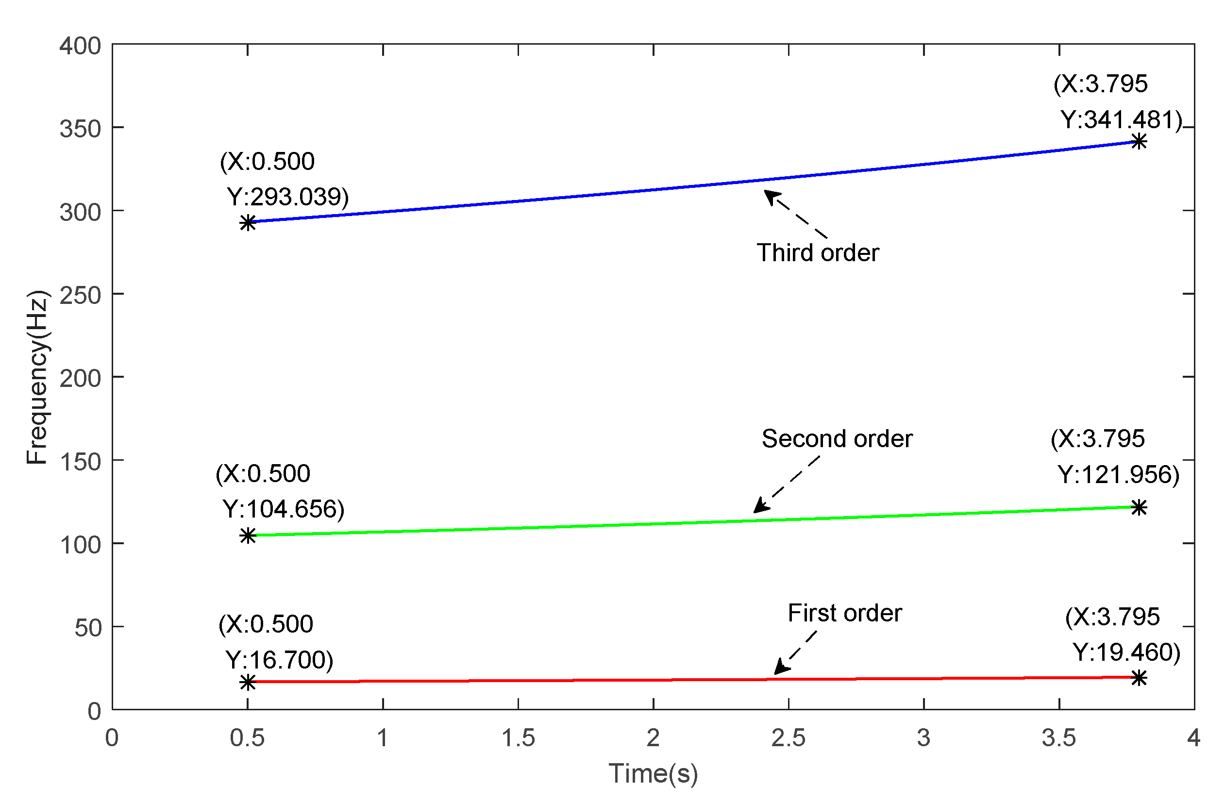
| Order | t = 0.5 s | t = 2 s | t = 3.795 s |
| 1 | 16.70 | 17.80 | 19.46 |
| 2 | 104.66 | 111.56 | 121.96 |
| 3 | 293.03 | 312.38 | 341.48 |
| Order | t = 100 s | t = 650 s | t = 1500 s | t = 1974.375 s |
|---|---|---|---|---|
| 1 | 1 | 1 | 0.9908 | 1 |
| 2 | 0.9999 | 0.9988 | 0.9746 | 0.7391 |
| 3 | 0.9998 | 1 | 0.9908 | 0.8691 |
| Method | |||
|---|---|---|---|
| MWLPP | 0.059% | 0.128% | 0.244% |
| MWPCA | 0.059% | 0.129% | 2.45% |
| Method | First Order Un-Identified Number | Rate | Second Order Un-Identified Number | Rate | Third Order Un-Identified Number | Rate |
|---|---|---|---|---|---|---|
| MWLPP | 0 | 0 | 808 | 1.049% | 747 | 0.970% |
| MWPCA | 0 | 0 | 746 | 0.969% | 1827 | 2.373% |
| Method | |||
|---|---|---|---|
| MWLPP | 0.9979 | 0.9344 | 0.9254 |
| MWPCA | 0.9982 | 0.9009 | 0.9052 |
| Order | t = 0.75 s | t = 1.75 s | t = 2.75 s | t = 3.75 s |
|---|---|---|---|---|
| 1 | 1 | 0.9998 | 0.9999 | 0.9997 |
| 2 | 0.9981 | 0.9858 | 0.9990 | 0.9988 |
| 3 | 0.9951 | 0.9742 | 0.9975 | 0.9947 |
| Method | |||
|---|---|---|---|
| MWLPP | 3.234% | 0.469% | 0.159% |
| MWPCA | 3.07% | 0.470% | 0.161% |
| Method | First Order Un-Identified Number | Rate | Second Order Un-Identified Number | Rate | Third Order Un-Identified Number | Rate |
|---|---|---|---|---|---|---|
| MWLPP | 0 | 0 | 6 | 0.018% | 124 | 0.376% |
| MWPCA | 213 | 0.64% | 1 | 0.003% | 66 | 0.2% |
| Method | |||
|---|---|---|---|
| MWLPP | 0.9990 | 0.9971 | 0.9789 |
| MWPCA | 0.9834 | 0.9773 | 0.8996 |
| Order | t = 100 s | t = 650 s | t = 1500 s | t = 1974.375 s |
|---|---|---|---|---|
| 1 | 0.9995 | 1 | 0.9938 | 1 |
| 2 | 0.9988 | 0.9997 | 0.9707 | 0.8243 |
| 3 | 0.9970 | 1 | 0.9818 | 0.8731 |
| Method | |||
|---|---|---|---|
| MWLPP (with 10% white Gaussian noise) | 0.059% | 0.127% | 0.245% |
| MWLPP(without white Gaussian noise) | 0.059% | 0.129% | 2.45% |
| Method | First Order Un-Identified Number | Rate | Second Order Un-Identified Number | Rate | Third Order Un-Identified Number | Rate |
|---|---|---|---|---|---|---|
| MWLPP (with 10% white Gaussian noise) | 0 | 0 | 674 | 0.876% | 1062 | 1.380% |
| MWLPP (without white Gaussian noise) | 0 | 0 | 808 | 1.049% | 747 | 0.970% |
| Method | |||
|---|---|---|---|
| MWLPP (with 10% white Gaussian noise) | 0.9981 | 0.9260 | 0.9219 |
| MWLPP (without white Gaussian noise) | 0.9979 | 0.9344 | 0.9254 |
Publisher’s Note: MDPI stays neutral with regard to jurisdictional claims in published maps and institutional affiliations. |
© 2021 by the authors. Licensee MDPI, Basel, Switzerland. This article is an open access article distributed under the terms and conditions of the Creative Commons Attribution (CC BY) license (http://creativecommons.org/licenses/by/4.0/).
Share and Cite
Fu, W.; Wang, C.; Chen, J. Operational Modal Analysis for Vibration Control Following Moving Window Locality Preserving Projections for Linear Slow-Time-Varying Structures. Appl. Sci. 2021, 11, 791. https://doi.org/10.3390/app11020791
Fu W, Wang C, Chen J. Operational Modal Analysis for Vibration Control Following Moving Window Locality Preserving Projections for Linear Slow-Time-Varying Structures. Applied Sciences. 2021; 11(2):791. https://doi.org/10.3390/app11020791
Chicago/Turabian StyleFu, Weihua, Cheng Wang, and Jianwei Chen. 2021. "Operational Modal Analysis for Vibration Control Following Moving Window Locality Preserving Projections for Linear Slow-Time-Varying Structures" Applied Sciences 11, no. 2: 791. https://doi.org/10.3390/app11020791
APA StyleFu, W., Wang, C., & Chen, J. (2021). Operational Modal Analysis for Vibration Control Following Moving Window Locality Preserving Projections for Linear Slow-Time-Varying Structures. Applied Sciences, 11(2), 791. https://doi.org/10.3390/app11020791