Assuming a perpendicular imaging angle, the mm length of an object can be measured accurately. Accurate estimation of the mm length of an object from the pixel length of the object’s image is the primary goal of calibrated horizontal measurement. Assuming an optical system that is symmetrical around its optical axis, the relationship between an object and its image can be determined. Let
denote the mm length of an object and
denote the pixel length of the object’s image. Also, let O be the intersection point between a ray of light from the object and the lens of the camera (
Figure 1) expressed in the polar coordinates (
, φ). We would have [
29],
where A
j and B
j are constants, and HOT represents the higher-order terms. Readers interested in more detailed analysis of image formation may refer to [
29] and its references.
Equation (1) shows a non-linear and complex relationship between pixel and mm lengths. Using the thin-lens assumption and small-angle approximation [
29] Equation (1) can be approximated with a much simpler model known as the Gaussian optics [
29]. In this model, the ratio of pixel length to mm length is a constant number, which is called the magnification factor of the system (m). Equation (2) shows the following:
Flexible fiberoptic endoscopes employ wide-angle lenses to maximize their FOV sizes. However, wide-angle lenses violate the small-angle approximation of the Gaussian optics. This leads to a more complex relationship between pixel and mm lengths. Specifically, this deviation introduces significant non-linear distortion into recorded images. Recently, Ghasemzadeh et al. [
14] studied the distortion of a flexible laryngoscope and showed that when the imaging axis is perpendicular to the target surface, the distortion is symmetrical around the optical axis, and points with similar distances from the FOV center experience similar distortions. Considering this symmetry, Equation (1) may govern the image formation in flexible endoscopy. Additionally, that study showed the pixel length of an object significantly depends on its spatial location within the FOV [
14]. Therefore, the spatial location of the target object is another confounding factor for horizontal measurements. Circular grids can exploit this symmetry efficiently; thus, the proposed method uses circular grids to account for the effect of working distance and the spatial location of the target object.
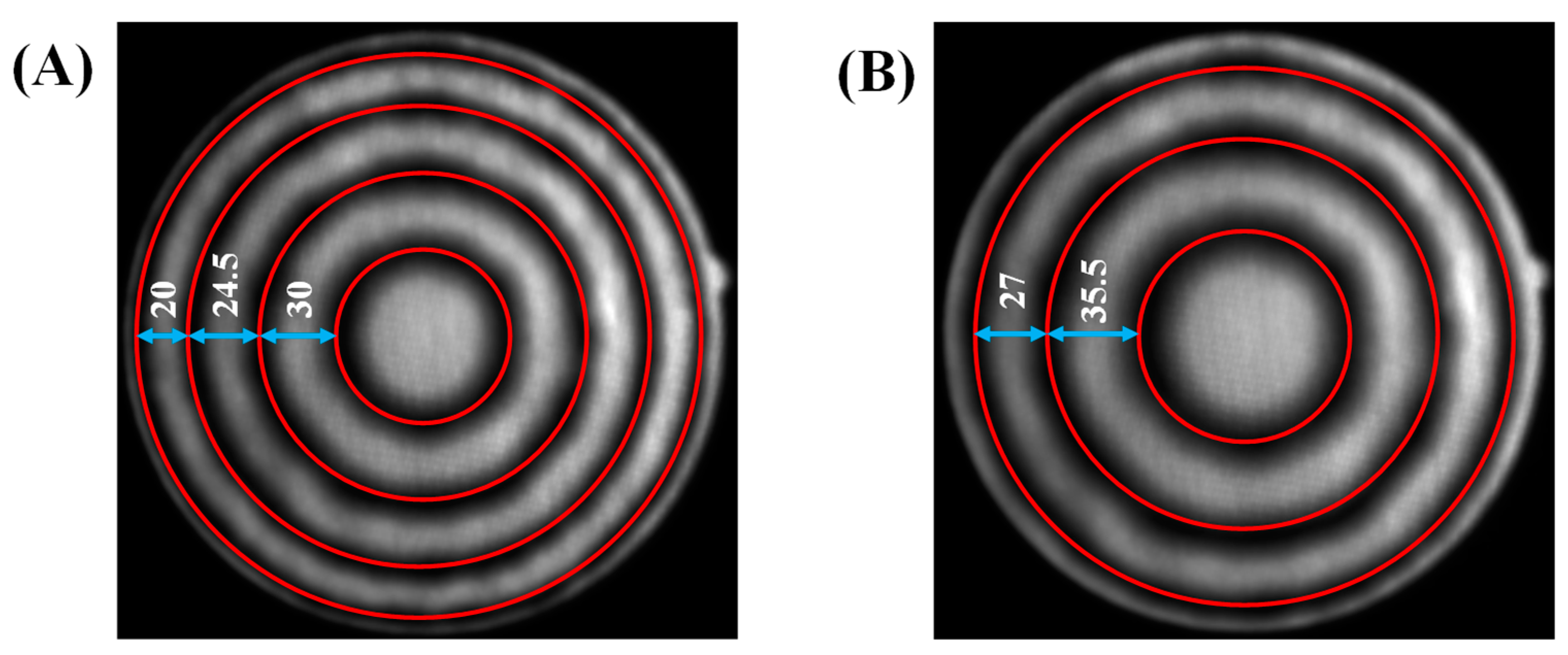
To demonstrate this, a circular grid with the spacing of 0.5 mm was recorded at working distances of 2.87 mm and 2.24 mm.
Figure 2 shows the recorded images. The circles had a constant distance of 0.5 mm from each other. However, in
Figure 2A we see as we go from the center toward the periphery the distance between consecutive circles decreases from 30 pixels to 20 pixels. This clearly demonstrates the dependence of horizontal measurements on the spatial location. Comparing
Figure 2A,B we see the effect of working distance, where the distance between the two smallest circles increases from 30 pixels to 35.5 pixels when the working distance decreases from 2.87 mm (
Figure 2A) to 2.24 mm (
Figure 2B).
2.1. Recording Instrumentation and Setup
The data acquisition system consisted of a custom-built laser-projection flexible endoscopy system [
20] attached to a high-speed monochrome Phantom v7.1 camera (Vision Research Inc., Wayne, NJ, USA). The laser-projection endoscope was based on the surgical fiberoptic endoscope, Fiber Naso Pharyngo Laryngoscope Model FNL-15RP3 (PENTAX Medical, Montvale, NJ, USA). The surgical channel of the endoscope was used for housing of the optical components of the laser projection system and delivering the laser pattern on the FOV. A diffraction-based design was used to create a 7 × 7 grid pattern from a 520 nm green-laser beam [
20].
The proposed calibration and subsequent horizontal measurement methods were developed and then evaluated based on different sets of benchtop recordings. The employed setup consisted of an adjustable arm for precise tuning of the distance between the distal tip of the endoscope and the target surface (i.e., working distance) [
14,
24]. A digital height gauge with an accuracy of 0.001 inch (0.025 mm) was used for measurement of the working distance. All recordings were carried out at a spatial resolution of 288 × 280 pixels and speed of 100 frames per second. Considering that images were taken from static surfaces, this frame rate was irrelevant, where 100 fps was an adequate rate for our purpose [
14].
2.2. Datasets
This study used four different sets of recordings. Set 1 contained 65 recordings from circular grids (
Figure 2) at different working distances. This set was used for training and testing of the model converting a pixel length to its mm length. The working distance was gradually increased from 2 to 32 mm. This range covers the working distances applicable to laryngeal flexible endoscopy. At each working distance, a recording was done. This process was repeated three times to reduce measurement error. For each recording, the grid was adjusted subjectively inside the FOV such that the largest visible circle had a uniform distance from the border of the FOV. Considering the limited spatial resolution, grids became significantly blurry after a certain working distance. Hence, three different circular grids with the spacing of 0.5, 1, and 2 mm were used for working distances in the range of [2,10], [10,20], and [20,32] mm. The presence of the laser points was saturating some of the black pixels belonging to the grids. This could affect accurate detection of the grid. Also, the laser points were not necessary for the purpose of this set; therefore, the laser source was turned off during these recordings.
The proposed method requires an accurate estimation of the distance between the tip of the endoscope and the target surface (i.e., the working distance). Previously, it was shown that a statistical model can be trained to decode the working distance from locations of the laser points [
24]. Set 2 had 72 recordings and was used for the training of the model that estimates the working distance. For this set, the laser source was turned on, and the light source was turned off and recordings were done from a white paper. The working distance was gradually increased from 2 to 35 mm and at each working distance, a recording was done. The recording process was repeated four times to reduce measurement error.
The proposed method relies on an accurate estimation of a central angle (i.e., an angle that has its apex on the center of a circle). However, flexible endoscopy images exhibit significant nonlinear distortions [
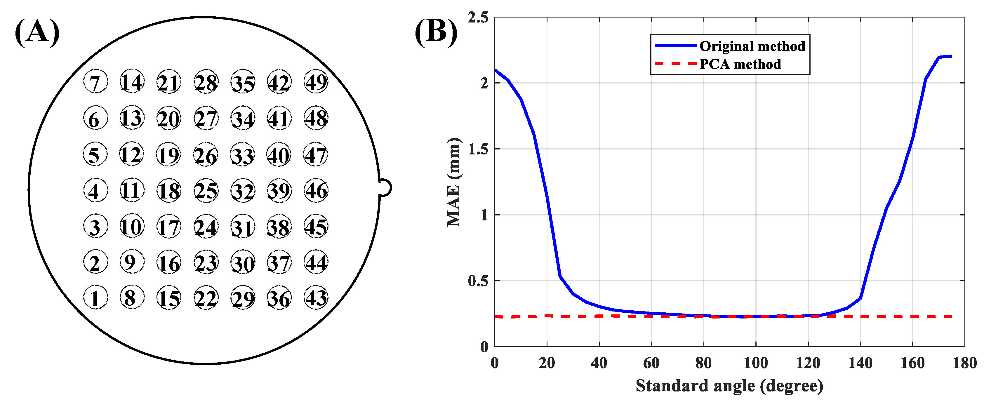
14]. Set 3 was recorded to investigate possible effects of the introduced nonlinear distortion on central angle measurements. This set was based on a custom-designed grid. A circular grid was divided into 24 equal sectors, which created 24 central angles in 15° increments (
Figure 3A). The grid was recorded at four working distances of 6.16, 13.20, 19.54, and 26.44 mm. At each recording distance, the grid was adjusted subjectively inside the FOV such that the largest visible circle had a uniform distance from the border of the FOV. This process insured that the center of the grid was at the center of the FOV. This characteristic governs that estimated angles from the image are central angles. The laser source was turned off during these recordings.
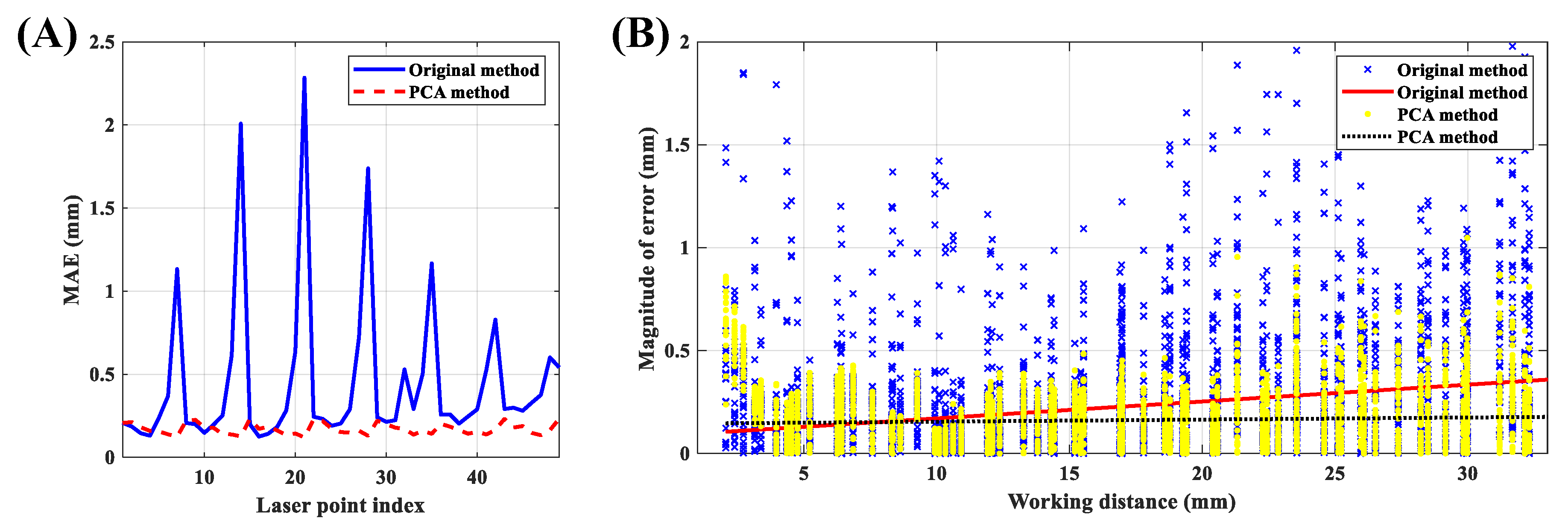
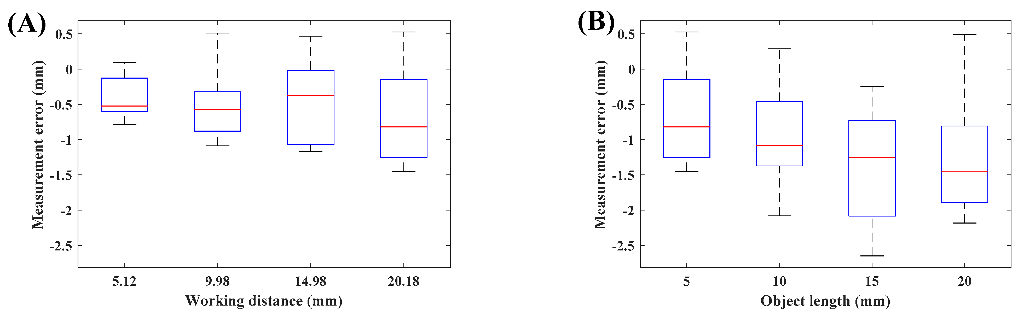
Set 4 was recorded for evaluating the accuracy of the proposed method. Line segments with known mm lengths were recorded at fifteen arbitrary locations in the FOV with arbitrary rotations. To provide a comprehensive evaluation, a wide range of lengths and working distances were used. Specifically, 5, 10, 15, and 20 mm line segments were recorded at a working distance of 20.18 mm. These recordings were used to investigate the possible effect of object length on the accuracy of the method. Additionally, a 5 mm line segment was recorded at working distances of 5.12, 9.98, 14.98, and 20.18 mm, which covers the common range of administration of fiberoptic laryngeal endoscopy. These recordings were used to investigate the possible effect of working distance on the accuracy of the method. The laser source was turned on during these recordings.
Figure 3C presents an example from Set 4.
Table 1 presents a summary of each data set.
2.3. Segmentation and Preprocessing
Accurate detection of circular grids is a prerequisite of the proposed calibration method. An automatic two-stage method was developed for the segmentation of the circles from Set 1. To take advantage of the full 72 dB dynamic range of the camera, recordings were imported into MATLAB (MathWorks, Natick, MA, USA) directly in the native 12-bit format from the proprietary Vision-Research .cine (Vision Research Inc., Wayne, NJ, USA) files without any conversion or compression. To reduce the noise of images, frames of the recordings were averaged over time and then a Gaussian filter with a size of 2 pixels was applied. The Center and radius of the FOV were estimated using the method described in [
24]. A strip parallel to the x-axis centered at the center of the FOV with a width of nine pixels was selected. The strip was averaged over the rows, and then locations of its local minima were detected. Detected locations were paired based on their distances from the center of the FOV. The average of each pair was used as the coarse estimation of the x-coordinate of centers of circles. Half of the difference between each pair was used as the row-wise estimation of radii of circles. This process was repeated for a strip parallel to the y-axis averaged over the columns. The average of each pair was used as the coarse estimation of the y-coordinate of centers of circles. Half of the difference between each pair was used as the column-wise estimation of radii of circles. The final coarse estimation of the radius of each circle was computed as the average of its row- and column-wise radii. A grid search over all combinations of the three estimated parameters ±1 pixel with the resolution of 0.25 pixels was used for fine-tuning of the estimated parameters. Specifically, for each case, the target parameters were used to create a ring mask with a width of 1 pixel. The mask was then applied to the gradient of the image, and the summation of the results was used as the cost function. The set of parameters that minimized the cost function was selected as the final estimation of the center and radius of each circle.
Figure 4 shows the process, with the results on an example image.
The segmentation of the laser points for Set 2 was based on the method described in [
24]. Target objects in Set 3 were 24 radial lines, which were detected using the Hough transform [
30].
Figure 3B shows the grid after segmentation. The actual horizontal measurements on laryngeal images will rely on the manual segmentation of the target object. To better reflect this, a graphical user interface was developed for manual segmentation of line segments from Set 4.
2.4. Horizontal Calibration Method
Working distance and spatial location of the target object are the main confounding factors of horizontal measurements. Circular grids provide an effective way for the spatial sampling of the location inside the FOV. This information can be utilized for determining the dependence of horizontal measurements on the spatial location. Additionally, the grids can be recorded at multiple working distances. This information may be utilized for determining the dependence of horizontal measurements on the working distance. To that end, all circles from Set 1 were segmented. Obviously, depending on the working distance different numbers of circles will fall inside the FOV, and hence will be recorded. The segmentation process of all 65 recordings resulted in 612 different data points. Let
,
, and
denote the working distance, pixel radius, and mm radius of a circle, respectively, recorded at
mm. Then, a statistical model can be trained using
and
as the predictor variables and
as the outcome variable. Let
denote a polynomial model in two variables,
and
, with maximum degrees of M and N, respectively. Equations (3) and (4) show the model, where
are some constants determined during the training process:
To select the best model, polynomial models with different degrees were evaluated using 10-fold cross-validation. The cost function was defined as the mean absolute error (MAE) over all testing samples from all 10 folds. The
resulted in the MAE of 0.025 mm, which was the lowest value. This model will be referred to as the non-uniform model in the rest of this paper.
Figure 5A presents the trained non-uniform model.
To highlight the effect of spatial location on horizontal measurements, a second model was trained where all pixels in the FOV had similar pixel sizes. This scenario mimics horizontal measurement from a parallel-laser projection system. Let,
and
denote the pixel radius and mm radius of the largest circle visible in the FOV recorded at the working distance of
mm. The uniform pixel size
is defined as
The uniform pixel size was computed for all recordings in Set 1. Then, a statistical model was trained using the working distance as the predictor variable and
as the outcome variable. Investigating the relationship between working distance and
revealed a linear model. This model is shown in
Figure 5B and it will be referred to as the uniform model in the rest of this paper.
2.5. Horizontal Measurement Method
The application of the uniform model is simple and quite similar to the estimation of a distance on a printed map. The pixel size (
) allows the conversion from pixel length into mm length. Considering the dependence of
on the working distance, the following steps were followed for horizontal measurements using the uniform model. The working distance was estimated from the positions of the laser points [
24]; then the appropriate value of the pixel size was computed from the uniform model. The pixel length of the target object was measured on the image; then the pixel length was multiplied with the multiplicative factor of pixel size to estimate its mm length.
The application of the non-uniform model is more involved, and it is described under two categories of radial and general measurements. A radial measurement is defined as the length of an object that has one of its ends on the FOV center. The non-uniform model was trained using circles centered at the FOV center. Therefore, the model can estimate the mm radius of a circle centered at the FOV center, which would be equivalent to a radial measurement. Thus, the following steps were followed for horizontal radial measurements using the non-uniform model. The working distance was estimated from the positions of the laser points [
24]. Then, the pixel length of the target radial object was measured on the image. The values of working distance and pixel length were fed into the trained non-uniform model (Equation (3)), and the mm length of the object was estimated.
A general measurement needs to be expressed in terms of radial measurements before the application of the non-uniform model.
Figure 6 shows this process. The main goal is to determine the length of the line segment AB in mm. We can construct the triangle AOB on the image, where O is the FOV center. Referring to
Figure 6, OA and OB each has one of their ends at the FOV center, and hence they constitute radial measurements, and their mm lengths can be computed using the non-uniform model. At the same time, we can measure the angle α from the image. Let
and
on the image, then, we can determine the angle between OA and the positive x-axis (
) as follows,
where
denotes the four-quadrant inverse tangent function. The angle between OB and the positive x-axis (
) can also be measured, similarly. Finally, the angle α can be computed as,
Now, we can apply the law of cosines for determining the mm length of the line segment AB:
2.6. Estimation of the Working Distance
Referring to Equations (3) and (5), we see that accurate estimation of the working distance is a prerequisite of both uniform and non-uniform methods. The method for estimating the working distance has been presented in [
24]. The method is described very shortly here, followed by an improvement over the previous approach. The position of a laser point is a function of the working distance, once the effect of magnification and rotation and displacement of the FOV are compensated for [
24]. Therefore, we may train a statistical model that could decode the working distance from the position of a laser point. In [
24], this was achieved by converting the position of the laser point from the Cartesian coordinate system into the polar coordinate system. Then, the radius component (r) of the position of the laser point was used for the training of the model. Equations (9) and (10) show the model (
), where
is the radius computed from the laser point i at the working distance
, and
are some constants determined during the training process:
The original model also assumed that the data were mapped into a standard template by applying a chain of rotation, translation, and scaling operations on the recorded images. Flexible endoscopes have a fiducial marker (see, e.g., protrusion on right side of circle in
Figure 4 and
Figure 6) that helps with the orientation of the recorded images. The rotation operation was parametrized in terms of the angle between the positive x-axis and the line connecting the fiducial marker to the FOV center. The rotation operation brings this angle to a fixed and standard value across all recordings [
24]. This value will be further termed standard angle. In essence, the standard angle it is the angle between the fiducial marker and the x-axis of the image after undergoing the rotation operation. For example, the standard angle of
Figure 6 is zero degrees. First, we show that the performance of the original method depends on the value of this angle; then we propose an improved version to alleviate this problem.
Ten-fold cross-validation over Set 2 was used to evaluate the effect of different standard angles on the accuracy of estimation of the working distance. To that end, the standard angle of the method proposed in [
24] was varied between 0° and 180° in 5° increments, and then the segmented laser points from the training set were used to create the model. It has been shown that laser points from the top row (
Figure 7A) degrade the accuracy of measurements [
24]; therefore, laser points from the top row were discarded for this analysis. The trained model was then applied to the testing set, and measurement errors from the remaining 42 laser points were computed. MAE over all 10 folds is shown in
Figure 7B.
Figure 7B shows that the accuracy of the original method highly depends on the choice of the standard angle. Principal component analysis (PCA) is a mapping that is robust to linear transformations of the data points, including their rotation. Consequently, we propose a slight improvement over the original method. Let
be the Cartesian coordinates of the laser point i (1 ≤ i ≤ 49) at the working distance
. We can store
for a specific value of
i and all values of j (1 ≤ j ≤ n) into a 2 × n data matrix P
i, where n is the number of working distances in the dataset. Let
and
denote the average values of P
i over the first and the second row, respectively. Now, we can center the data and construct the matrix Q
i. Equations (11)–(13) show these definitions.
is a column vector containing 1 in all of its n rows.
Now the direction capturing most of the variance of the data (
) can be computed as,
The first principal component (
) would be the projection of the data points on the direction
and is computed as,
Now, the first principal component may be used to train the vertical calibration model. Let
denotes the j component of the vector
(i.e., projection of the point
in direction
). Equations (16) and (17) are repeated for each laser point i.
Ten-fold cross-validation over Set 2 was used to evaluate the effect of different standard angles on the accuracy of the improved model. The standard angle was varied between 0° and 180° in 5° increments and for each value. The training set was used to estimate
,
,
, and parameters of the model (
). The trained model was then applied to the testing set and measurement errors were computed.
Figure 7B shows the computed MAE of the proposed method over all 10 folds. This figure shows the robustness of the improved method to variations in standard angle. Experiment 1 in the next section presents the performance of the proposed improved method in more detail.

 ,
, 


