Study on the Method of Moving Load Identification Based on Strain Influence Line

Abstract

In order to improve the accuracy of load identification and study the influence of transverse distribution, a novel method was proposed for the moving load identification based on strain influence line and the load transverse distribution under consideration. The load identification theory based on strain influence line was derived, and the strain integral coefficient was proposed for the identification. A series of numerical simulations and experiments were carried out to verify the method. The numerical results showed that the method without considering the load transverse distribution was not suitable for solving the space problem, and the method with the load transverse distribution under consideration has a high identification accuracy and excellent anti-noise performance. The experimental results showed that the speed identification error was smaller than ±5%, and the vehicle speed had no obvious influence on the identification results of the vehicle weight. Moreover, the average identification error of the vehicle weight was smaller than ±10%, and the error of more than 90% of samples was smaller than ±5%.

1. Introduction

The pace of urban infrastructure construction was further increased with the development of the national economy, the bridge had become an indispensable structural form of transportation infrastructure. Therefore, the safety operation, long-term performance maintenance, and real-time state assessment are very important for bridges. The traditional safety inspection of bridge structures was mainly based on manual inspection. However, with the intensive and large-scale development of vehicles, the phenomenon of vehicle overloading was ubiquitous. Moreover, the safety load rating of the old bridge was relatively low, the results obtained by manual inspection may lag behind the development of the structural state, so the safety of bridges has drawn widespread concern in the society.

Therefore, it is important to install structural health monitoring (SHM) system on the bridge, which can monitor the working state and damage condition of bridge structures in a real-time manner. Li et al. [1] elaborated the efficiency and ascendancy of the proposed distributed fiber optic sensing system in SHM. Cardini et al. [2] presented an approach to use strain data from a multi-girder, composite steel bridge for long-term SHM. Brownjohn et al. [3] described the motivations for and recent history of SHM applications to various forms of civil infrastructure and provided case studies on specific types of structure. Wong et al. [4] studied the health monitoring of cable-supported bridges involving the integration of instrumentation, analytical and information technologies. Li et al. [5] described three commonly used fiber optic sensors, and presented an overview of current research and development in the field of SHM with civil engineering applications. In general, the SHM system can monitor the internal response of the structure, such as strain, displacement, and other parameters as well as the external effects of the structure, such as temperature, load, etc. [6,7]. Vehicle load is the most important external effect on the bridge, and the working state of the bridge can be effectively evaluated if the actual load acting on the structure is identified. Kim et al. [8] proposed that the evaluation of vehicle loads for bridge safety assessment may be adjusted according to the traffic conditions, such as the traffic volume, the proportion of heavy vehicles, and the consecutive vehicle traveling patterns. In addition, he presented a method for evaluating the reliability of an in-service highway bridge, and the bridge performance was evaluated by considering traffic conditions [9]. Ghosh et al. [10] presented a framework for joint seismic and live-load fragility assessment of highway bridges. Therefore, it is of great significance to the study of load identification.

In recent years, due to the rapid development of signal processing and computer processing technologies, some load identification methods and weighing techniques with a wider application and higher accuracy have been proposed and studied. Some scholars have studied static weighing techniques with excellent accuracy. Pinkaew et al. [11] used the least-squares method based on conventional regularization to identify the static gross weight of the vehicle. Han et al. [12] presented an adaptive algorithm to improve the efficiency of static weighing. Richardson et al. [13] systematically summarized a variety of weighing techniques. However, the disadvantages of static weighing technology are: It is troublesome to install, as well as costly and time-consuming. In order to solve these disadvantages, weigh-in-motion (WIM) techniques have been widely developed and applied since the 1980s. Among them, the pavement-based WIM system required installing sensors on the road, which lead to high installation and maintenance costs as well as a great impact on the traffic [14,15]. The further development of the bridge weigh-in-motion (B-WIM) systems has the advantage that the installation and maintenance process has little impact on the traffic [16]. However, its defect is that it needs to add additional equipment to assist the function, which increases the operating cost, and it is greatly affected by the outside, these have limited its application [17,18,19]. Several methods have been developed in recent years to identify the moving loads. Zhu et al. [20] identified moving loads on top of a continuous beam using measured vibration responses and orthogonal function approximation method, but the road surface roughness and the variation of the speed lead to a large error. Yang et al. [21] used the method of the BP neural network in bridge moving loads identification, and the influences of different activation function combinations and algorithms on identification results were discussed. It was found that the transfer function in different combinations has little effect on the results, but the different training methods have a great influence on the results. Wang et al. [22] presented a dynamic displacement influence line method for moving load identification on bridge, and the simulation of multi-axle moving train loads was carried out, which was identified with annealing genetic algorithm, but its practical performance is questionable. Some researchers used the strain response measured by strain sensors to identify the moving load. Chen et al. [23] presented a B-WIM system to measure the vehicle velocity, wheelbase, and axial and gross weight merely based on a single set of long-gauge fiber Bragg grating (FBG) sensors. Zhang et al. [24] established the correlations among the peak values of static macrostrain curves and vehicle loads based on the macrostrain influence line theory. Wang et al. [25] used strain-monitoring data and influence line theory to identify the moving train load parameters, including train speed, gross train weight, and axle weights. They were characterized by good accuracy and easy operation but these methods were greatly affected by noise. Yang et al. [26] presented a method for moving load identification based on the influence line theory and distributed optical fiber sensing technique, and the numerical results showed that the method had excellent resistance to noise. However, the method does not consider the influence of load transverse distribution, and the experiment results of the actual bridge showed that the method had a large identification error. Zuo et al. [27] proposed a vehicle weight identification method using the measured strain responses of the T-girders caused by the passing vehicle accordingly, and the load transverse distribution was considered. However, the study did not effectively compare the methods without considering the load transverse distribution, and the influence of speed on the load identification error was not considered.

In order to improve the accuracy of load identification and study the influence of transverse distribution, a moving load identification method was proposed based on strain influence line and the load transverse distribution under consideration. The feasibility and effect of this method were verified by numerical simulations and model bridge experiments.

2. Theoretical Background

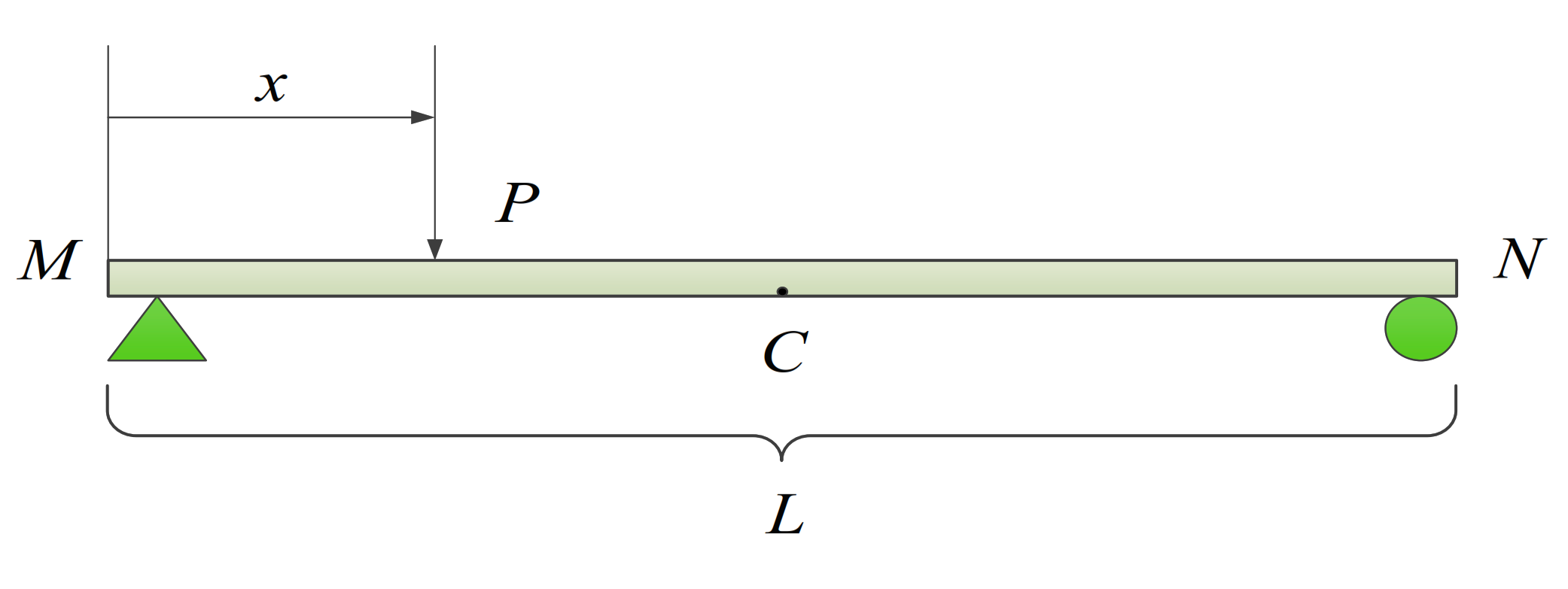
2.1. Identification Theory of Influence Lines

According to the strain influence line theory [28] and material mechanics for a simply supported beam, as shown in Figure 1, the strain of the mid-span point C can be expressed as below:

$${\epsilon }_c=\left\{\begin{array}{c}\frac{Phx}{2EI}\\ \frac{PhL}{2EI}\left(1-\frac{x}{L}\right)\end{array}\right.\begin{array}{c}\\ \end{array}\begin{array}{cc}& \\ & \end{array}\begin{array}{c}\\ \end{array}\begin{array}{c}0<x<\frac{L}{2}\\ \frac{L}{2}<x<L\end{array}$$

(1)

where x is the distance between the moving load P and the beam end A, L is the beam span, h is the height of the neutral axis, I is the section inertia moment of point C, and E is the elastic modulus.

Generally, the moving load on the bridge is a multi-axle vehicle load, so the measured strain response can be seen as the superposition of multiple concentrated loads [29]. Figure 2 shows a three-axle vehicle load as a sample. The strain equation of mid-span section under vehicle load can be expressed as below:

$$\epsilon \left(x\right)={\epsilon }_1\left(x-x_1\right)+{\epsilon }_2\left(x-x_2\right)+{\epsilon }_3\left(x-x_3\right)$$

(2)

where x is the distance between the vehicle’s first axis and the left end of the bridge, x₁, x₂, and x₃ are the distances between each axle and the first axle, P₁, P₂, and P₃ are the axle loads, respectively.

From the above case of three-axle vehicle, the strain response of the mid-span beam under the n-axle vehicle load can be expressed as below:

$$\epsilon \left(x\right)={\displaystyle \sum _{i=1}^n{\epsilon }_n\left(x-x_n\right)}$$

(3)

By introducing Equation (3) into Equation (1), the following equation can be obtained:

$${\epsilon }_n\left(x-x_n\right)=P_{n}f\left(x-x_n\right)$$

(4)

in which:

$$f\left(x\right)=\left\{\begin{array}{c}\frac{hx}{2EI}\\ \frac{hL}{2EI}\left(1-\frac{x}{L}\right)\end{array}\right.\begin{array}{cc}& \\ & \end{array}\begin{array}{c}0<x<\frac{L}{2}\\ \frac{L}{2}<x<L\end{array}$$

(5)

When the multi-axle vehicle passes through the bridge, the area enclosed by the mid-span strain function and the x axis can be expressed as:

$$A={\displaystyle {\int }_{-\infty }^{+\infty }\epsilon \left(x\right)dx}$$

(6)

By introducing Equation (3) into Equation (6), the following equation can be obtained:

$$A={\displaystyle {\int }_{-\infty }^{+\infty }{\displaystyle \sum _{i=1}^n{P}_{n}f\left(x-x_n\right)}dx}={\displaystyle \sum _{i=1}^n{P}_n}{\displaystyle {\int }_{-\infty }^{+\infty }f\left(x-x_n\right)}dx$$

(7)

Consequently, the total weight P of the vehicle can be expressed as:

$$P={\displaystyle \sum _{i=1}^n{P}_n}=\frac{A}{{\displaystyle {\int }_{-\infty }^{+\infty }f\left(x-x_n\right)}dx}=\frac{A}{\alpha }$$

(8)

in which:

$$\alpha ={\displaystyle {\int }_{-\infty }^{+\infty }f\left(x-x_n\right)}dx$$

(9)

where α is the mid-span strain integral coefficient, it is related to the envelope area of the strain influence line. The α can be calibrated by Equation (9) when a known vehicle load passes through the bridge. Then, the α can be used to identify the vehicle load.

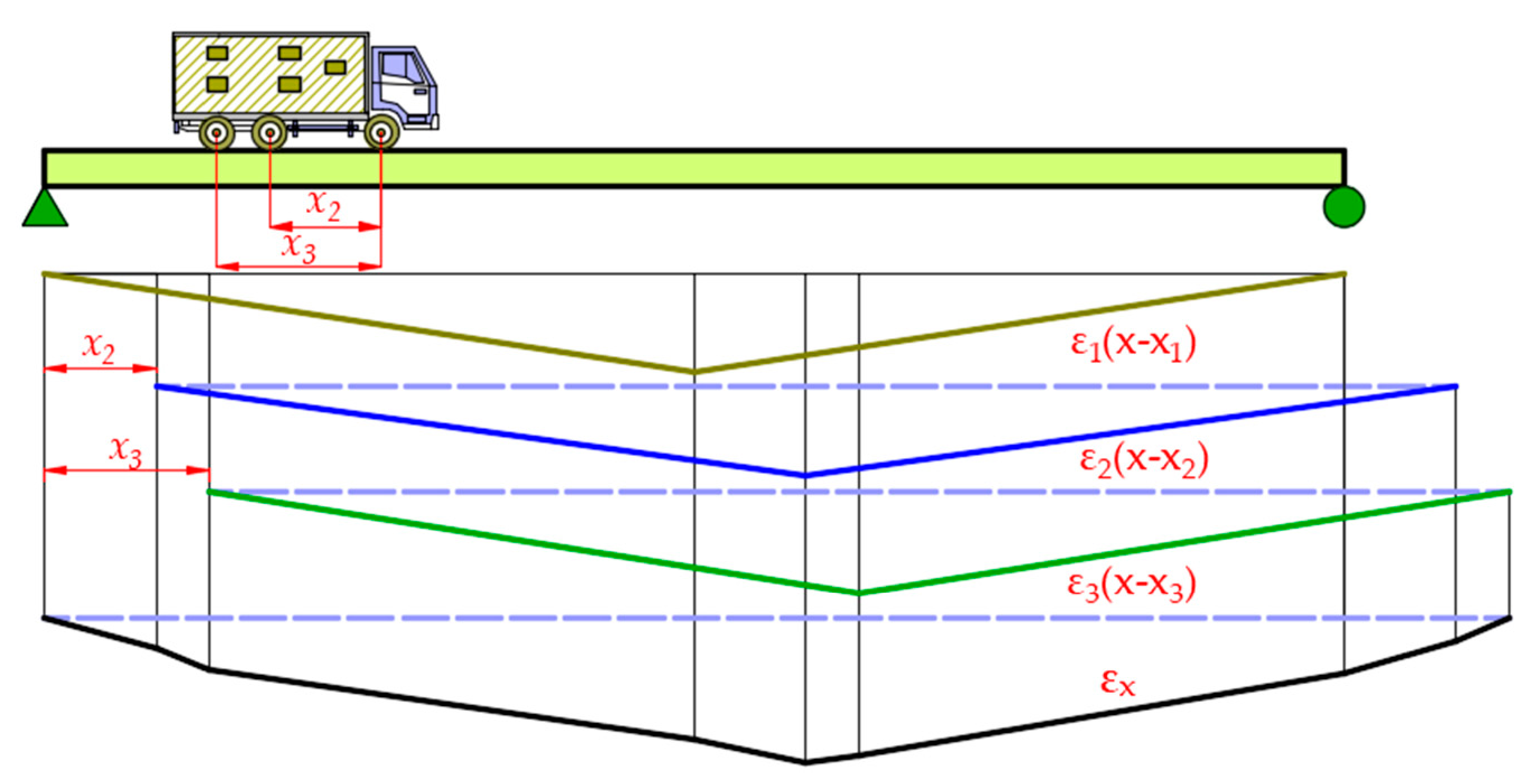
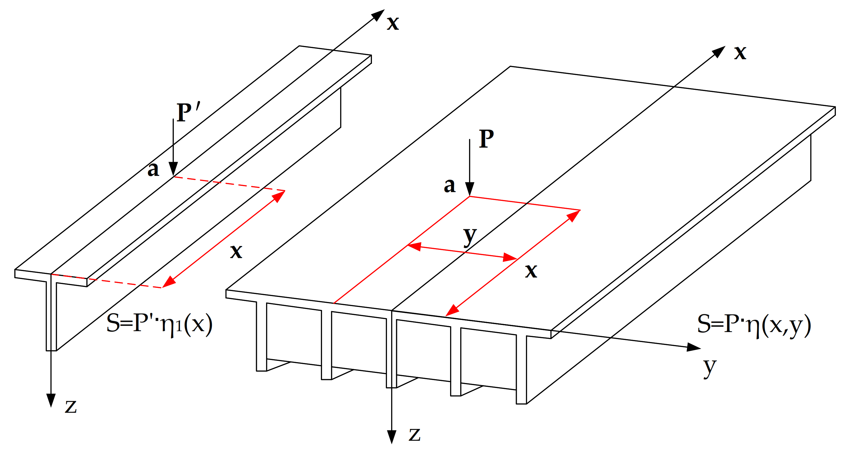
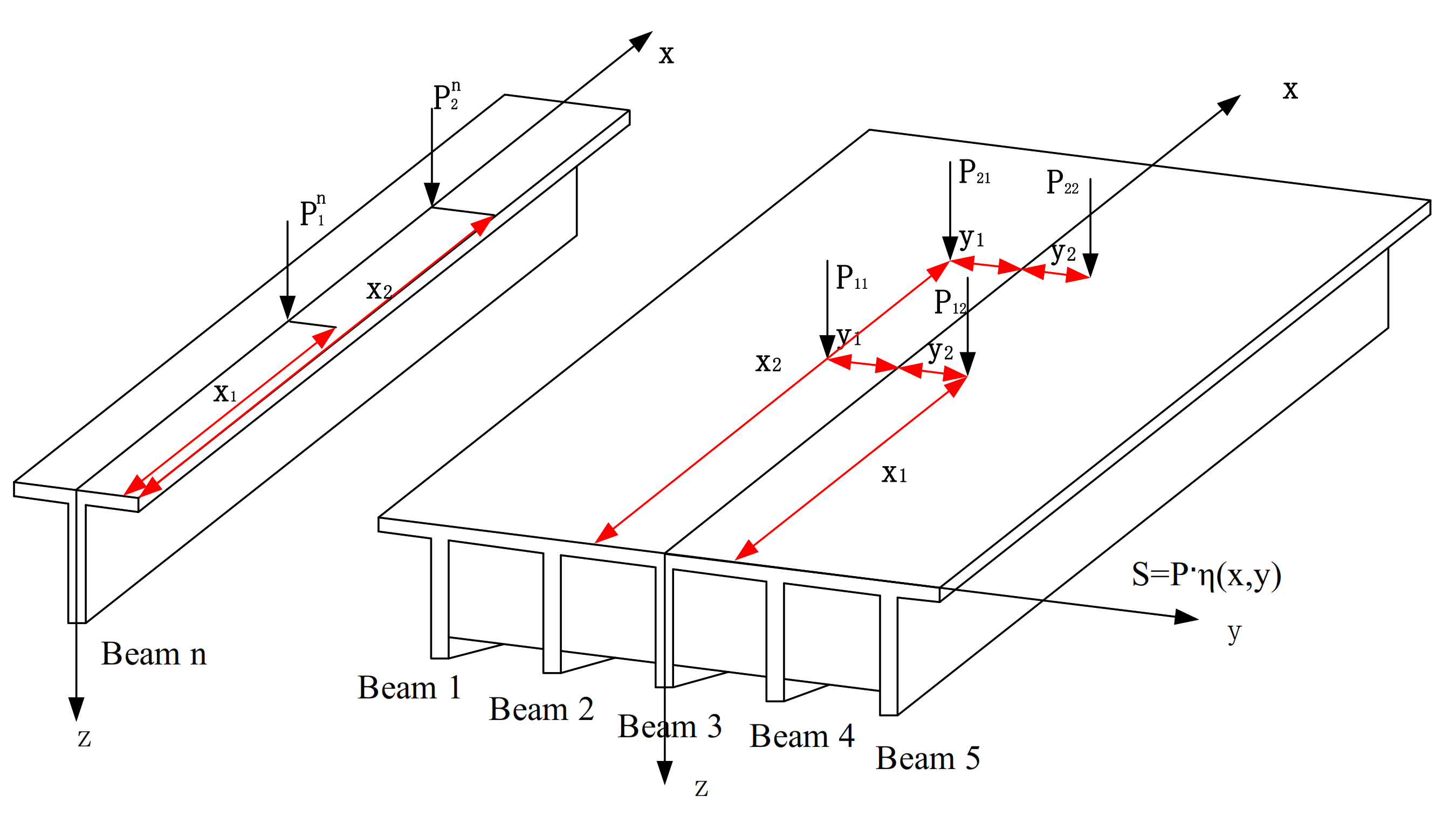
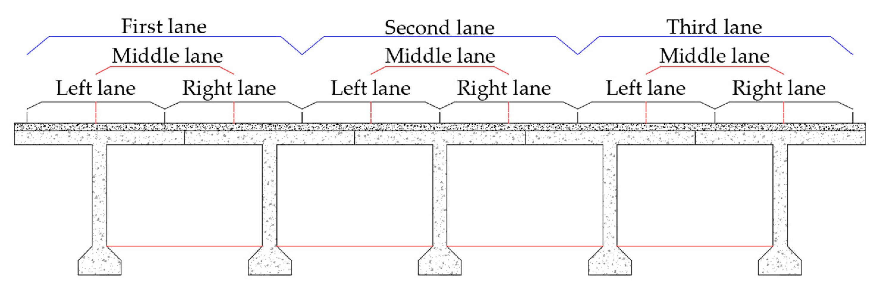
2.2. Moving Load Identification Method Considering the Load Transverse Distribution

When the vehicle load acts on the bridge, the load is not only transmitted in the longitudinal direction, but also in the horizontal direction. Therefore, the force analysis of the bridge under the vehicle load is a space calculation problem. Then, the internal force analysis of the bridge section can be carried out through the influence surface. The influence surface of the bridge internal force can be expressed by a two-valued function η(x, y), then the internal force value of section a can be expressed as $S=P\cdot \eta \left(x,y\right)$, in which S is the internal force value of the section, and P is the vehicle load. In addition, η(x, y) can be separated into the product of two single-valued functions by the separation variable method. That is $\eta \left(x,y\right)={\eta }_1\left(x\right)·{\eta }_2\left(y\right)$, in which η₁(x) is the internal force influence line of the beam section, and η₂(y) is the change curve of the load ratio when the unit load acts in different positions along the horizontal direction. Then, the internal force value P’ of the beam section can be expressed as $P^{\prime }=P\cdot {\eta }_2\left(y\right)$, equivalent to assigned the load to the beam along the horizontal direction when the load P acts on point $a\left(x,y\right)$.

For the simply supported T-beam bridge, as shown in Figure 3, it is approximately assumed that $S=P\cdot \eta \left(x,y\right)\approx P\cdot {\eta }_1\left(x\right)\cdot {\eta }_2\left(y\right)$, which neglects the spatial effect of the bridge and turns it into a plane problem. When a moving load acts on the bridge deck and its position changes with the x coordinate but y coordinate is constant, then the $P\cdot {\eta }_2\left(y\right)$ is constant too. That is the direction of the load transverse distribution coefficient along the beam span does not change. Therefore, each beam can be analyzed individually when analyzing the internal force influence line of the beam section, and the equivalent load of each beam can be obtained according to the load transverse distribution coefficient.

Take the two-axle vehicle as an example to analyze the internal force (as shown in Figure 4). The axle weight is P₁₁, P₁₂, P_21, and P_22, respectively, and its action position is (x₁, y₁), (x₁, y₂), (x₂, y₁), (x₂, y₂), respectively. The y coordinate values of the four wheel loads are constant when the vehicle travels parallel to the x coordinate on the bridge, that is, the transverse distribution coefficient of each wheel load is constant. When analyzing the internal force of a single beam, the equivalent load $\left(P_1^n,P_2^n\right)$ acting on it can be obtained by the following equation:

$$\left\{\begin{array}{c}{P}_1^n=P_{11}\cdot {\eta }_2\left(y_1\right)+P_{12}\cdot {\eta }_2\left(y_2\right)\\ P_2^n=P_{21}\cdot {\eta }_2\left(y_1\right)+P_{22}\cdot {\eta }_2\left(y_2\right)\end{array}\right.\begin{array}{c}\left(n=1,2,3,4,5\right)\end{array}$$

(10)

The total weight of the vehicle can be expressed as:

$$P=P_{11}+P_{12}+P_{21}+P_{22}={\displaystyle \sum _{n=1}^5\left(P_1^n+P_2^n\right)}$$

(11)

According to the influence line theory, when the strain integral coefficient of one beam section is known, the total weight of the moving load can be calculated through the monitored strain integral value on the section.

Assuming that the above vehicle loads drive parallel to the x coordinate from one end to the other end of the beam, the measured strain integral values of the mid-span section of each beam bottom are A₂, A₃, A₄ and A₅, respectively. In addition, it is assumed that the mid-span strain integral coefficients of each beam bottom are α₁, α₂, α₃, α_4, and α₅, respectively. The following equation can be obtained:

$$P={\displaystyle \sum _{n=1}^5\left(P_1^n+P_2^n\right)}={\displaystyle \sum _{n=1}^5\frac{A_n}{{\alpha }_n}}$$

(12)

From Equation (12), it can be seen that the mid-span strain integral coefficient of each beam bottom must be obtained first in order to get the total weight P of the vehicle. The P, A₁, A₂, A₃, A₄, and A₅ in Equation (12) can be obtained by test. Therefore, the essence of calculating the strain integral coefficient is to solve a five-element linear equation. Keeping the vehicle weight constant but changing the driving position (five different values of y₁ and y₂), the equation group can be obtained as below:

$$\left\{\begin{array}{l}\frac{A_{11}}{{\alpha }_1}+\frac{A_{12}}{{\alpha }_2}+\frac{A_{13}}{{\alpha }_3}+\frac{A_{14}}{{\alpha }_4}+\frac{A_{15}}{{\alpha }_5}=P\\ \frac{A_{21}}{{\alpha }_1}+\frac{A_{22}}{{\alpha }_2}+\frac{A_{23}}{{\alpha }_3}+\frac{A_{24}}{{\alpha }_4}+\frac{A_{25}}{{\alpha }_5}=P\\ \frac{A_{31}}{{\alpha }_1}+\frac{A_{32}}{{\alpha }_2}+\frac{A_{33}}{{\alpha }_3}+\frac{A_{34}}{{\alpha }_4}+\frac{A_{35}}{{\alpha }_5}=P\\ \frac{A_{41}}{{\alpha }_1}+\frac{A_{42}}{{\alpha }_2}+\frac{A_{43}}{{\alpha }_3}+\frac{A_{44}}{{\alpha }_4}+\frac{A_{45}}{{\alpha }_5}=P\\ \frac{A_{51}}{{\alpha }_1}+\frac{A_{52}}{{\alpha }_2}+\frac{A_{53}}{{\alpha }_3}+\frac{A_{54}}{{\alpha }_4}+\frac{A_{55}}{{\alpha }_5}=P\end{array}\right.$$

(13)

In order to obtain the strain integral coefficient, its reciprocal can be calculated first:

$$\left\{\frac{\mathbf{1}}{\mathit{\alpha }}\right\}={\left\{\mathit{A}\right\}}^{-\mathbf{1}}\left\{\mathit{P}\right\}$$

(14)

After obtaining the strain integral coefficient by the above method, the vehicle load identification can be carried out subsequently. Moreover, it should be noted that the theoretical derivation above is aimed at the simply supported T-beam bridge, but the method is still applicable to the similar bridge types, such as box girder bridges.

3. Numerical Simulation

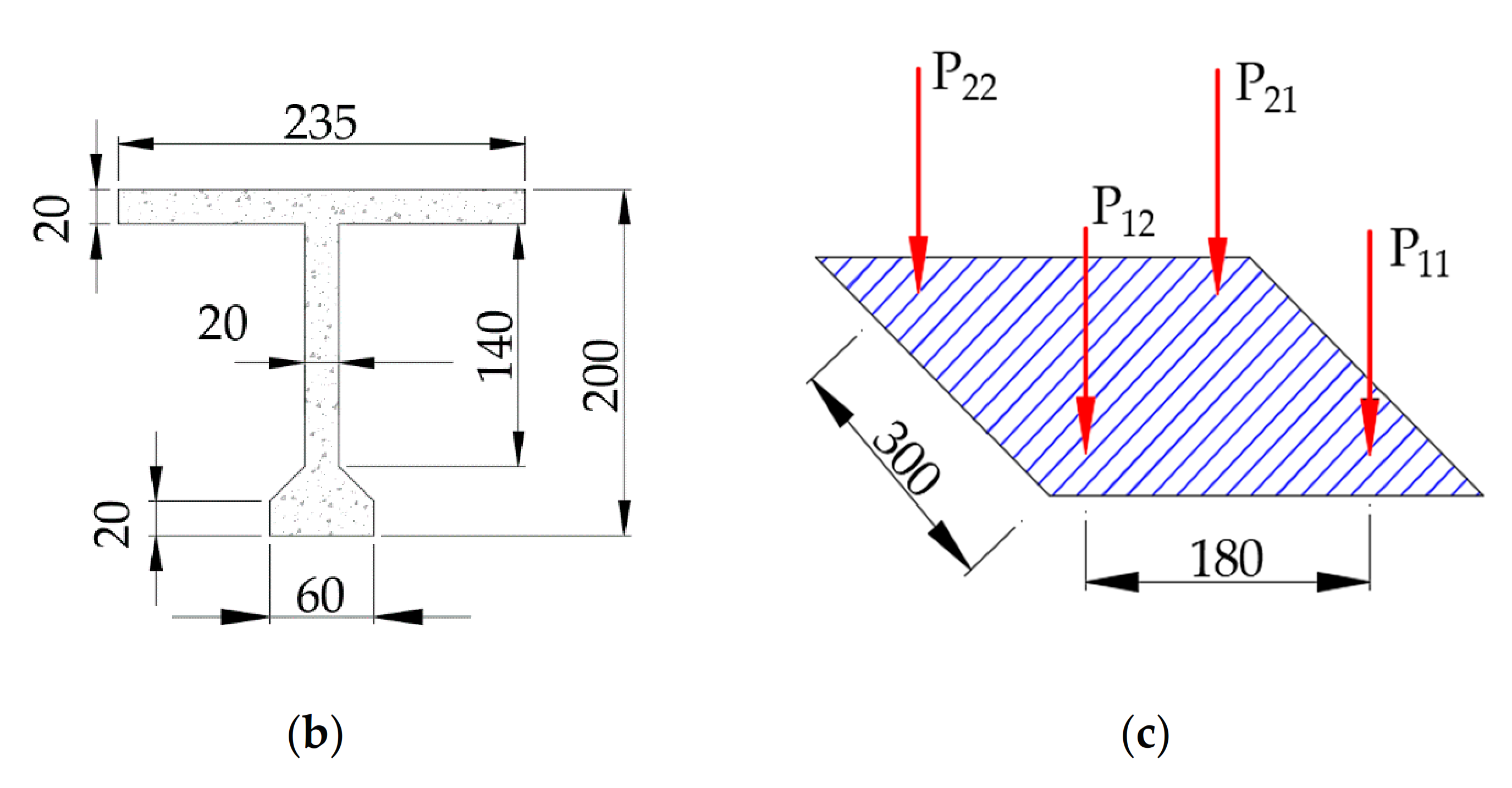
3.1. Model Building

In order to verify the effectiveness of the above method, a numerical analysis model of T-beam bridge was established, as shown in Figure 5, the model beam is 3 m in length, 1.175 m in width, 0.21 m in height, the section size is shown in Figure 5a,b. The density of the mode material is 1170 kg/m³, the Poisson’s ratio is 0.35. The elastic modulus of 1# beam is E₁ = 3.25 × 10⁴ MPa, and the elastic modulus of 2#~5# beams are E₂ = 1.02 E₁, E₃ = 1.05 E₁, E₄ = 1.07 E₁, E₅ = 1.1 E₁, respectively.

Assuming that the vehicle load acting on the bridge was represented by four time-varying forces, its equation can be expressed as below:

$$\left\{\begin{array}{l}{P}_{11}=P_{12}=P\left(0.2+0.025\sin \left(6.67\pi t\right)\right)\\ P_{21}=P_{22}=P\left(0.3+0.025\sin \left(6.67\pi t\right)\right)\end{array}\right.$$

(15)

where, P₁₁ and P₁₂ represented the front wheel loads, P₂₁ and P₂₂ represented the rear wheel loads, P was the total weight of the vehicle. The vehicle wheelbase was 300 mm, the wheel-track was 180 mm, and the vehicle speed was 1 m/s, as shown in Figure 5c.

The vehicle load P was divided into three grades, 10 kg, 20 kg, and 30 kg, respectively. The load grade of 10 kg was used to calibrate the strain integral coefficient, and the other load grades were used to test. As shown in Figure 6, the bridge model was divided into three lanes, and the vehicle acted on the left, middle, and right positions of each lane. Thus, the vehicle load position was divided into nine conditions.

3.2. Simulation Results Analysis

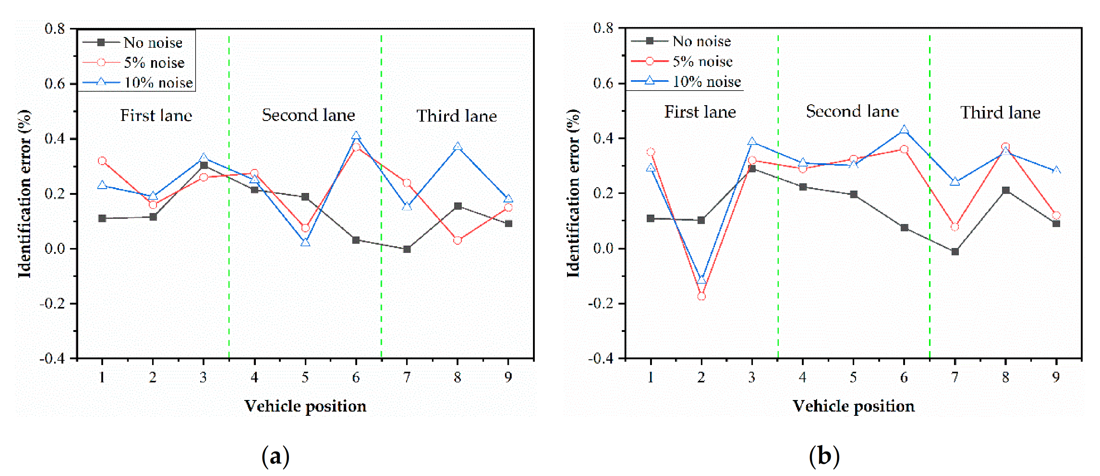
3.2.1. Analysis of the Identification Results without Considering the Load Transverse Distribution

For the identification method without considering the load transverse distribution, it is only necessary to know the mid-span strain integral coefficient α of a single beam. Firstly, the following simulation conditions were carried out: (1) Vehicle driving in the middle of the first lane with 10 kg weight at 1 m/s, (2) vehicle driving in the middle of the second lane with 10 kg weight at 1m/s, (3) vehicle driving in the middle of the third lane with 10 kg weight at 1m/s. According to each working conditions, the corresponding mid-span strain influence line (1#, 3#, 5# beam) were obtained, as shown in Figure 7, then the corresponding strain integral coefficient was obtained in

Table 1. The strain integral coefficient.

Vehicle Driving Position	The Middle of the First Lane	The Middle of the Second Lane	The Middle of the Third Lane
Beam number	1#	3#	5#
Total weight (kg)	10	10	10
The integral value of strain influence line (10−6 m)	14.46	7.57	13.48
Strain integral coefficient (10−8)	14.75	7.73	13.75

.

Figure 8 shows the load identification results obtained according to the strain integral coefficient. Taking the strain integral coefficient of 3# beam as an example, it can be seen that the identification error was smaller than 10% when the vehicle load drove in the second lane. Especially when the vehicle load drove in the middle of the second lane, the error was almost zero. However, the identification error was large when the vehicle drove in the first and third lane. Therefore, it was not suitable for load identification. For the load identification results obtained according to the strain integral coefficient of 1# beam and 5# beam, the identification error was close to zero when the vehicle load drove in the middle of the first and third lane. However, the identification accuracy was still poor when the vehicle load drove in the left or the right line. In addition, the farther away from the vehicle position of coefficient calibration, the worse the identification accuracy was. In summary, the load identification accuracy was closely related to the driving position of the vehicle load when the influence of load transverse distribution was not considered. The identification accuracy was relatively high when it was close to the vehicle position of coefficient calibration, conversely, the identification accuracy was poor. Therefore, it was no longer suitable for load identification.

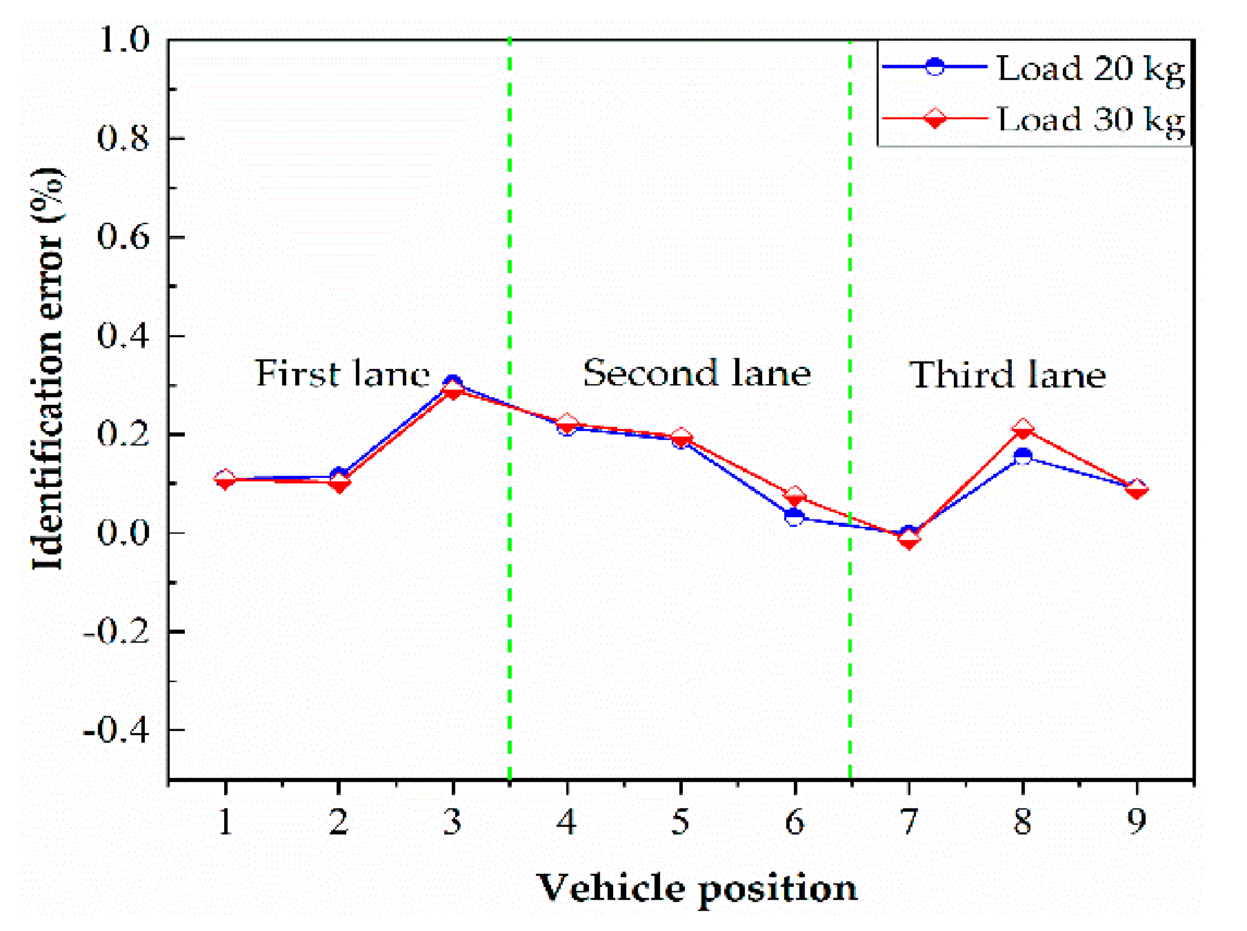
3.2.2. Analysis of the Identification Results Considering the Load Transverse Distribution

For the identification method considering the load transverse distribution, it was necessary to obtain the strain integral coefficient of each beam by Equation (14). Firstly, the following simulation conditions were carried out with the vehicle load of 10 kg: (1) Vehicle driving in the left of the first lane, (2) vehicle driving in the right of the first lane, (3) vehicle driving in the middle of the second lane, (4) vehicle driving in the left of the third lane, (5) vehicle driving in the right of the third lane. According to Equations (13) and (14), the strain integral coefficient of each beam was obtained (as shown in

Table 2. The mid-span strain integral coefficient of each beam bottom.

	1# Beam	2# Beam	3# Beam	4# Beam	5# Beam
Strain integral coefficient (10−8)	29.17	28.84	27.93	27.70	26.61
Ratio to integral coefficient of 1# beam	1	0.989	0.957	0.949	0.912
Ratio to reciprocal 1# beam stiffness	1	0.980	0.952	0.936	0.910

). It can be seen that the strain integral coefficient of each beam bottom was basically proportional to the reciprocal of the stiffness, and the reason for the error was that the load identification method considering the load transverse distribution, which ignores the influence of spatial effect and diaphragm in the theoretical derivation. The obtained strain integral coefficient was used to identify the load of the test sample, and the results are shown in Figure 9. It can be seen that the identification accuracy was very high no matter where the vehicle was, and the error was close to zero. Therefore, compared with the identification method without considering the load transverse distribution, the identification method considering the load transverse distribution has obvious advantages.

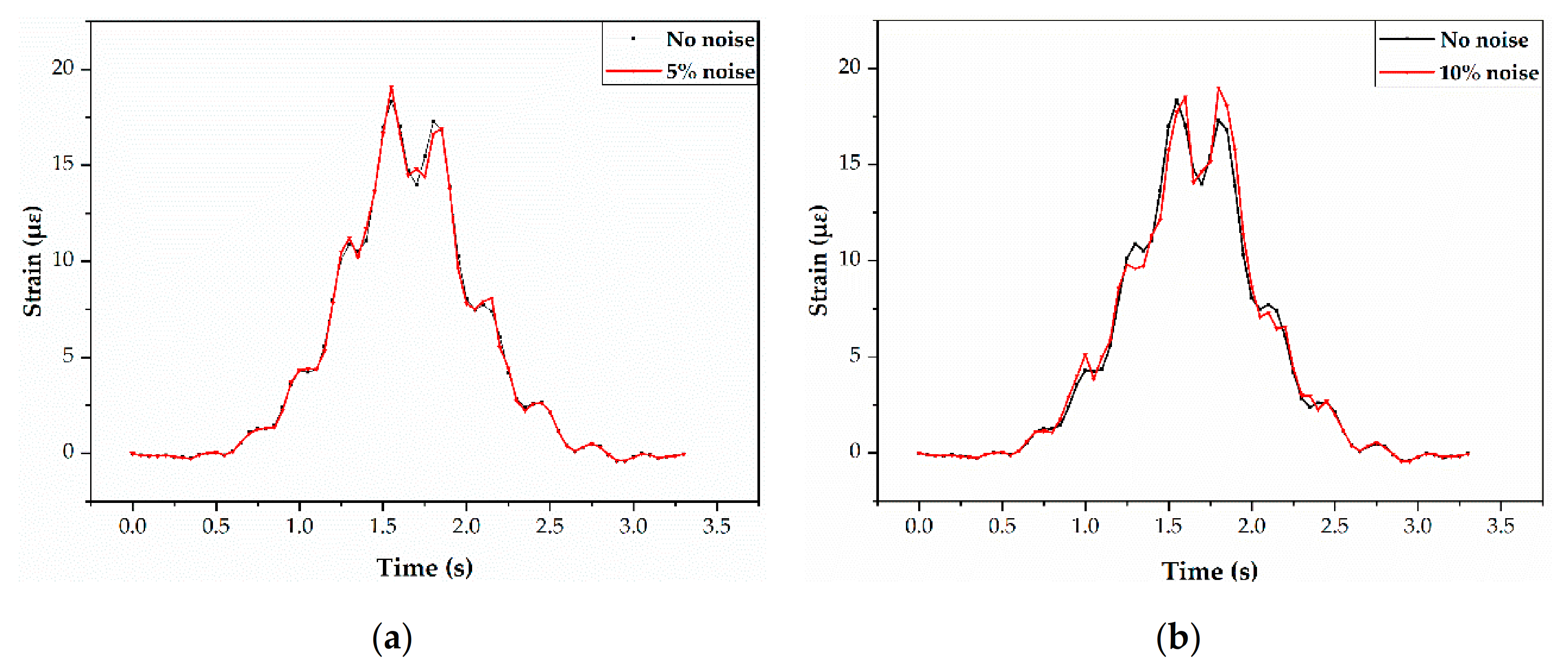
3.2.3. Analysis of the Anti-Noise Performance

Two kinds of noise (5% and 10%) were added to the numerical simulation to verify the anti-noise performance of the method. The strain values of the test sample were extracted, and 5% and 10% of the noise were added as condition 1 and condition 2, and the noise can be expressed as:

$${\epsilon }^{\prime }(x)=\epsilon (x)+\beta ·rand(n)·var(x)$$

(16)

where ε’(x) is the strain output after the added noise, ε(x) is the original strain input, β is the noise level, rand is short for random and rand(n) is a set of values with the mean is 0 and the variance is 1, var is short for variance and var(x) is the variance of the original strain input.

When the vehicle load (20 kg) drives in the middle of the second lane, the mid-span strain time history with different kinds of noise of 3# beam bottom is shown in Figure 10. It can be seen that there is only a slight fluctuation of the strain output when the noise level is 5%, which can better simulate the environmental noise. The strain output has an obvious difference for the original value when the noise level reaches 10%, both of these two working conditions are representative. The load identification results with different levels of noise are shown in Figure 11. It can be seen that the load identification error with different noise levels was slightly larger compared with the no-noise condition. The load identification errors were nearly the same when the noise levels were 5% and 10%. In addition, the overall error was smaller than 0.5%, which showed a good identification accuracy. Therefore, the method can keep the identification accuracy under different kinds of noise, and the noise reduction for the following analysis processing can be ignored.

4. Verification by Experiment

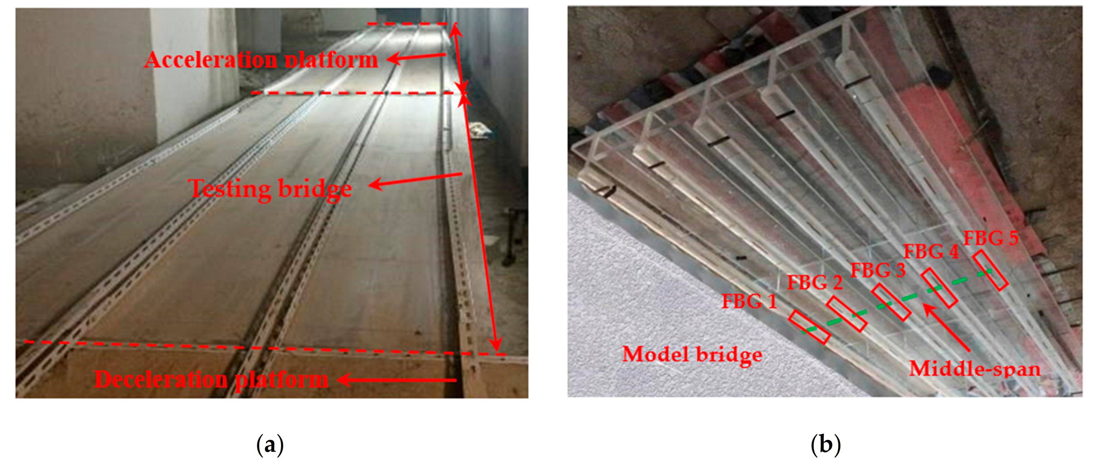
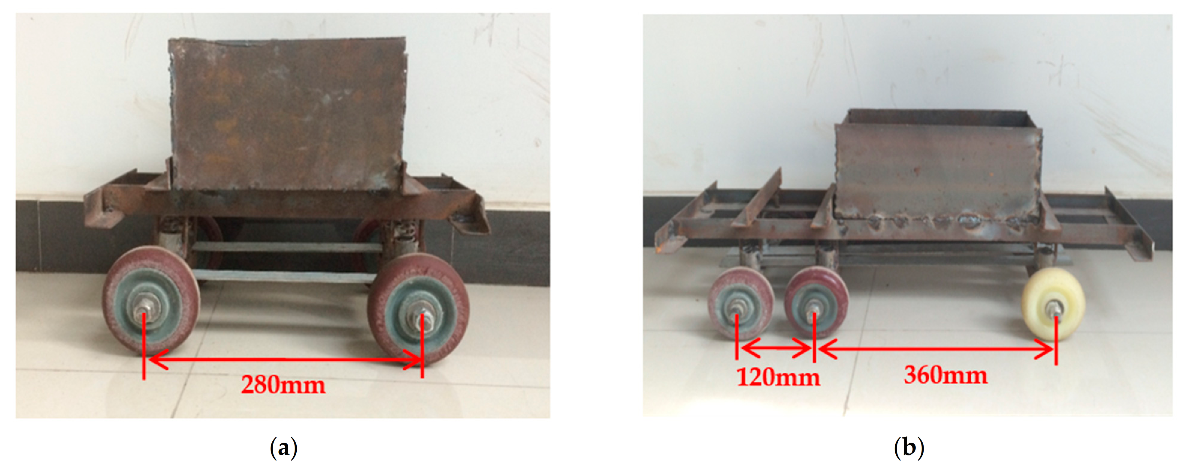
4.1. Experimental Setup

To test the feasibility of the proposed method, a series of bridge model experiments were conducted. The experimental platform was made of an acceleration platform, test bridge, and deceleration platform, which is shown in Figure 12a. The model bridge was made according to the size of the numerical simulation bridge, as shown in Figure 5, the material of the model bridge is polymethyl methacrylate (as shown in Figure 12b), and its density is 1170 kg/m³, the Poisson’s ratio is 0.35, and the elastic modulus is 3.25 × 10⁴ MPa.

The experimental vehicle models were divided into two-axle and three-axle vehicles, as shown in Figure 13, and the way to change the vehicle weight was to add counterweight in the vehicle. In addition, the long-gauge FBG strain sensors were used to collect and analyze the data in the experiment [1]. Based on the influence line method considering the load transverse distribution, five FBG strain sensors were arranged in the mid-span of each beam bottom, as shown in Figure 12b.

4.2. Analysis of Experiment Results

The MOI’s S130 model acquisition instrument was used to collect the data of FBG sensors in the experiment, and the measured data were used for load identification. When the vehicle drives in the second lane with the speed of 1.33 m/s, the typical long-gauge strain time history curve of each beam bottom is shown in Figure 14.

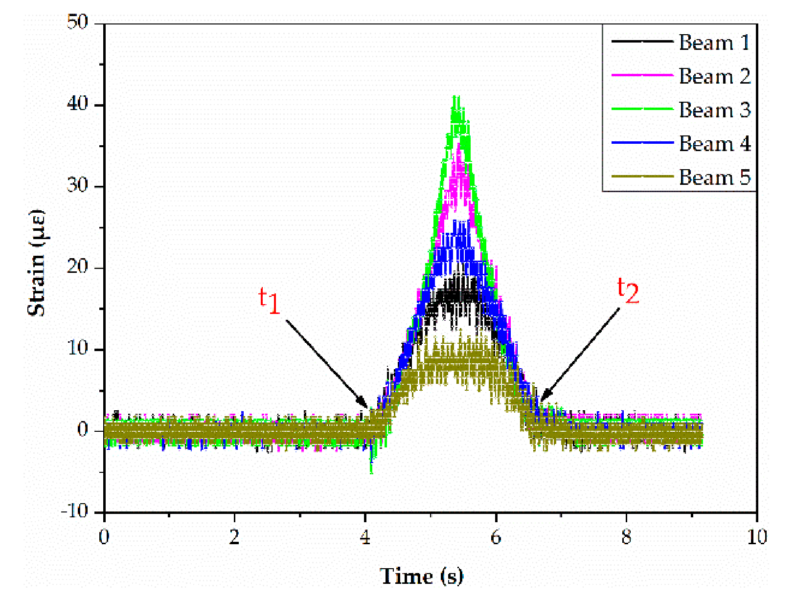
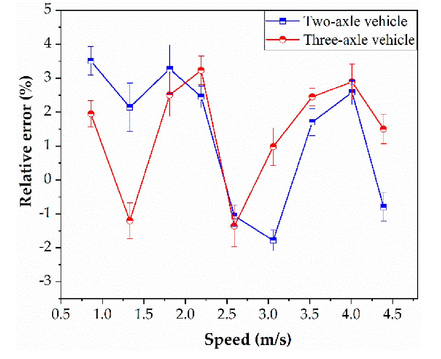
4.2.1. Speed Identification

Firstly, the vehicle speed was identified. Assuming that the vehicle crosses the bridge with a constant speed, the integral Equation (17) of strain influence line can be obtained by modifying Equation (6):

$$A={\displaystyle {\int }_{-\infty }^{+\infty }\epsilon \left(x\right)dx}={\displaystyle {\int }_{-\infty }^{+\infty }\epsilon \left(t\right)vdt}=v{\displaystyle {\int }_{-\infty }^{+\infty }\epsilon \left(t\right)dt}$$

(17)

As shown in Figure 14, it corresponds to the starting point t₁ of the wave peak when the front axle of the vehicle contacts the bridge, and it corresponds to the ending point t₂ when the rear axle of the vehicle leaves the bridge. Then the vehicle speed V can be calculated according to the time difference and the driving distance, as shown in Equation (18):

$$v=\frac{d}{\Delta t}=\frac{L+x}{t_2-t_1}$$

(18)

where, x is the vehicle wheelbase, L is the bridge length. In this experiment, the vehicle weight was 16.95 kg, and the vehicle speed was divided into nine levels by changing the speed of traction motor, as shown in

Table 3. Speed levels.

Vehicle Speed (m/s)

0.86

1.33

1.81

2.19

2.59

3.06

3.53

4.01

4.39

. Meanwhile, each experimental condition was repeated three times. According to the above method, the strain data of 3# beam bottom were used to identify the vehicle speed, and the results are shown in Figure 15. It can be seen that the average relative errors of the speed identification were smaller than ±4%, and they were within an acceptable range, which shows the great performance of the method.

4.2.2. Influence of Speed on Load Identification

Based on the vehicle speed obtained from inversion, the strain time history curve was converted into strain influence line. Then, the load identification was carried out by the method considering the load transverse distribution. The samples with the weight of 28 kg and speed of 0.86 m/s were selected to calibrate the strain integral coefficient. It should be noted that the driving path of the vehicle was limited to three lanes, so the five equations that were shown in Equation (13) cannot be obtained. However, the optimal solution of the strain integral coefficient can be obtained by using three equations, as shown in

Table 4. The mid-span strain integral coefficient of each beam bottom.

	1# Beam	2# Beam	3# Beam	4# Beam	5# Beam
The strain integral coefficient (10−7)	8.11	8.33	8.04	7.23	7.08

.

According to Equation (17), the integral value of the influence line is independent of the vehicle speed, but the identification accuracy of the speed has an effect on the integral value. The actual speed and inversion speed were used to identify the vehicle weight of the above 18 samples, which was mentioned in Section 4.2.1, and the results are shown in Figure 16. It can be seen that the speed had no obvious influence on vehicle weight identification, and the average identification error was smaller than ±5%. In addition, it should be noted that the results obtained by using the actual speed to calculate the vehicle weight were more accurate than those obtained by using the inversion speed. Moreover, the average identification error was smaller than 2% when using the actual speed to identify the vehicle weight.

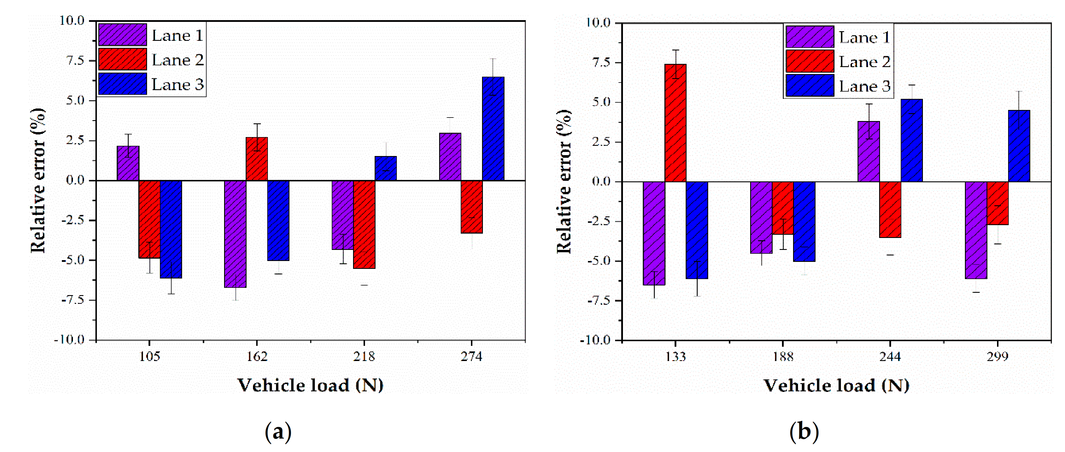
4.2.3. The Identification Results of Vehicle Weight

As the vehicle speed has no obvious influence on the identification results of the vehicle weight, the vehicle speed was set as 1.33 m/s in the following analysis. The two-axle vehicle and three-axle vehicle were divided into four grades of weight in the experiment. Each grade of vehicle weight was tested in three lanes, and the load identification results were shown in Figure 17. It can be seen that no matter which lane the vehicle drives, the vehicle weight identification error of each sample can be controlled within ±10%. The error of more than 90% of samples was smaller than ±5%, and the error was relatively larger compared with the simulation results, which was within an acceptable range. In addition, the error fluctuation of load identification was small, and the variance was smaller than 2%. Compared with reference [26], the method proposed in this paper greatly improves the identification accuracy. Therefore, it can be considered that the load identification method considering the load transverse distribution was effective. The error sources should be analyzed in the following aspects: (1) The vehicle weight identification is based on the speed identification, so the error of vehicle speed will affect the result of vehicle weight identification, (2) although there are lane restrictions in the experiment, the vehicle’s trajectory is not always in a straight line along the bridge span direction, and its trajectory is relatively random.

5. Conclusions

In this paper, considering the load transverse distribution, a novel moving load identification method was proposed based on distributed strain sensing technique and influence line. The load identification accuracy and anti-noise performance were greatly improved, and it was more universal for a variety of bridge types. In addition, a series of numerical simulations and experiments were conducted to verify the proposed method. The main conclusions are as follows:

• Through the verification of numerical simulation, the method without considering the load transverse distribution was not suitable for solving the space problem, and the method considering the load transverse distribution has a high identification accuracy and excellent performance of anti-noise performance.
• The results of the model test showed that the average relative error of the speed identification was smaller than ±4%, which shows the great performance of the method.
• The speed has no obvious influence on the vehicle weight identification, and the average identification error was smaller than ±5%. In addition, it should be noted that the results obtained by using the actual speed to calculate the vehicle weight were more accurate than those obtained by using the inversion speed.
• The relative error of the vehicle weight identification was smaller than ±10%, and the error of more than 90% of samples was smaller than ±5%.

References

1. Li, S.Z.; Wu, Z.S. Development of distributed long-gage fiber optic sensing system for structural health monitoring. Struct. Health Monit. 2007, 6, 133–143. [Google Scholar] [CrossRef]
2. Cardini, A.J.; DeWolf, J.T. Long-term structural health monitoring of a multi-girder steel composite bridge using strain data. Struct. Health Monit. 2009, 8, 47–58. [Google Scholar] [CrossRef]
3. Brownjohn, J.M.W. Structural health monitoring of civil infrastructure. Philos. Trans. R. Soc. Lond. Ser. A 2007, 365, 589–622. [Google Scholar] [CrossRef] [PubMed] [Green Version]
4. Wong, K.Y. Instrumentation and health monitoring of cable-supported bridges. Struct. Control Health Monit. 2004, 11, 91–124. [Google Scholar] [CrossRef]
5. Li, H.N.; Li, D.S.; Song, G.B. Recent applications of fiber optic sensors to health monitoring in civil engineering. Eng. Struct. 2004, 26, 1647–1657. [Google Scholar] [CrossRef]
6. Karoumi, R.; Wiberg, J.; Liljencrantz, A. Monitoring traffic loads and dynamic effects using an instrumented railway bridge. Eng. Struct. 2005, 27, 1813–1819. [Google Scholar] [CrossRef]
7. Sekuła, K.; Kołakowski, P. Piezo-based weigh-in-motion system for the railway transport. Struct. Control Health Monit. 2012, 19, 199–215. [Google Scholar] [CrossRef]
8. Kim, S.H.; Heo, W.H.; You, D. Vehicle loads for assessing the required load capacity considering the traffic environment. Appl. Sci. 2017, 7, 365. [Google Scholar] [CrossRef] [Green Version]
9. Kim, S.H.; Choi, J.G.; Ham, S.M. Reliability evaluation of a PSC highway bridge based on resistance capacity degradation due to a corrosive environment. Appl. Sci. 2016, 6, 423. [Google Scholar] [CrossRef] [Green Version]
10. Ghosh, J.; Caprani, C.C.; Padgett, J.E. Influence of traffic loading on the seismic reliability assessment of highway bridge structures. J. Bridge. Eng. 2014, 19, 04013009. [Google Scholar] [CrossRef]
11. Pinkaew, T. Identification of vehicle axle loads from bridge responses using updated static component technique. Eng. Struct. 2006, 28, 1599–1608. [Google Scholar] [CrossRef]
12. Han, L.D.; Ko, S.S.; Gu, Z.; Jeong, M.K. Adaptive weigh-inmotion algorithms for truck weight enforcement. Transp. Res. 2012, 24, 256–269. [Google Scholar]
13. Richardson, J.; Jones, S.; Brown, A.; O’Brien, E.; Hajialzadeh, D. On the use of bridge weigh-in-motion for overweight truck enforcement. Int. J. Heavy Veh. Syst. 2014, 21, 83–104. [Google Scholar] [CrossRef]
14. Yu, Y.; Cai, C.S.; Deng, L. State-of-the-art review on bridge weigh-in-motion technology. Adv. Struct. Eng. 2016, 19, 1514–1530. [Google Scholar] [CrossRef]
15. Bajwa, R.; Coleri, E.; Rajagopal, R.; Varaiya, P.; Flores, C. Development of a cost-effective wireless vibration weigh-in-motion system to estimate axle weights of trucks. Comput. Aided Civ. Inf. Eng. 2017, 32, 443–457. [Google Scholar] [CrossRef]
16. Zolghadri, N.; Halling, M.; Johnson, N.; Barr, P. Field verification of simplified bridge weigh-in-motion techniques. J. Bridge. Eng. 2016, 21, 04016063. [Google Scholar] [CrossRef]
17. Ojio, T.; Carey, C.; Obrien, E.; Doherty, C.; Taylor, S.E. Contactless bridge weigh-in-motion. J. Bridge. Eng. 2016, 21, 04016032. [Google Scholar] [CrossRef] [Green Version]
18. Zhao, H.; Uddin, N.; O’Brien, E.; Hao, X.S.; Zhu, P. Identification of vehicular axle weights with a bridge weigh-in-motion system considering transverse distribution of wheel loads. J. Bridge. Eng. 2014, 19, 04013008. [Google Scholar] [CrossRef] [Green Version]
19. Helmi, K.; Taylor, T.; Ansari, F. Shear force based method and application for real-time monitoring of moving vehicle weights on bridges. J. Intell. Mater. Syst. Struct. 2015, 26, 505–516. [Google Scholar] [CrossRef]
20. Zhu, X.Q.; Law, S.S. Practical aspects in moving load identification. J. Sound Vib. 2002, 258, 123–146. [Google Scholar] [CrossRef]
21. Yang, H.; Yan, W.; He, H. Parameters Identification of Moving Load Using ANN and Dynamic Strain. Shock Vib. 2016, 2016, 1–13. [Google Scholar] [CrossRef]
22. Wang, Y.; Qu, W.L. Moving train loads identification on a continuous steel truss girder by using dynamic displacement influence line method. Int. J. Steel Struct. 2011, 11, 109–115. [Google Scholar] [CrossRef]
23. Chen, S.Z.; Wu, G.; Feng, D.C.; Zhang, L. Development of a bridge weigh-in-motion system based on long-gauge fiber Bragg grating sensors. J. Bridge. Eng. 2018, 23, 04018063. [Google Scholar] [CrossRef]
24. Zhang, L.; Wu, G.; Li, H.; Chen, S. Synchronous Identification of Damage and Vehicle Load on Simply Supported Bridges Based on Long-Gauge Fiber Bragg Grating Sensors. J. Perform. Constr. Fac. 2020, 34, 04019097. [Google Scholar] [CrossRef]
25. Wang, H.; Zhu, Q.; Li, J.; Mao, J.; Hu, S.; Zhao, X. Identification of moving train loads on railway bridge based on strain monitoring. Smart Struct. Syst. 2019, 23, 263–278. [Google Scholar]
26. Yang, C.Q.; Yang, D.; He, Y.; Wu, Z.S.; Xia, Y.F.; Zhang, Y.F. Moving load identification of small and medium-sized bridges based on distributed optical fiber sensing. Int. J. Struct. Stab. Dyn. 2016, 16, 1640021. [Google Scholar] [CrossRef]
27. Zuo, X.H.; He, W.Y.; Ren, W.X. Vehicle weight identification for a bridge with multi-T-girders based on load transverse distribution coefficient. Adv. Struct. Eng. 2019, 22, 3435–3443. [Google Scholar] [CrossRef]
28. Ojio, T.; Yamada, K. Bridge weigh-in-motion systems using stringers of plate girder bridges. In Proceedings of the Third International Conference on Weigh-in-Motion (ICWIM3) Iowa State University, Ames, Orlando, FL, USA, 13–15 May 2002. [Google Scholar]
29. O’Connor, C.; Chan, T.H.T. Dynamic wheel loads from bridge strains. J. Struct. Eng. 1988, 114, 1703–1723. [Google Scholar] [CrossRef]
Figure 1. Moving load acting on the simply supported beam.
Applsci 11 00853 g001
Figure 2. Mid-span strain influence line under moving load.
Applsci 11 00853 g002
Figure 3. The internal force calculation under vehicle load.
Applsci 11 00853 g003
Figure 4. Wheel load transverse distribution on the bridge.
Applsci 11 00853 g004
Figure 5. (a) Bridge model, (b) bridge section size, (c) vehicle load (unit: mm).
Applsci 11 00853 g005aApplsci 11 00853 g005b
Figure 6. Vehicle load position.
Applsci 11 00853 g006
Figure 7. The middle-span strain influence line of (a) 1# beam, (b) 3# beam, (c) 5# beam.
Applsci 11 00853 g007
Figure 8. Identification results according to the strain integral coefficient of (a) 1# beam, (b) 3# beam, (c) 5# beam.
Applsci 11 00853 g008
Figure 9. Identification results considering the load transverse distribution.
Applsci 11 00853 g009
Figure 10. The mid-span strain time history of 3# beam with (a) 5% noise, (b) 10% noise.
Applsci 11 00853 g010
Figure 11. Identification error under different levels of noise with the load of: (a) 20 kg, (b) 30 kg.
Applsci 11 00853 g011
Figure 12. (a) Experimental platform, (b) model bridge.
Applsci 11 00853 g012
Figure 13. Vehicle model in the experiment: (a) Two-axle vehicle, (b) three-axle vehicle.
Applsci 11 00853 g013
Figure 14. Measured strain time history curve.
Applsci 11 00853 g014
Figure 15. Relative error of the speed identification.
Applsci 11 00853 g015
Figure 16. Influence of vehicle speed on load identification: (a) Two-axle vehicle, (b) three-axle vehicle.
Applsci 11 00853 g016
Figure 17. The relative error of vehicle weight identification: (a) Two-axle vehicle, (b) three-axle vehicle.
Applsci 11 00853 g017