Abstract
Vehicles driving on the road continuously suffer low-frequency and high-intensity road excitation, which can cause the occupant feelings of tension and dizziness. To solve this problem, a three-degree-of-freedom vehicle suspension system model including vehicle seat is established and a linear function equivalent excitation method is proposed. The optimization of the random excitation is transformed into the optimization of constant force in a discrete time interval, which introduces the adaptive weighted particle swarm optimization algorithm to optimize the delay and feedback gain parameters in the feedback control of time delay. In this paper, the stability switching theory is used for the first time to analyze the stability interval of 3-DOF time-delay controlled active suspension, which ensures the stability of the control system. The numerical simulation results show that the algorithm can reduce vertical passenger acceleration and vehicle acceleration, respectively, by 13.63% and 28.38% on average, and 29.99% and 47.23% on random excitation, compared with active suspension and passive suspension based on inverse control. The effectiveness of the method to suppress road random interference is verified, which provides a theoretical reference for further study of suspension performance optimization with time-delay control.
1. Introduction
The suspension is an important device to ensure the comfort and safety of the ride for the vehicle running on the road [1,2,3,4,5]. This main function is to mitigate the impact and vibration caused by uneven pavement. The road excitation to the vehicle exhibits low-frequency and high-amplitude shock vibration in all directions. Many studies have shown that long-term exposure to low frequency and high-intensity vibration will seriously affect the physical and mental health of passengers. Therefore, research on vibration reduction of vehicle body and seat is of great significance to improve the driving comfort of vehicles and the physical and mental health of occupants [6,7,8].
The active suspension system is modified from the passive suspension in terms of the actuator (motor, hydraulic device, cylinder, etc.). Utilizing a device generating an active force, it can actively suppress the impact of uneven road surfaces on the car body. Therefore, it has obvious advantages in vibration reduction and a wide range of application prospects [9,10]. There are unavoidable time-delay factors in the active suspension system, including the transmission delay of measurement signal from the signal sensor to a controllable computer, the calculation delay caused by calculation control method, the transmission delay of the control signal from the computer to the actuator, the actuator delay, etc. [11,12]. On the one hand, the time delay may lead to the instability of the vibration control system, and the bifurcation phenomenon, which is harmful to safety, will occur and seriously affect the vehicle’s ride comfort. On the other hand, a reasonable design of time delay can improve the control effect of the system. Some studies have been carried out to solve the problem of delay control. Filipovic and Olgac et al. [13,14,15,16] first proposed using time-delay feedback to control the vibration of the main system. Its basic idea is to install a delay-state-feedback shock absorber on the main system. When the external excitation frequency is consistent with the natural frequency of the system, the vibration can be completely eliminated [17,18,19]. Saeed et al. [20,21,22] integral suspended Jeffcott-rotor system is an object of research. They use the time-delay displacement feedback controller to control the lateral motion of the system and analyze the stability of the controller gain and time-delay, which uses simulation analysis to verify the effectiveness of time-delay vibration reduction. Maccari et al. [23] carried out time-delay feedback control for cantilever beams. They use the perturbation method to obtain the appropriate time-delay feedback control parameters, which can reduce the main resonance amplitude and suppress the quasi-period of the beam. Udwadia et al. [24] research on the time-delay problem of active control of torsion bars and building structures shows that introducing the hour delay into the system is helpful to improve the stability and dynamic performance of the system. Zhao and Xu et al. [25,26,27,28] considered time-delay in state feedback control. The time delay and control gain is adjusted to study the delay’s dynamic vibration absorber system. The results show that the vibration of the main system can be almost completely suppressed with appropriate hysteresis control parameters. Chen and Cai [29,30,31,32] et al. designed a flexible manipulator with time-delay feedback control by using numerical simulation and simulation experiments. They found that it had better motion than a flexible manipulator with no time delay. Phu D X et al. [33,34,35,36], to improve the comfort of car seats, proposed a new control strategy to improve ride comfort and applied it to the vibration control of automobile seat suspension with MR damper. The experimental results show the effectiveness of the proposed method.
In general, most of the current research on shock absorbers with time-delay control focuses on the determination of feedback gain of shock absorbers, time-delay parameters, and stability analysis. However, in the research into the control of time-delay vibration reduction under complex excitation, the existing methods of time-delay control parameters do not consider the external excitation in the parameter-solving process. This means that the time-delay parameter is irrelevant to the external excitation. As a result, there are no methods available to solve the time-delay control parameters for different external excitation. The time-delay control parameters obtained by the existing methods are only targeted for specific excitation but not for complex excitation.
Based on the above analysis, this paper studies a three-degree-of-freedom vehicle suspension system with a vehicle seat, which adopts a wheel-displacement feedback-control strategy. It proposes a linear function equivalent excitation method, which means that the optimization problem of random excitation is transformed into the optimization problem of the normal force in the discrete time interval. Firstly, the stability switching method is used to analyze the stability interval of the 3-DOF active suspension with time-delay control. Strum sequences are derived to ensure the stability of the control system. Secondly, the quantitative relationship between time-domain vibration response of the system, time-delay control parameters, and external excitation is designed to estimate the disturbance generated by external excitation to the body simplified model in real time. An adaptive weighted particle swarm optimization algorithm is used to obtain the optimal delay control parameters. Finally, simulation is used to analyze the control performance of the control algorithm compared with other control algorithms.
2. Vehicle Model Establishment
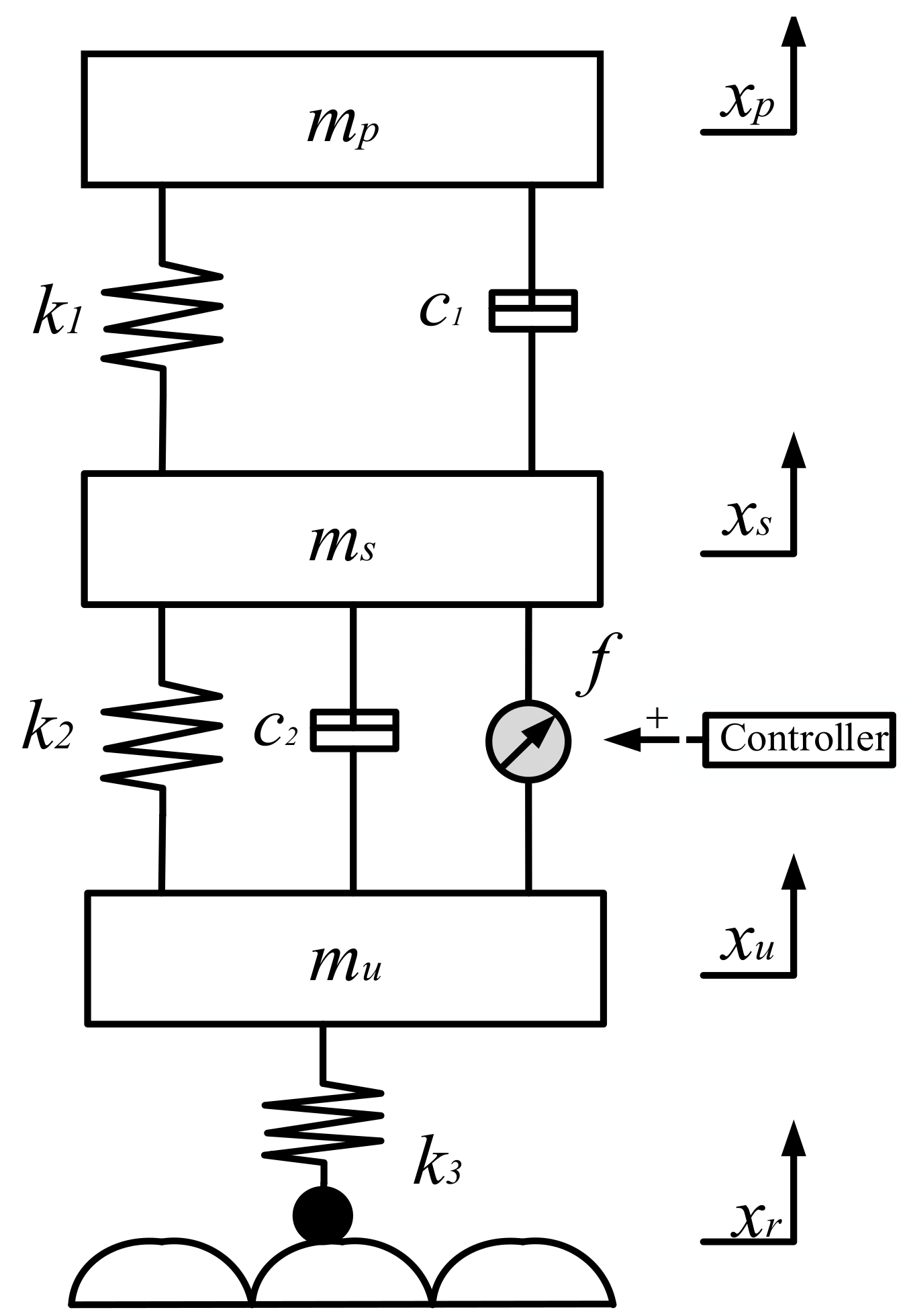
To understand the vibration characteristics of the vehicle under random road excitation, a vehicle model is established. The following assumptions are used to reduce a complex automobile model to a 3-DOF (mass) vibration system. Figure 1 presents a quarter-vehicle active suspension model with time-delay control. The vehicle model is simplified as a three-degree-of-freedom system. The components of the structure include passengers, car body mass, and wheel mass. Because of its simplicity, the quarter vehicle model is usually used to evaluate the performance of active and passive suspension systems.

Figure 1.
3-DOF seat model with time-delay control system.
2.1. Vehicle Model Assumptions
When the value of suspension mass distribution coefficient is close to 1, the vertical vibrations of the front and rear suspension mass are almost independent. The vehicle suspension system can be simplified to a 1/4 vehicle vibration system. The distances from the center of mass to the front and rear axes are a and b. The square of the turning radius of the body around the y-axis is .
- (1)
- Body, engine, frame, front, and rear axles are rigid. Body and frame are rigidly connected.
- (2)
- The car runs in a straight line at a constant speed v. The tire keeps in contact with the ground without jumping.
- (3)
- The automobile structure is symmetrical to the vertical plane. The road roughness of the left and right rut is the same. This means that the vehicle has no roll vibration, lateral displacement, or yaw motion. It only takes into account vertical vibrations.
- (4)
- Vehicle suspension stiffness tire stiffness and seat stiffness are linear functions of displacement. Suspension damping and seat damping are linear functions of relative velocity. Tire damping is ignored.
- (5)
- The contact mass of the car body is 0; i.e., the mass of the front and rear parts of the car body are independent of each other.
- (6)
- The person is located directly above the axle and is fixed.
The simplified vehicle model is shown in Figure 1 based on the above assumptions.
In Figure 1, is the mass of a human body; is the mass of the body part, including all car parts of the body spring suspension; is the unsprung mass, that is, the tire mass; k1 is the seat stiffness; k2 is the body suspension stiffness; k3 is tire stiffness; c1 is the seat damping; c2 is the body suspension damping; xp is the seat vertical displacement; xs is the body vertical displacement; xu is the wheel axle vertical displacement; xr is the excitation unevenness displacement.
2.2. Establishment of the Equation of Motion
The dynamic differential equation of the three-mass vehicle model can be obtained according to the D’Alembert principle.
The dynamic equations of the system include seat vertical motion equation, body mass vertical motion equation, and unsprung mass vertical motion equation:
Seat vertical motion equation:
Body mass vertical motion equation:
Vertical motion equation of unsprung mass:
where is the seat vertical beating acceleration; is the seat vertical beating speed; is the body mass vertical beating acceleration; is the body mass vertical beating speed; is the unsprung mass vertical beating acceleration; is the vertical beating speed of the unsprung mass; , where and represent the feedback gain and time-delay control amounts of the suspension active control force.
If the feedback gain of the suspension active control force and the time-delay control amount is 0, the active suspension system with time-delay control can be simplified to a traditional passive suspension system.
To transform Formulas (1)–(3), we can get:
The single-input multiple-output state-space method of the multiple-degree-of-freedom vibration system is used to analyze and modify the suspension system:
The state variable is ; the seat acceleration is ; the body acceleration is ; the suspension dynamic deflection is ; the tire dynamic deformation is ; the output is ; the input vector is ; the active control force of the suspension is . The state space equation of the active suspension control system with time-delay control shown in Equation (1) is:
where
3. Time-Delay Stability Analysis of Active Suspension with Time-Delay Control
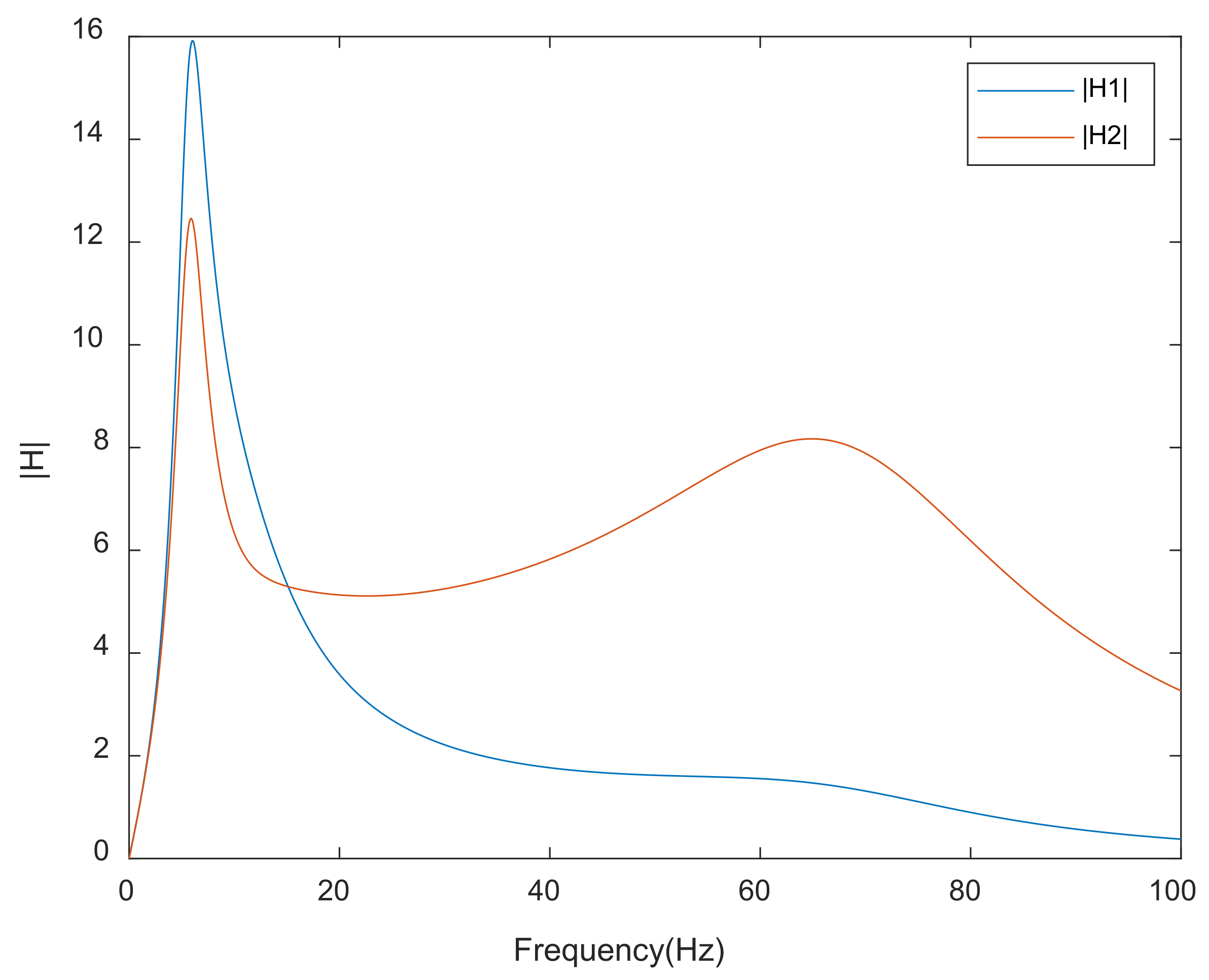
To analyze the peaks of occupant and body movement, the Fourier change is carried out according to Equation (4), the time domain characteristics are transformed into the frequency domain to study, and the frequency domain response function of occupant acceleration to road speed and the frequency domain response function of vehicle acceleration to road speed is obtained. The frequency response function curve is shown in Figure 2.
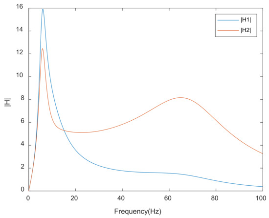
Figure 2.
Frequency response characteristic curve.
It can be seen in Figure 2 that frequency response characteristic curve |H1| of occupant acceleration. When there is no increase in control g = 0 and τ = 0, the maximum amplitude-frequency characteristic of the vehicle body is generally about 6 Hz, the maximum amplitude is 15.9, and then the amplitude decreases slowly with the increase in frequency. From the frequency response characteristic curve of body acceleration |H2|, it can be seen that when the control g = 0 and τ = 0 are not increased, the maximum amplitude-frequency characteristic of the body is generally within 5.9 Hz, and the maximum amplitude is 12.46. When it reaches 64.9 Hz, the body amplitude reaches the second peak value of 8.17 Hz. After that, the amplitude decreases slowly with increasing frequency.
System stability is a powerful guarantee for the safe and reliable operation of time-delay control. In this paper, the stability switching method is used to analyze the stability of time-delay feedback control [37,38,39].
To facilitate the analysis of system stability, the motion differential of the system, i.e., Equation (4), is normalized.
To make the analyzed physical quantities have a broader theoretical guiding significance, the following auxiliary variables are introduced:
For the convenience of writing, , can be marked as ,. Equations (1)–(3) can be simplified to:
According to the complete discriminant system of polynomials [40,41], it is assumed that is a polynomial of degree n.
is its discriminant sequence. Assume that the number of sign changes in the discriminant sequence symbol table is , where the number of non-zero terms is . If it satisfies , then the logarithm of the complex root of is ;
The number of distinct real roots of is . has multiple roots if and only if . The full-time-delay stability of the suspension system is solved by the full-time-delay stability judgment theorem of the time-delay dynamic system. The condition of full-delay stability for linear dynamical systems with a single delay is that the characteristic polynomial of the system is stable at . The coefficient of the first term of is 1, and its degree satisfies . In addition, at , the characteristic equation of the system has no real solution.
From Equations (6)–(8), the characteristic equation can be obtained as
The specific form is
where
For all , there is no real number solution if and only if the following polynomial is true:
See Appendix A for in the formula.
According to the Strum sequence discrimination method, the Strum sequence can be calculated by computing software.
In the formula, the number of polynomials is relatively high. The Maple program DISCR can be used to complete the program, as shown in Appendix A.
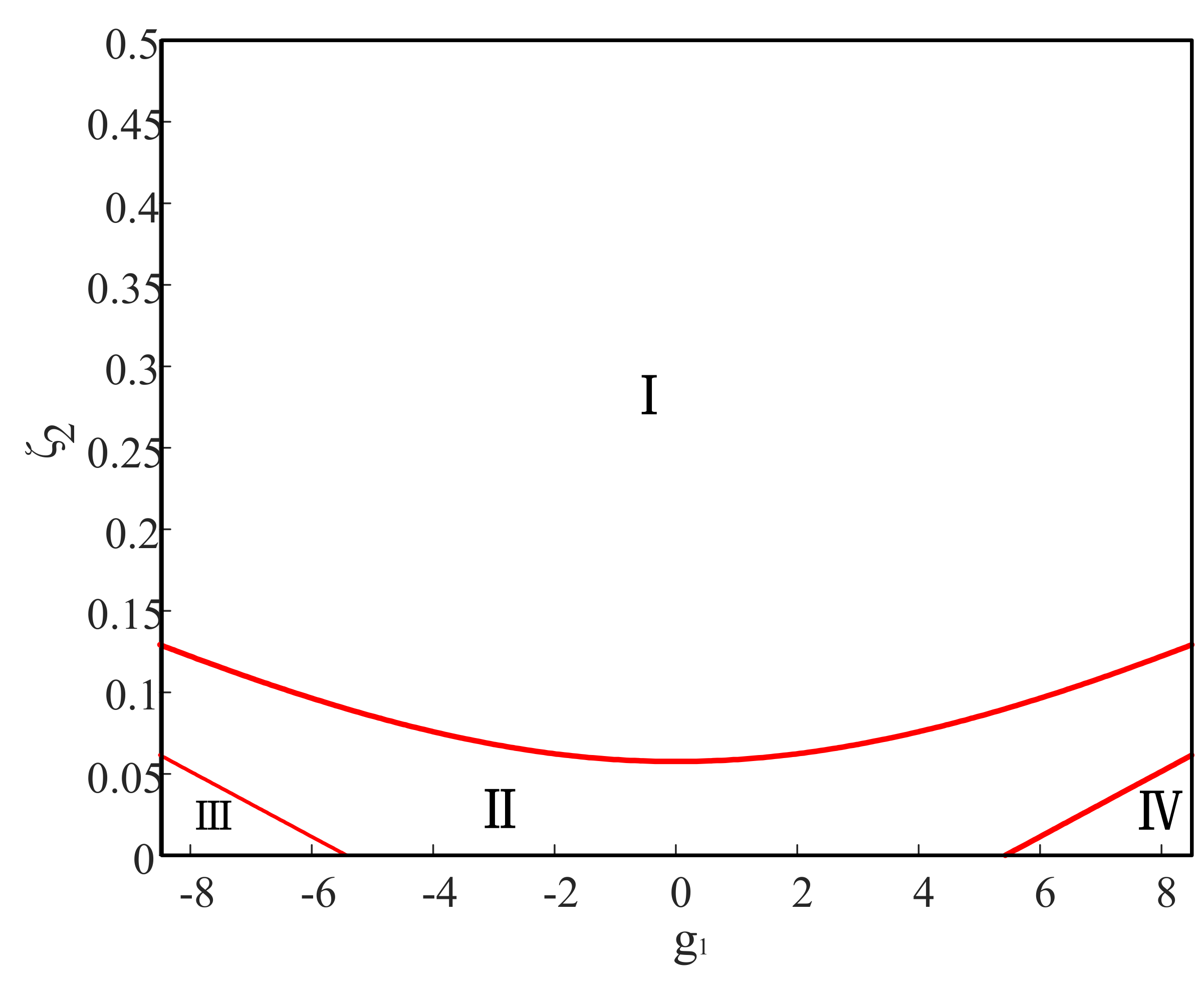
To realize polynomial without real roots, the sign change of the sequence of discriminant should satisfy according to the Strum test. Based on the parameters of a certain vehicle, as shown in Table 1, this paper studies the influence of suspension damping and control gain on the system’s time-delay stability. It takes as the adjustable damping to draw the values of and g within a certain value range that meet the conditions. The parameter plane satisfying the condition was divided into several regions according to the full delay stability condition, as shown in Figure 3. Different regions are different discriminant sequences, as shown in Table 2.

Table 1.
Vehicle suspension model parameters.
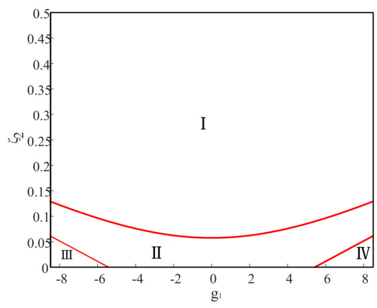
Figure 3.
The time-delay stability region of the active suspension in the parameter plane (, ).
Table 2.
The symbol sequence of the discriminant of active suspension and the number of real roots.
Theorem 1.
Assuming that the pure imaginary root of the characteristic equation of system (9) is not a solution of Q(iw) = 0, then [42]:
Ifhas no real root, then the system is fully time-delay stable; that is, the system does not undergo stability switching.
Ifhas only a positive single root w, then the corresponding delay-free system is asymptotically stable. There is somethat makes the system stable in. However, it is unstable for all; that is, the system has a stable switch. When the corresponding delay-free system is unstable, the system is unstable for all time delays; that is, the system does not undergo stability switching.
Ifhas more than one positive single root, the system will undergo a finite number of stability switches. It is ultimately unstable.
When the delay gradually increases from 0 to infinity, according to Table 2 and Theorem 1, it can be concluded as follows:
- (1)
- The regions I and PI are the full delay stability regions of the system. The corresponding system does not undergo stability switching.
- (2)
- The system switches between stable and unstable states as the parameter value increases in the region III at any time. After a finite number of stable alternation changes to the final instability, if all critical time-delays are arranged in order from small to large, as long as there are two adjacent values in the sequence that correspond to a large positive root of , the time-delay is increased. The system no longer has a stability switch and remains unstable from then on.
4. Suspension Time-Delay Control Parameter Optimization
4.1. The Establishment Method of Objective Function
This paper presents a new optimization method. When the complex excitation is known, the linear function is used to make the complex excitation equivalent in the discrete time interval. This means dividing continuous time into small periods of time. The linear function is equivalent to the complex excitation in each time interval. When the time interval is finely divided, the linear function can approximate the original complex excitation. In the continuous time interval, the amplitude of both is the same at each discrete time point. The optimization problem of complex excitation is transformed into the optimization problem of the normal force in the discrete time interval. This simplifies complex issues. At the same time, the external excitation is directly introduced into the solution process of time-delay control parameter optimization in the objective function. The quantitative relationship among the time-domain vibration response, time-delay control parameters, and external excitation are established.
Assume that is a complex excitation, and take the linear equivalent function . Among them, and are the equivalent parameters. In a small time interval of , then . Of these, is known. It is only necessary to solve for the equivalent parameters of and . Then, equivalent complex excitation is brought into Equations (1) to (3). It can solve the vibration response of the system at each time point tk by solving the dynamic equation of the system:
where , are the vibration displacement and velocity of the occupant at tk; , are the vibration displacement and velocity of the body mass at tk; and , are the vibration displacement and velocity of the unsprung mass at tk.
The vibration response of Equation (7) is brought into Equations (1)–(3) to obtain the vibration acceleration of the occupant, the body mass, and the unsprung vibration at time tk.
According to the vehicle’s ride comfort requirements, this paper takes the occupant vertical acceleration, body acceleration, suspension dynamic stroke, and tire dynamic load weighting as the optimization objective function and meets the ride comfort requirements to the greatest extent as the optimization objective. Due to the inconsistency of the units and magnitudes of each performance index, it will be divided by the corresponding passive suspension performance index value, and the fitness function obtained is as follows
where the weighting coefficients ,,, and are used as the weight coefficients of the evaluation function to measure the relative importance of each sub-objective function. In this paper, we take = 0.3, = 0.3, = 0.2, = 0.2 and , , , and to represent the corresponding performance of the passive suspension.
is the root mean square value of the occupant’s vertical acceleration:
is the root mean square value of body acceleration:
is the root mean square value of suspension dynamic deflection:
is the root mean square value of tire dynamic load:
where is the vibration acceleration of the occupant at time tk, is the vibration acceleration of the vehicle body at time tk, is the vertical displacement of vehicle vibration at time tk, and is the vertical displacement of wheel vibration at time tk.
Optimization Constraints
For the suspension dynamic deflection constraint, in order to prevent frequent collision with the buffer block when driving on bad roads, the dynamic stroke of the suspension must meet the inequality of Equation (16) within the safe stroke range:
where the maximum travel value of the suspension is represented by .
For tire grounding, in order to prevent the tire from falling off the ground during driving and cause driving safety problems, it is necessary to meet the inequality of Equation (17):
where the static load of the tire is represented by the calculation formula, which is as follows:
The formula of the mathematical model of the optimized objective function is as follows:
4.2. Time-Delay Control Parameter Optimization Based on Adaptive Weighted Particle Swarm Algorithm
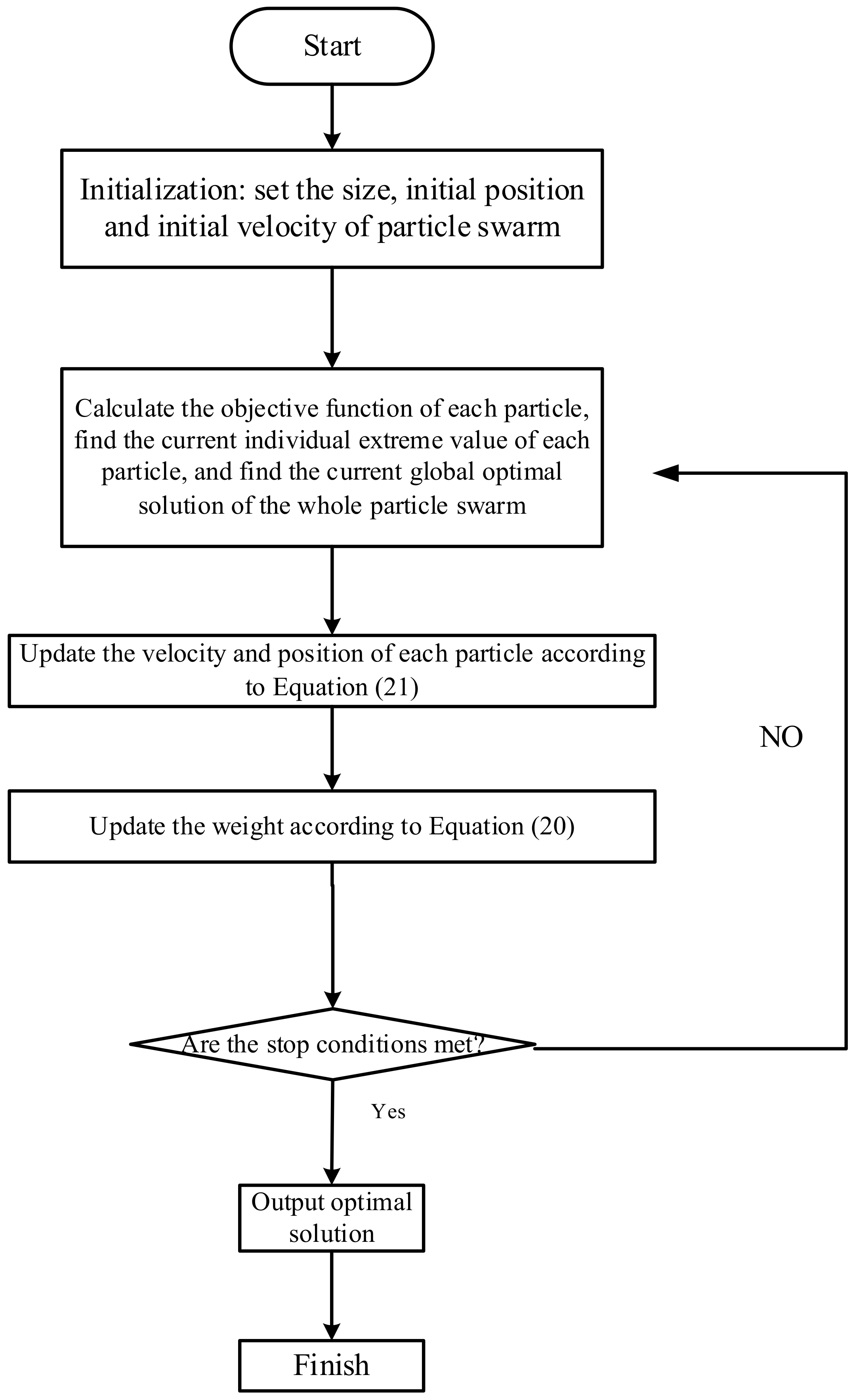
Particle Swarm Optimization (PSO) is an optimization algorithm based on the iterative operation. The system is initialized as a set of random solutions. It searches for the optimal value by iteration. An information sharing mechanism exists among particles. Pbest (individual extremum) or Gbest (global optimal solution) passes information to other particles. The particle search updates in the reciprocal flow follow the optimal solution and converge quickly. However, the PSO algorithm has the problem of “precocious” convergence and easily falls into the local best in the optimization process. To solve the problem of particle swarm, it combines the objective function characteristics established by Equation (19). In this paper, an adaptive inertia-weighted particle swarm optimization algorithm is used to optimize the delay feedback control parameters. The adaptive inertia weight particle swarm optimization (PSO) adjusts the inertia weight by using a nonlinear decreasing strategy. By balancing the global and local search capabilities of the particle swarm optimization algorithm, it can reduce the number of invalid iterations and reflect the advantages of fast convergence speed in the process of optimization [43,44,45].
4.2.1. Principle of the Optimization Algorithm
Because the large inertial factor is advantageous for jumping out of the local minimum point, it is convenient for global search. The smaller inertial factor is conducive to the accurate local search of the current search area, which uses algorithm convergence. Therefore, the PSO algorithm is prone to prematurity, and the oscillation phenomenon easily occurs near the global optimal solution in the late stage of the algorithm. The nonlinear dynamic inertia weight coefficient formula is used in this paper. The specific expression is as follows:
where and respectively represent the maximum and minimum values of W inertial weight coefficient, represents the current objective function value of particles, and and represent the average and minimum target values of all particles at present, respectively. In the above equation, the inertia weight changes automatically with the objective function value of the particle, so it is called the adaptive weight.
When the target value of each particle is generally consistent or locally optimal, it will increase the inertia weight. When the target value of each particle is relatively dispersed, it will reduce the inertia weight. At the same time, for particles whose target function value is better than the average target value, the factor of the corresponding inertial weight is small and protects the particle. For the particle whose target function value is different from the average target value, its corresponding inertial weight factor can make the particle closer to a better search area.
4.2.2. The Steps of Adaptive Weighted Particle Swarm Optimization
- 1.
- The position and velocity of each particle in the population are randomly initialized.
- 2.
- The fitness of each particle is evaluated. The current position and fitness value of each particle are stored in the Pbest of each particle. The location and fitness value of all the individuals are stord with the best fitness value in Pbest in Gbest.
- 3.
- The following formula is used to update the velocity and displacement of the particle:where is the update speed of the particle; is the updated displacement of the particle; r1 and r2 are random constants generated in [0,1]; and , are learning factors.
- 4.
- The weight is updated: .
- 5.
- For each particle, its fitness is compared to the best position it passes through. If the result is good, it takes it as the current best position. Comparing all current Pbest and Gbest values, Gbest is updated.
- 6.
- If the stop condition (generally the number of iterations or the preset accuracy of operation) is met, the search will stop and the results will be output. Otherwise, return to 3 to continue the search.
Flow chart of adaptive weight particle swarm optimization algorithm (as shown in Figure 4).

Figure 4.
Flow chart of adaptive weight particle swarm optimization algorithm.
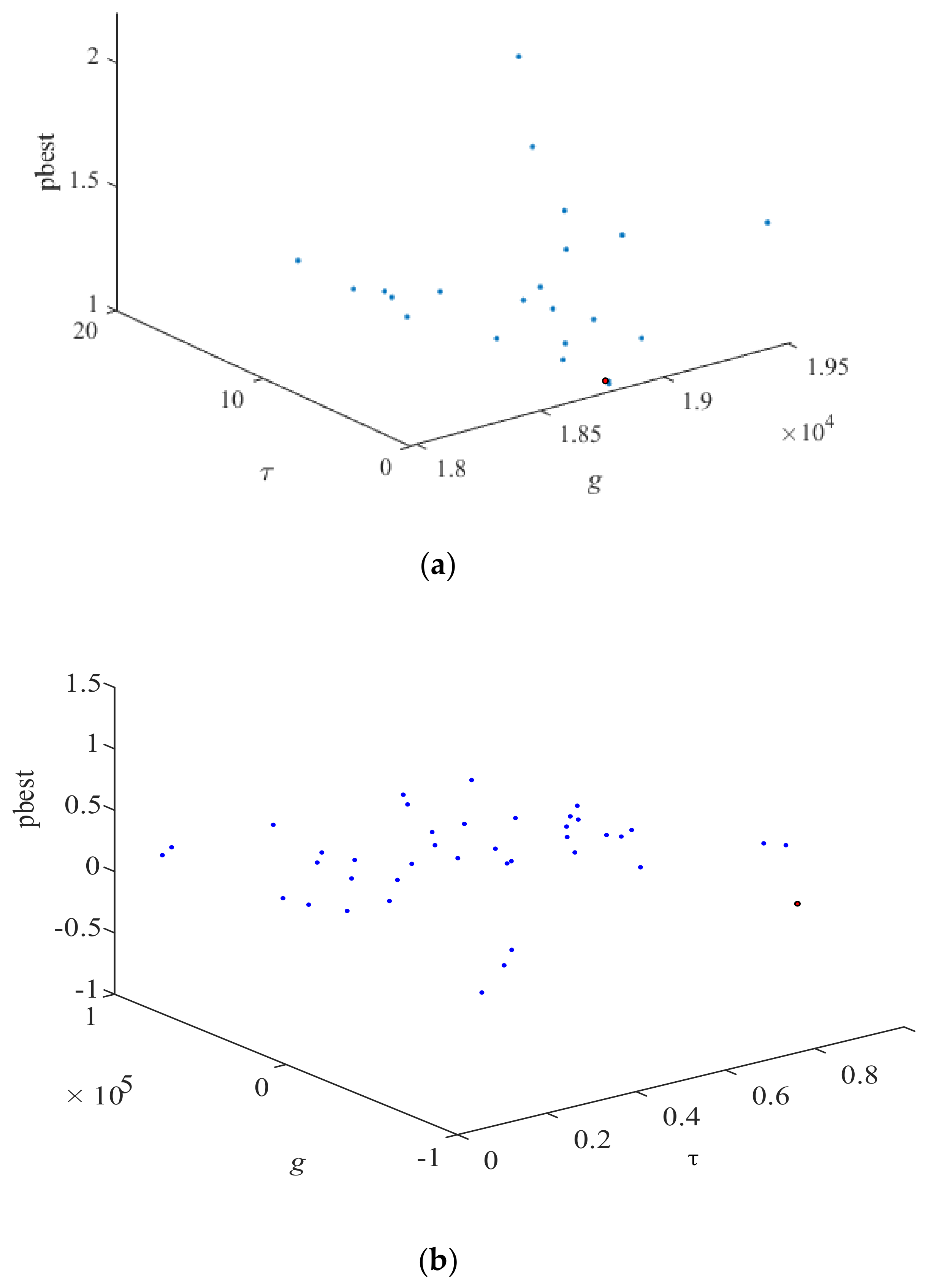
In the optimization process, the suspension parameters of a vehicle are referred to (as shown in Table 1 [46]). To more accurately search for the optimal individual extreme value and global optimal solution, 40 particles were randomly selected for iterative optimization. The maximum inertial weight of the learning factor is 0.9, and the minimum inertial weight is 0.6. After 100 iterations, the variation diagram of the iteration number of the fitness function of the suspension performance index is shown in Figure 5. It can be seen that with the continuous evolution of the population, the fitness function value of the optimal individual decreases rapidly. The number of invalid iterations is lower, and the convergence is fast. Finally, the global optimal control parameters under harmonic excitation and random excitation are obtained: g = 18,815.1534673518, τ = 0.868044394480619. g1 = −33,108.79988701554, τ2 = 0.992053286298810 It is carried to the I region of , , in which the feedback control parameters can be determined in the time-delay stability region. According to Theorem 1, the control system at this time is stable with full delay, and the system does not have stability switching; that is, the system is stable.
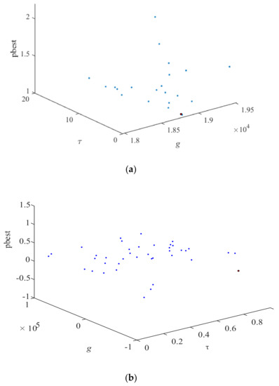
Figure 5.
Time-delay control parameter-change diagram. (a) Time-delay parameter-change diagram under harmonic excitation. (b) Time-delay parameter-change graph under random excitation.
5. Dynamic Performance Simulation and Analysis
5.1. Suspension Dynamic Performance Analysis under Harmonic Excitation Input
At present, the evaluation index of human comfort is the weighted root mean square value of acceleration proposed by ISO2631 standard.
The calculation formula of root mean square value of weighted acceleration is
where is the root mean square value of longitudinal acceleration, is the root mean square value of lateral acceleration, and is the root mean square value of vertical acceleration.
Because this paper mainly evaluates the impact of vertical vibration on comfort, only the root mean square value of vertical vibration weighted acceleration is calculated. The formula for calculating the frequency weighted value of the root mean square value of vibration-frequency-weighted acceleration at different frequencies is
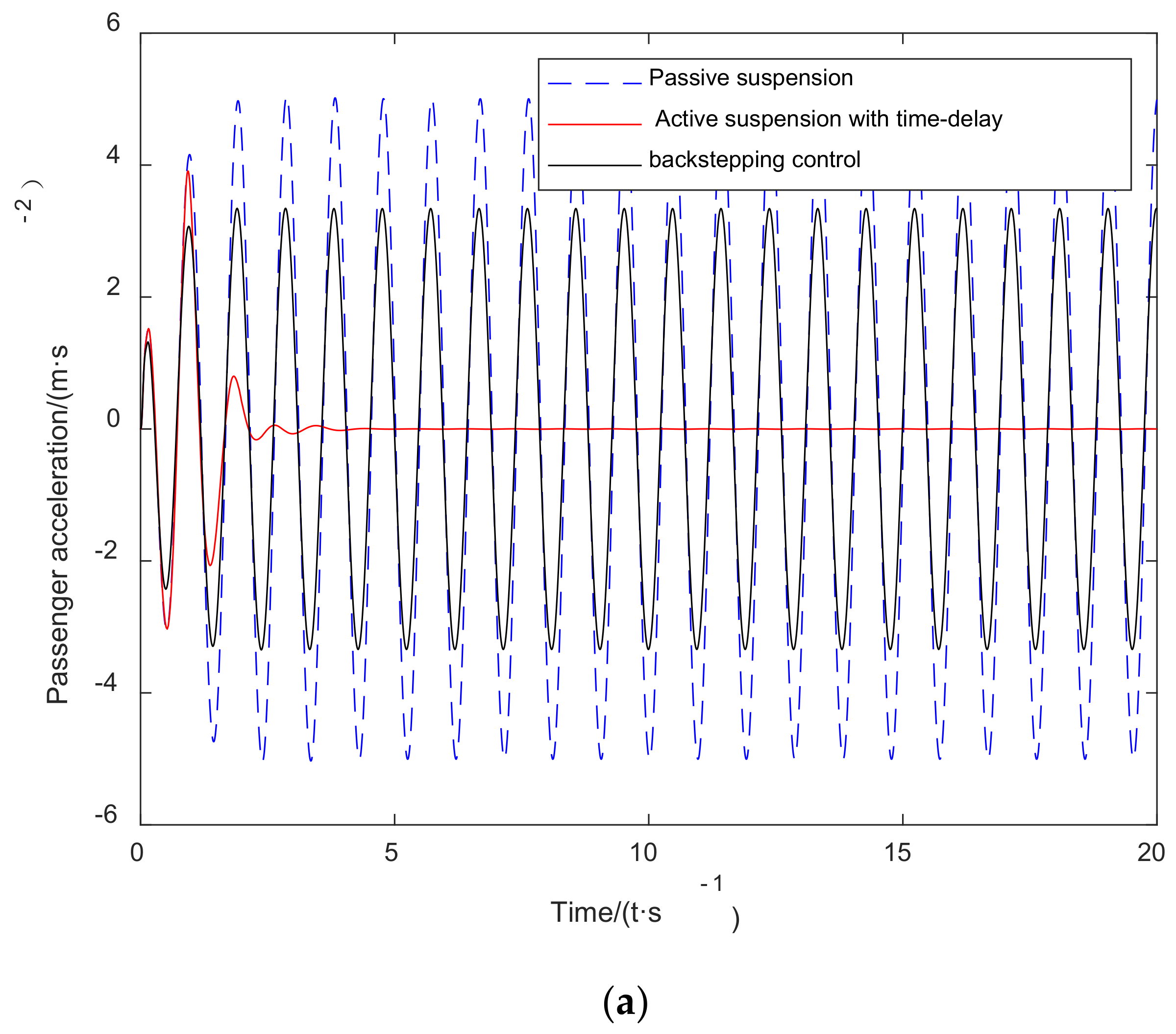
To verify the feasibility and effectiveness of the optimized time-delay control parameter method and the time-delay feedback-vibration-reduction control method proposed in this paper, the passive suspension, the active suspension based on backstepping control, and the time-delay active suspension with optimal parameter feedback control are combined. The performance indicators of the rack are compared by time-domain simulation, and the results of the simulation comparison are shown in Figure 6 [47]. To quantitatively analyze the damping performance of the active suspension with time-delay control, Table 3 lists the passengers of the time-delay active suspension system, passive suspension system, and back-control active suspension system under the optimal parameters. Root mean square value of acceleration, body acceleration, and suspension dynamic deflection, tire dynamic load, are used to calculate the corresponding change in percentage.
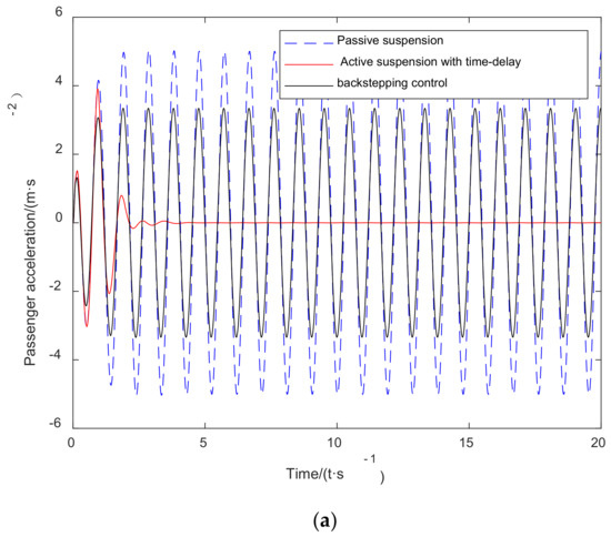
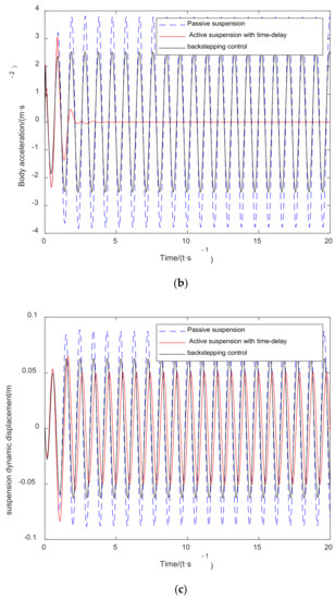
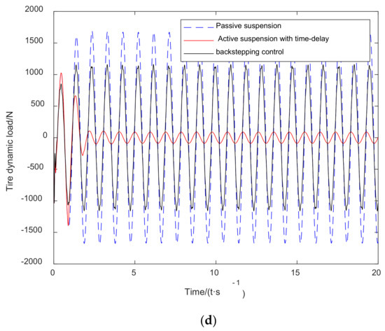
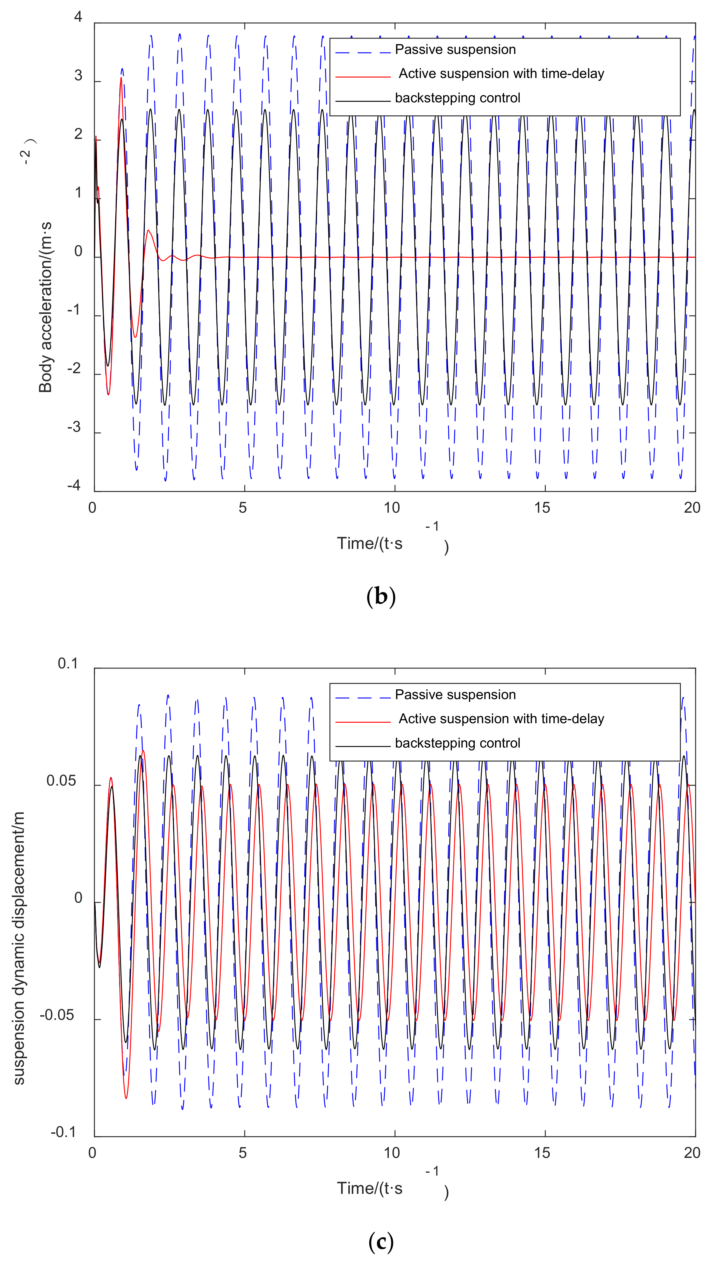
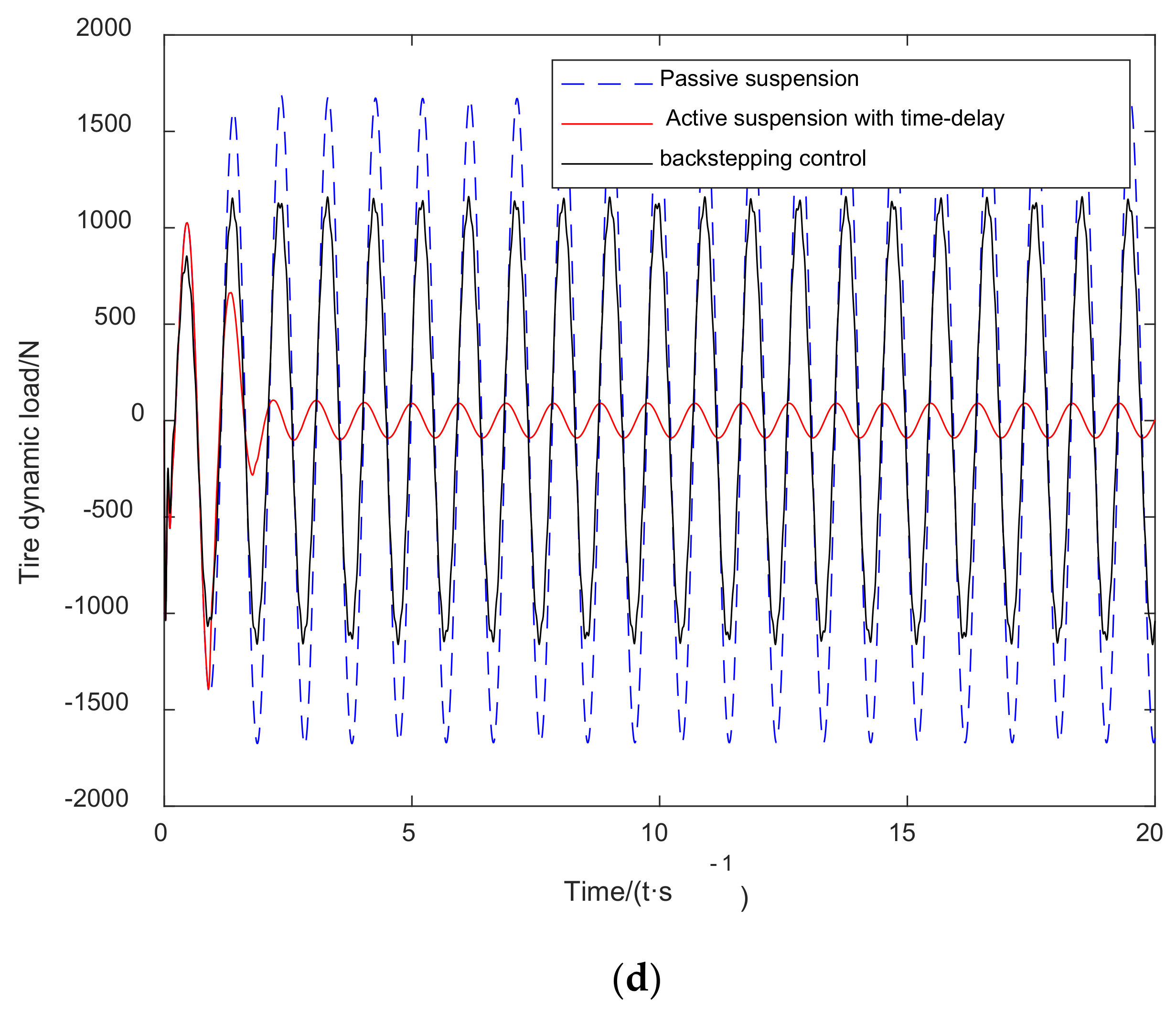
Figure 6.
Comparison chart of suspension performance simulation results under harmonic excitation; (a) Passenger vertical acceleration comparison chart; (b) vehicle body vertical acceleration comparison chart; (c) suspension dynamic deflection comparison chart; (d) tire dynamic load comparison chart.
Table 3.
Suspension performance root mean square value comparison table.
As can be seen from Figure 6, the performance of the active suspension system with time-delay control under harmonic excitation is significantly improved compared with that of the passive suspension system. For the passive suspension system, the fluctuation range of passenger vertical acceleration is 3.815 m/s2 ~ −3.815 m/s2, and the fluctuation range of body vertical acceleration is 5.046 m/s2 ~ −5.046 m/s2. The fluctuation range of the suspension dynamic displacement is 0.08752 m ~ −0.08752 m, and the fluctuation range of the tire dynamic load is 1671 N ~ −1671 N. Meanwhile, for the active suspension system based on backstepping control, the fluctuation range of passenger vertical acceleration is 3.344 m/s2 ~ −3.344 m/s2, the fluctuation range of body vertical acceleration is 2.522 m/s2 ~ −2.522 m/s2, and the fluctuation range of suspension dynamic displacement is 0.0628 m ~ −0.0628 m. The range of the tire dynamic load fluctuation is 1157 N ~ −1157 N. However, the time-delay control strategy adopted in this paper determines the passenger vertical acceleration, and the vibration of the car body is completely eliminated after the vertical acceleration is stabilized. The suspension-dynamic-displacement fluctuation range is 0.05043 m ~ −0.05043 m, tire dynamic load fluctuation range is 89.77 N ~ −89.77 N. Compared with the ordinary active-suspension backstepping-control strategy, the time-delay damping control active suspension designed in this paper significantly reduces the fluctuation range of the suspension performance index.
By comparing the values in Table 3, it can be seen that the active suspension control strategy with time-delay control designed in this paper can optimize the passenger vertical acceleration by 90.42%, the body vertical acceleration by 84.08%, the suspension dynamic deflection by 32.62%, and the tire dynamic load by 85.57% compared with the passive suspension performance. Compared with the active suspension based on inverse control, the active suspension control strategy with time-delay control designed in this paper can optimize the passenger vertical acceleration by 82.71%, the body vertical acceleration by 83.13%, the suspension dynamic deflection by 13.50%, and the tire dynamic load by 80.29%. Active suspension with time-delay control improves the performance of suspension significantly. This shows that the method proposed in this paper achieves the purpose of improving suspension comfort.
5.2. External Incentive Input
To further evaluate the feasibility and effectiveness of the method of optimizing the time-delay control parameters proposed in this paper, random excitation is selected as the vertical disturbance to the wheel axle, and the 3-DOF suspension established model is subjected to random excitation as an example for time-domain analysis. In this paper, a time-domain model of random excitation is established by the superposition of random sine waves. The power spectrum density of road displacement is expressed by . In time frequency , it is divided into n small intervals. The power spectrum density value corresponding to the central frequency of each cell is taken to replace the value of the whole cell. Then, a sine wave function with an intermediate frequency (i = 1, 2, ⋯, n) and standard deviation is found. Such a sine wave function can be expressed as [48]:
Equation (24) is superimposed on the sine wave function corresponding to each cell, and the time domain expression of the random displacement input is obtained as follows:
where random numbers are uniformly distributed on . is the time domain expression of random excitation displacement.
5.3. Simulation Results
After obtaining the time-delay control parameters under random excitation through the adaptive particle swarm optimization algorithm, according to the differential equation of motion of the vehicle’s active suspension system and external excitation input, the passive suspension, the active suspension based on backstepping control, and the external excitation input are established. A simulation model of active suspension with time-delay control and a comparative analysis of its dynamic performance are provided. Under the condition of random excitation, the changed results of root mean square values of passenger acceleration, body acceleration, suspension dynamic deflection, and tire dynamic load are shown in Table 4.
Table 4.
Suspension performance root mean square value comparison table.
By comparing the values in Table 4, it can be seen that vehicle comfort is measured by vehicle body acceleration and passenger acceleration. The two kinds of active suspension are improved to some extent compared to the passive suspension. Two kinds of active control suspension are affected by random excitation. The active suspension eliminates the external force and causes the suspension dynamic to travel a larger distance than the passive suspension dynamic travels. However, it is within the scope of the design [49]. Compared with the passive suspension system and the active suspension based on inverse control, the performance of the active suspension system with time-delay control under random excitation has been significantly improved. For the passive suspension system, the fluctuation range of passenger vertical acceleration is 0.4647 m/s2 ~ −0. 4585 m/s2, and the fluctuation range of body vertical acceleration is 0.6239 m/s2 ~ −0.6207 m/s2. The fluctuation range of suspension dynamic displacement is 0.00728 m ~ −0.00788 m, and the fluctuation range of tire dynamic load is 238.3 N ~ −238.6 N. For the active suspension system based on backstepping control, the fluctuation range of passenger vertical acceleration is 0.4478 m/s2 ~ −0.4457 m/s2, and the fluctuation range of body vertical acceleration is 0.0330 m/s2 ~ −0.3309 m/s2. The fluctuation range of suspension dynamic displacement is 0.01522 m ~ −0.11418 m, and the fluctuation range of tire dynamic load is 155.1 N ~ −154.8 N. However, the time-delay control damping control strategy adopted in this paper makes the fluctuation range of passenger vertical acceleration 0.2876 m/s2 ~ −0.2768 m/s2, and the fluctuation range of vehicle body vertical acceleration 0.2941 m/s2 ~ −0.3144 m/s2. Suspension dynamic displacement fluctuation range is 0.00742 m ~ −0.007869 m, and tire dynamic load fluctuation range is 140.1 N ~ −135.5 N. Compared with the performance of the passive suspension, the active suspension control strategy with time-delay control designed in this paper can optimize passengers’ vertical acceleration by 29.99%. The body vertical acceleration was optimized by 47.23%, and the tire dynamic load was optimized by 40.26%. Compared with the active suspension based on inverse control, the active suspension control strategy with delay feedback control is designed in this paper. It can optimize passenger vertical acceleration by 13.63%, body vertical acceleration by 28.38%, and tire dynamic load by 1.42%. Through quantitative analysis, it can be concluded that the active suspension with time-delay control has better system dynamic performance and higher control precision than the active suspension with inverse control, which has an obvious effect on the improvement of suspension vibration damping performance.
7. Conclusions
In this paper, the 3-DOF quarter vehicle active suspension is employed as the control object, and the vehicle ride comfort is optimized as the target. A linear function equivalent excitation method is proposed to establish the objective function, and the optimal parameter time-delay control active suspension is designed. The adaptive weighted particle-swarm optimization algorithm is used to obtain the optimal delay feedback control parameters. The feedback control parameters are obtained by stability analysis and time-domain simulation as follows:
- 1.
- In this paper, the stability switching method is used for the first time to analyze the stability interval of 3-DOF time-delay controlled active suspension, which deduces the system stability conditions related to the Strum sequence and the feedback control parameters. The results show that the time-delay control parameters can change the stability of the system.
- 2.
- A linear excitation function is equivalent to excitation cup design. It can estimate the disturbance in real time to improve the control accuracy.
- 3.
- Through simulation analysis, the time-delay control algorithm designed in this paper is used to compare the inverse control and the passive suspension control. In the time domain of different working conditions, especially in harmonic excitation, the damping performance of vehicle acceleration and passenger acceleration is obviously improved. This can provide a useful reference for further experimental investigation.
Author Contributions
Writing—original draft, K.W.; software K.W., Y.C.; Writing—review and editing, K.W. and C.R. All authors have read and agreed to the published version of the manuscript.
Funding
This work is supported by National Natural Science Foundation of China (Grant No. 51275280).
Institutional Review Board Statement
Not applicable.
Informed Consent Statement
Not applicable.
Data Availability Statement
Not applicable.
Conflicts of Interest
The authors declare no conflict of interest.
Appendix A
The discr program is as follows
- discr: = proc(poly,var)
- local f,g,tt,d,bz,i,ar,j,mm,dd:
- f: = expand(poly): d: = degree(f,var):
- g: = tt*var^d + diff(f,var):
- with(linalg):
- bz: = subs(tt = 0,bezout(f,g,var)):ar: = []:
- for i to d do
- ar: = [op(ar),row(bz,d + 1-i..d + 1-i)] od:
- mm: = matrix(ar):dd: = []:
- for j to d do
- dd: = [op(dd),det(submatrix(mm,1..j,1..j))] od:
- dd: = map(primpart,dd)
- end:
For example, for polynomial:
Using discr, the discriminant sequence can be calculated as [1, 1, 1, 1, −1, 1, 1, −1, 1, 1, −1, 1].
References
- Qi, H.; Chen, Y.; Zhang, N.; Zhang, B.; Wang, D.; Tan, B. Improvement of both handling stability and ride comfort of a vehicle via coupled hydraulically interconnected suspension and electronic controlled air spring. Proc. Inst. Mech. Eng. Part D J. Automob. Eng. 2020, 234, 552–571. [Google Scholar] [CrossRef]
- Qi, H.; Zhang, N.; Chen, Y.; Tan, B. A comprehensive tune of coupled roll and lateral dynamics and parameter sensitivity study for a vehicle fitted with hydraulically interconnected suspension system. Proc. Inst. Mech. Eng. Part D J. Automob. Eng. 2021, 235, 143–161. [Google Scholar] [CrossRef]
- Wang, M.; Zhang, B.; Chen, Y.; Zhang, N.; Zhang, J.; Chen, S. Frequency-Based Modeling of a Vehicle Fitted With Roll-Plane Hydraulically Interconnected Suspension for Ride Comfort and Experimental Validation 2020. IEEE Access 2021, 8, 1091–1104. [Google Scholar] [CrossRef]
- Qi, H.; Zhang, B.; Zhang, N.; Zheng, M.; Chen, Y. Enhanced lateral and roll stability study for a two-axle bus via hydraulically interconnected suspension tuning. SAE Int. J. Veh. Dyn. Stab. NVH 2019, 3, 5–18. [Google Scholar] [CrossRef]
- Tan, B.; Wu, Y.; Zhang, N.; Zhang, B.; Chen, Y. Improvement of ride quality for patient lying in ambulance with a new hydro-pneumatic suspension. Adv. Mech. Eng. 2019, 11, 1687814019837804. [Google Scholar] [CrossRef] [Green Version]
- Zeng, M.; Tan, B.; Ding, F.; Zhang, B.; Zhou, H.; Chen, Y. An experimental investigation of resonance sources and vibration transmission for a pure electric bus. Proc. Inst. Mech. Eng. Part D J. Automob. Eng. 2020, 234, 950–962. [Google Scholar] [CrossRef]
- Tan, B.; Chen, Y.; Liao, Q.; Zhang, B.; Zhang, N.; Xie, Q. A condensed dynamic model of a heavy-duty truck for optimization of the powertrain mounting system considering the chassis frame flexibility. Proc. Inst. Mech. Eng. Part D J. Automob. Eng. 2020, 234, 2602–2617. [Google Scholar] [CrossRef]
- Zheng, M.; Peng, P.; Zhang, B.; Zhang, N.; Wang, L.; Chen, Y. A new physical parameter identification method for two-axis on-road vehicles: Simulation and experiment. Shock Vib. 2015, 2015, 1–9. [Google Scholar] [CrossRef] [Green Version]
- Jiregna, I.; Sirata, G. A review of the vehicle suspension system. J. Mech. Energy Eng. 2020, 4, 109–114. [Google Scholar] [CrossRef]
- Xu, J. Advances of research on vibration control. Chin. Q. Mech. 2015, 36, 547–565. [Google Scholar]
- Zhang, J.; Zhang, B.; Zhang, N.; Wang, C.; Chen, Y. A novel robust event-triggered fault tolerant automatic steering control approach of autonomous land vehicles under in-vehicle network delay. Int. J. Robust Nonlinear Control 2021, 31, 2436–2464. [Google Scholar] [CrossRef]
- Hu, H.; Wang, Z.H. Advances in Dynamics of Controlled Mechanical Systems with Time-Delay. Prog. Nat. Sci. 2000, 7, 801–811. [Google Scholar]
- Filipovic, D.; Olgac, N. Delayed resonator with speed feedback–design and performance analysis. Mechatronics 2002, 12, 393–413. [Google Scholar] [CrossRef]
- Olgac, N.; Holm-Hansen, B.T. A novel active vibration absorption technique: Delayed resonator. J. Sound Vib. 1994, 176, 93–104. [Google Scholar] [CrossRef]
- Olgac, N.; Holm-Hansen, B.T. Design considerations for delayed-resonator vibration absorbers. J. Eng. Mech. 1995, 121, 80–89. [Google Scholar] [CrossRef]
- Olgac, N.; Hosek, M. Active vibration absorption using delayed resonator with relative position measurement. J. Vib. Acoust. 1997, 119, 131–136. [Google Scholar] [CrossRef]
- Chen, Y.; Mendoza, A.S.E.; Griffith, D.T. Experimental and numerial study of high-order complex curvature mode shape and mode coupling on a three-bladed wind turbine assembly. Mech. Syst. Signal Process. 2021, 160, 107873. [Google Scholar] [CrossRef]
- Chen, Y.; Avitabile, P.; Page, C.; Dodson, J. A polynomial based dynamic expansion and data consistency assessment and modification for cylindrical shell structures. Mech. Syst. Signal Process. 2021, 154, 107574. [Google Scholar] [CrossRef]
- Chen, Y.; Joffre, D.; Avitabile, P. Underwater dynamic response at limited points expanded to full-field strain response. J. Vib. Acoust. 2018, 140, 051016. [Google Scholar] [CrossRef] [Green Version]
- Saeed, N.A.; El-Ganaini, W.A. Time-delayed control to suppress the nonlinear vibrations of a horizontally suspended Jeffcott-rotor system. Appl. Math. Model. 2017, 44, 523–539. [Google Scholar] [CrossRef]
- Eissa, M.; Kamel, M.; Saeed, N.; El-Ganaini, W.A.; El-Gohary, H.A. Time-delayed positive-position and velocity feedback controller to suppress the lateral vibrations in nonlinear Jeffcott-rotor system. Menoufia J. Electron. Eng. Res 2018, 27, 261–278. [Google Scholar] [CrossRef]
- Saeed, N.; El-Ganini, W.A.; Eissa, M. Nonlinear time delay saturation-based controller for suppression of nonlinear beam vibrations. Appl. Math. Model. 2013, 37, 8846–8864. [Google Scholar] [CrossRef]
- Maccari, A. Vibration control for the primary resonance of a cantilever beam by a time delay state feedback. J. Sound Vib. 2003, 259, 241–251. [Google Scholar] [CrossRef]
- Udwadia, F.E.; von Bremen, H.F.; Kumar, R.; Hosseini, M. Time delayed control of structural systems. Earthq. Eng. Struct. Dyn. 2003, 32, 495–535. [Google Scholar] [CrossRef]
- Zhao, Y.Y.; Xu, J. Using time-delay feedback to control the vibration of a self-parametric vibration system. Chin. J. Theor. Appl. Mech. 2011, 43, 894. [Google Scholar]
- Zhao, Y.Y.; Xu, J. Time-delay dynamic vibration absorber and its influence on main system vibration. Adv. Mech. 2006, 12, 13. [Google Scholar]
- Zhao, Y.Y.; Xu, J. Vibration reduction mechanism of time-delay nonlinear dynamic vibration absorber. Chin. J. Theor. Appl. Mech. 2008, 40, 98–106. [Google Scholar]
- Zhao, Y.Y.; Xu, J. The role of time-delay feedback control in self-parametric dynamic vibration absorber. Acta Mech. Solida Sin. 2007, 28, 347–354. [Google Scholar]
- Chen, L.X.; Cai, G.P. Experimental study on active control of a rotating flexible beam with time delay. Chin. J. Theor. Appl. Mech. 2008, 40, 520–527. [Google Scholar]
- Chen, L.X.; Cai, G.P. Experimental study on time-delay variable structure control of a flexible beam subjected to forced vibration. Chin. J. Theor. Appl. Mech. 2009, 41, 410–417. [Google Scholar]
- Zhao, T.; Chen, L.X.; Cai, G. Theoretical and experimental research on time-delay H∞ control of flexible boards. Chin. J. Theor. Appl. Mech. 2011, 43, 1043–1053. [Google Scholar]
- Chen, L.X.; Cai, G.P. Design Method of Multiple Time Delay Control Law for Active Structural Vibration Control. Appl. Math. Mech. 2009, 30, 1318–1326. [Google Scholar] [CrossRef]
- Phu, D.X.; Shin, D.K.; Choi, S.B. Design of a new adaptive fuzzy controller and its application to vibration control of a vehicle seat installed with an MR damper. Smart Mater. Struct. 2015, 24, 085012. [Google Scholar] [CrossRef]
- Phu, D.X.; Quoc Hung, N.; Choi, S.B. A novel adaptive controller featuring inversely fuzzified values with application to vibration control of magneto-rheological seat suspension system. J. Vib. Control 2018, 24, 5000–5018. [Google Scholar] [CrossRef]
- Phu, D.X.; Mien, V.; Choi, S.-B. A New Switching Adaptive Fuzzy Controller with an Application to Vibration Control of a Vehicle Seat Suspension Subjected to Disturbances. Appl. Sci. 2021, 11, 2244. [Google Scholar] [CrossRef]
- Phu, D.X.; Mien, V. Robust control for vibration control systems with dead-zone band and time delay under severe disturbance using adaptive fuzzy neural network. J. Frankl. Inst. 2020, 357, 12281–12307. [Google Scholar] [CrossRef]
- Wang, Z.H.; Hu, H.Y. Stability switches of time-delayed dynamic systems with unknown parameters. J. Sound Vib. 2000, 233, 215–233. [Google Scholar] [CrossRef]
- Wang, Z.H.; Hu, H.Y. Stability of force control system with sampling feedback. Chin. J. Theor. Appl. Mech. 2016, 48, 1372–1381. [Google Scholar]
- Fu, W.Q.; Pang, H.; Kai, L.; Qiang, L. Modeling and Stability Analysis of Semi-active Suspension with Time-delay Ceiling Damping. Mech. Sci. Technol. Aerosp. Eng. 2017, 36, 213–218. [Google Scholar]
- Yang, L.; Hou, X.R.; Zeng, Z. Complete discriminant system of polynomials. Sci. China Ser. E Technol.Sci. 1996, 26, 424–441. [Google Scholar]
- Yang, L.; Zhang, J.Z.; Xiaorong, H. Nonlinear Algebraic Equation System and Automated Theorem Proving; Shanghai Scientific and Technological Education Publishing House: Shanghai, China, 2001; pp. 137–179. [Google Scholar]
- Wang, Z.H. Stability of High Dimensional Time-Delay Dynamical Systems; Nanjing University of Aeronautics and Astronautics: Nanjing, China, 2000; pp. 18–25. [Google Scholar]
- Liu, W.; Wang, Z.; Yuan, Y.; Zeng, N.; Hone, K.; Liu, X. A novel sigmoid-function-based adaptive weighted particle swarm optimizer. IEEE Trans. Cybern. 2021, 51, 1085–1093. [Google Scholar] [CrossRef]
- Kennedy, J.; Eberhart, R. Particle swarm optimization. In Proceedings of the ICNN’95-International Conference on Neural Networks, Perth, WA, Australia, 27 November–1 December 1995; Volume 4, pp. 1942–1948. [Google Scholar]
- Huan, R.H.; Chen, L.X.; Sun, J.Q. Multi-objective optimal design of active vibration absorber with delayed feedback. J. Sound Vib. 2015, 339, 56–64. [Google Scholar] [CrossRef]
- Yu, Y.; Lei-Lei, D.; Zhang-Cheng, Z.; Song, Y.; Jian, Y.N. Design and analysis of vehicle seat suboptimal control active suspension. J. Beijing Univ. Posts Telecommun. 2021, 44, 87–93. [Google Scholar]
- Li, J.; Xu, D.M. Adaptive Backstepping Sliding Mode Control for Non-matching Uncertain Nonlinear Systems. Control Decis. 1999, 65, 47–51. [Google Scholar]
- Zhang, Y.L. Reconstruction of the time-domain model of random road irregularity elevation with harmonic superposition method. Trans. Chin. Soc. Agric. Eng. 2003, 19, 32–35. [Google Scholar]
- Crolla, D.; Yu, F. Vehicle dynamics and control; China People Communication Press: Beijing, China, 2004; Volume 309, pp. 23–43. [Google Scholar]
Publisher’s Note: MDPI stays neutral with regard to jurisdictional claims in published maps and institutional affiliations. |
© 2021 by the authors. Licensee MDPI, Basel, Switzerland. This article is an open access article distributed under the terms and conditions of the Creative Commons Attribution (CC BY) license (https://creativecommons.org/licenses/by/4.0/).