A Block Arnoldi Algorithm Based Reduced-Order Model Applied to Large-Scale Algebraic Equations of a 3-D Field Problem

Featured Application

This work has developed an adaptive multipoint model reduction model based on the Arnoldi algorithm to obtain reduced-order models of a 3-D temperature field.

Abstract

In simulations of three-dimensional transient physics filled through a numerical approach, the order of the equation set of high-fidelity models is extremely high. To eliminate the large dimension of equations, a model order reduction (MOR) technique is introduced. In the existing MOR methods, the block Arnoldi algorithm-based MOR method is numerically stable, achieving a passively reduced order model. Nevertheless, this method performs poorly when it is applied to very wide-frequency transients. To eliminate this deficiency, multipoint MOR methods are emerging. However, it is hard to directly apply an existing multipoint MOR method to a 3-D transient field equation set. The implementation issues in a reduction process (such as the selection of expansion points, the number of moments matched at a point and the error bound) have not been explored in detail. In this respect, an adaptive multipoint model reduction model based on the Arnoldi algorithm is proposed to obtain the reduced-order models of a 3-D temperature field. The originality of this study is the proposal of a novel adaptive algorithm for selecting expansion points, matching moments automatically, using a posterior-error estimator based on temperature response coupled with a network topological method (NTM). The computational efficiency and accuracy of the proposed method are evaluated by the numerical results from solving the temperature field of a prototype insulated-gate bipolar transistor (IGBT).

1. Introduction

In computations of three-dimensional transient fields of a high-fidelity model, the order of the equation set is extremely high. It is thus infeasible to directly use the high-fidelity model to simulate the transient behavior of an electromagnetic device over a long-time span. To compromise the computational time and model accuracy performances, a model order reduction (MOR) technique is used to generate a reduced-order model to substitute the original high-fidelity one. The reduced-order model diminishes the computational complexity, utilizing less computational resources compared to the original system.

Different MOR techniques have been proposed and applied to combat the complexity of interconnected problems [1,2,3] and finite-element equations of electromagnetic problems [4,5,6,7]. However, there are few works oriented for 3-D temperature fields. Moreover, in addition to the solution efficiency, an MOR approach should also be compromised of different implementation criteria. Implementation issues include the number and generating mechanism of the expansion points, the approximate order of the model for each expansion point, and so on. In this direction, some MOR techniques have already been reported. For example, the Asymptotic Waveform Evaluation (AWE), as reported in [8], has focused on solving the number and generating mechanism of the expansion points by considering complex frequency hopping (CFH). Authors in [9,10,11] have focused on the error bound and selection of expansion points for Páde-via-Lanczos (PVL). In addition, authors in [12] have focused on the error bound and selection of expansion points for Efficient Nodal Order Reduction (ENOR) by embedding proper orthogonal decomposition (POD).

However, both AWE and ENOR use a recursive expression to explicitly compute the moments of the high-fidelity model. Therefore, AWE and ENOR are not numerically stable [13]. Although PVL is a powerful and efficient algorithm, it cannot preserve some physically feasible conditions such as model passivity [13]. On the other hand, in the MOR methods based on moment matching, the Passive Reduced-order Interconnect Macromodeling Algorithms (PRIMA), based on the Arnoldi method, are numerically stable and can preserve the passivity of the high-fidelity model in RLC circuits. Nevertheless, this method is difficult to directly employ on a high-fidelity model of a three-dimensional transient field since this methodology is intended to deal with interconnect circuit equations, which are different in form from 3-D transient field equations. Furthermore, the difficulty of applications in broadband situations for PRIMA has not been explored in detail in the literature. In this regard, we propose an adaptive multipoint model reduction model based on the Arnoldi algorithm to obtain the reduced-order models of a 3-D temperature field.

2. Proposed Order Reduction Methodology

2.1. Three-Dimensional Transient Temperature Field Problems

In general, the general equation set of a transient temperature filed can be formulated as [12]:

$$\mathit{B}\frac{d\mathit{T}}{dt}+\mathit{A}\mathit{T}(t)=\mathit{P}\mathit{J}(t)$$

(1)

where, $B\in {\Re }^{n\times n}$, $T\in {\Re }^{n\times 1}$, $A\in {\Re }^{n\times n}$, $P\in {\Re }^{n\times N}$, $J\in {\Re }^{N\times 1}$, ${T|}_{t=0}=0$, and their definitions are referred to [12] for space limitations. Applying Laplace transform to both sides of (1), one has

$$(Bs+A)T(s)=PJ(s)$$

(2)

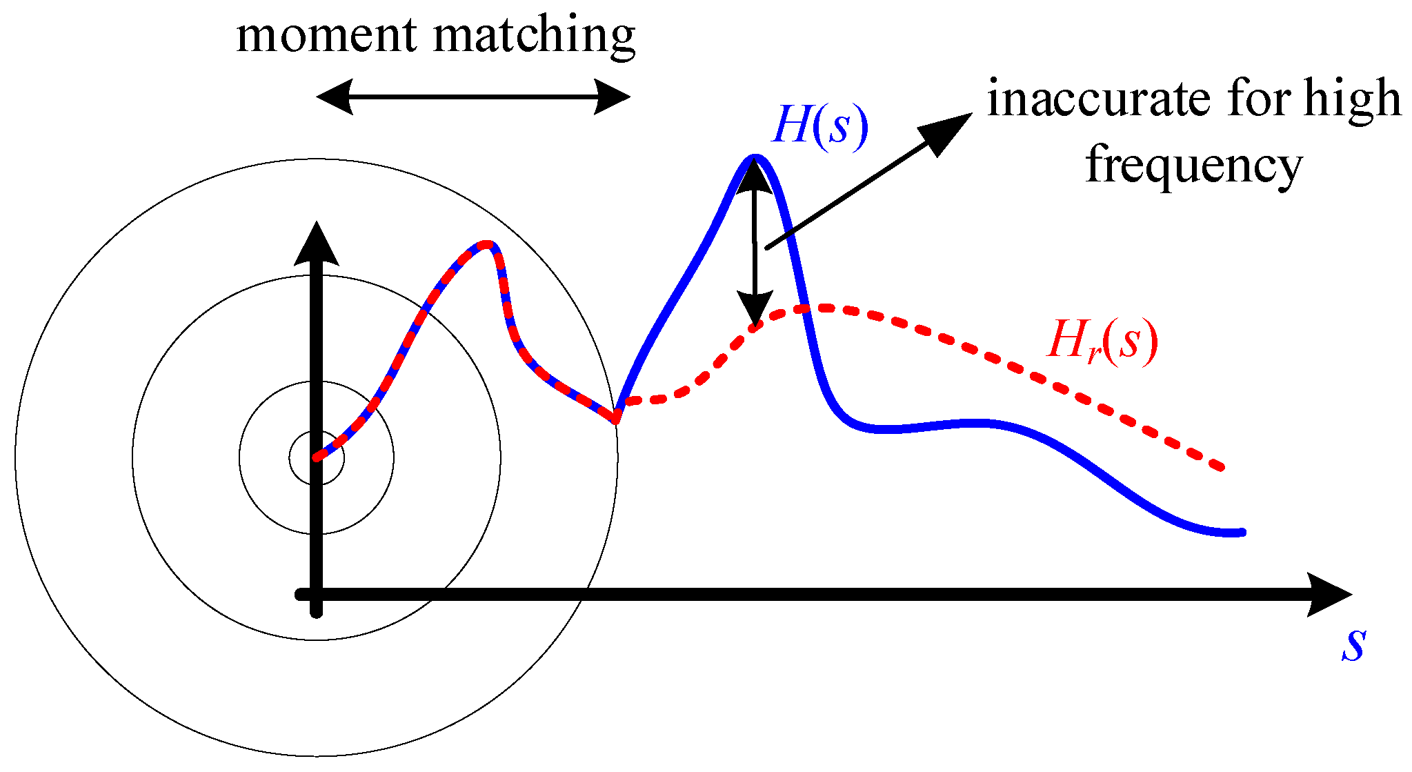
2.2. Moment Matching Method for 3-D Transient Field Problems

Moment matching is a projection-based method. In a moment-matching method, a subspace basis $V\in {\Re }^{n\times r}$ is first determined to approximate the residing manifold of the state vector, with the Petrov–Galerkin projection then used to construct the ROM. To preserve the passivity of the high-fidelity model, $W=V$ [14] is selected, yielding a reduced-order model:

$$\tilde{B}\frac{d\tilde{T}}{dt}+\tilde{A}\tilde{T}(t)=\tilde{P}J(t)$$

(3)

where, $\tilde{B}=V^{T}BV$, $\tilde{A}=V^{T}AV$, $\tilde{P}=V^{T}P$, $T=\tilde{T}{V}^T$ and $r\le n$ is the size of the reduced model (3). The matrix $V$ is computed from the following procedures. The transfer function (matrix) is

$$H(s)={(Bs+A)}^{-1}P$$

(4)

One expands $H(s)$ at point $s_0$ to

$$\begin{array}{ll}H(s)& ={(Bs+A)}^{-1}P={(B{s}_0+A+(s-s_0)B)}^{-1}P\\ & ={\displaystyle \sum _{i=0}^{+\infty }{M}_i}{(s-s_0)}^i\end{array}$$

(5)

where, $M_i={(-{(B{s}_0+A)}^{-1}A)}^i{(B{s}_0+A)}^{-1}P$, $i(0,1,2,\dots )$ is the ith moment of the system at the expansion point $s_0$. The subspace spanned by the columns of $V$ is

$$\mathrm{range}\left\{V\right\}=\mathrm{span}\left\{\widehat{P}(s_0),\left(\right(\widehat{A}(s_0){)}^{-1}A)\widehat{P}(s_0),\dots ,{\left(\right(\widehat{A}(s_0){)}^{-1}A)}^q\widehat{P}(s_0)\right\}$$

(6)

where, $\widehat{P}(s_0)={(B{s}_0+A)}^{-1}P$, $\widehat{A}(s_0)=B{s}_0+A$. In this paper, ${\left(\right(\widehat{A}(s_0){)}^{-1}A)}^i\widehat{P}(s_0)$ is the ith order moment vector.

From [14], one has

$$H_r(s)-H(s)=o{(s-s_0)}^q$$

(7)

where, $H_r(s)$ is the transfer function of the reduced model. It implies that a s₀ will guarantee that the reduced-order model achieves a relatively high accuracy of a specified frequency, with a larger q yielding a more accurate $H_r(s)$.

From (7), it is obvious that $H_r(s)$ depends also on $s_0$. For a fixed $q$, the error of $H_r$ at $s^{\prime }$ is inversely proportional to the distance of $s^{\prime }$ and $s_0$. In other words, if $s_0$ is put at zero, then $H_r(s)$ is probably not accurate at high frequencies, which is explained in detail in Figure 1.

2.3. Multipoint Expansion

The development of a feasible methodology for a wide-frequency band ROM requires compromising the accuracy of the constructed projection basis and computational cost of the procedure.

Nevertheless, a basic MOR algorithm generally employs one expansion point in developing the projection basis. However, as aforementioned, the single-point moment-matching reduced model is a locally optimal one, and it is applicable to simulating the transient response only around the frequency in question. As the frequency band of interest increases, a large number of moments need to be included to guarantee the model’s accuracy in the frequency band in question, increasing the computational and memory costs. Moreover, such a reduced model is inaccurate for simulating the transient performance of a frequency whose distance to the frequency expansion point is large. To address the locally supported approximation characteristics of a single-point moment-matching approach, the Reduced-Basis Method (RBM) [15] or Balanced Truncation Proper Orthogonal Decomposition (BT-POD) [16], based on solution snapshots [17,18] from different frequency points, is introduced. However, it involves computing snapshots on a large number of points. Moreover, for each point, a factorization operation on the system matrix is required. Consequently, such an approach considerably increases computational cost.

To take advantage of both a snapshot-based and a single-point moment-matching approach, a multipoint MOR method is developed [19,20,21,22]. A multipoint MOR method obtains the projection basis from the moments of the transfer function at multiple frequency points, as explained in Figure 2.

In [19], a fully adaptive scheme based on Krylov space was presented to reduce the size of a large-scale integrated circuit. This approach provides an interesting way of adaptively choosing expansion points by a posterior error estimation based on admittance or impedance. However, the computational process is rather complex and inefficient. Moreover, in 3-D transient field computations, the concern is more the precision or accuracy of the solution rather than the admittance or impedance parameters. Consequently, a posterior-error estimate, based on admittance or impedance, is not suitable. In [20], a greedy multipoint MOR technique chose expansion points from an arithmetic midpoint, using a posterior-error estimation based on scattering parameters, to reduce the size of a second-order electromagnetic system. In [21], an adaptive multipoint-MOR scheme, using eigen values as the stopping criterion and an error estimator, chose the new expansion point by computing error estimators at three points every time to reduce the computational cost of large-scale inductive partial element equivalent circuits (PEEC). In [22], a multipoint MOR scheme was used to reduce the size of the finite-element equation of second-order systems. The location of the expansion point and size of the projection basis were determined based on an error estimator. However, the scheme cannot be applied directly to the transient temperature problem.

In this regard, we propose a novel block Arnoldi-based multipoint-MOR scheme for 3-D transient field problems. The proposed approach not only benefits from the work of [20,21,22], but also explores the application of Krylov subspaces. The originality of this study is a novel adaptive algorithm for determining expansion points, matching moments automatically, as well as a posterior-error estimator based on the temperature response, coupled with a network topological method (NTM).

It should be noted that the optimal expansion point should be the one that gives the largest error between the current ROM and the high-fidelity model. However, finding such an ideal point is neither practical nor feasible [9]. On the other hand, although the performance of the ROM is related to the expansion point, the Krylov-based MOR is relatively insensitive to it. It is usually chosen at the point in the right-half plane whose distance to the imaginary axis is of the same magnitude as the frequency of interest [13]. From this point of view, in our application of 3-D transient field problems, the new expansion point is determined using a logarithmic scale to minimize large errors overall.

2.4. Adaptive Scheme

To start, because of the aforementioned reasons explained in 2.3, to choose the new expansion point, the logarithm midpoint is obtained from the two old expansion points as

$$f_{\mathrm{mid}}^s={10}^{(\log (f_{\min }^s)+\log (f_{\max }^s))/2}$$

(8)

where, $f_{\mathrm{mid}}^s$ denotes the midpoint frequency in logarithmic scale, with $f_{\min }^s$ and $f_{\max }^s$ denoting the minimum and maximum frequencies of the two old points, respectively.

Second, the “local error” is defined as the error between the reduced-order model (ROM) and the full model at frequency, with the “global error” as the error between the ROM and the full model over the frequency interval $[f_{\min }^{},f_{\max }^{}]$. The tolerances of the “local error” and “global errors” are initially set as $to{l}^l$ and $to{l}^g$, respectively. Moreover, one defines a posteriori-error estimator, as given in (9), to determine whether the current reduced model satisfies the accuracy requirements over a certain frequency band or only at one frequency point. Moreover,

$$E=\underset{j}{\max }\frac{{\Vert T^j(t)-T_r{}^j(t)\Vert }_2}{{\Vert T^j(t)\Vert }_2}$$

(9)

where, $T^j(t)$ and $T_r{}^j(t)$ denote the time-domain responses of the jth variable of full- and reduced-order models under an excitation signal, respectively.

Parameter $N_{\max }^{\mathrm{moments}}$ is defined as the limit of the number of moments calculated in one expansion point, and parameter $N_{\max }^s$ as the limit of the number of total expansion points used in the MOR procedure. The larger the number of moments at one frequency, the smaller the error between the ROM and the full model at this frequency is. Therefore, once the error of a frequency is smaller than the predefined tolerance, the algorithm stops moment matching at this frequency. In other words, $N_{\max }^{\mathrm{moments}}$ is equal to the smallest number of moments under which the error between the ROM and the full model is smaller than the tolerance at the frequency. Moreover, if the actual number of the expansion points used is larger than $N_{\max }^s$, the tolerance of the “local error” ($to{l}^l$) is reduced.

To facilitate the implementation of the proposed scheme, it is explained step by step as follows.

An expansion point is first chosen (here we choose $s_1^{}=f_{\min }^{}$). The moment-matching procedure at $s_1^{}$ is then activated sequentially until the local error between the ROM and the full model at frequency $f_{\min }^{}$ is smaller than the predefined tolerance. The global error (E over the frequency interval $[f_{\min }^{},f_{\max }^{}]$) checking procedure is then followed. If the error is $E<to{l}^g$, the algorithm stops and outputs the reduced model; otherwise $f_{\max }^{}$ is selected as the second expansion point. The moment-matching producer is repeated for $f_{\max }^{}$ until the “local error” between the ROM and the high fidelity model is smaller than the tolerance, and the subsequent block moments are aggregated to the basis formed by the previous ones, with an orthogonal normalization then performed to compress the projection basis. The global error E, between the ROM and high-fidelity model over the frequency interval $[f_{\min }^{},f_{\max }^{}]$, is then checked. If the error is $E<tol$, the algorithm stops and outputs the reduced-model; otherwise a middle frequency point $f_{\mathrm{mid}}^{}$ is determined by (8), between $f_{\min }^{}$ and $f_{\max }^{}$ selected as the third expansion point. For convenience of explanation, the serial numbers of ①, ③, ② are used to represent $f_{\min }^{}$, $f_{\mathrm{mid}}^{}$, and $f_{\max }^{}$, respectively. Since the moments at $f_{\min }^{}$, $f_{\mathrm{mid}}^{}$, and $f_{\max }^{}$ have already been added to the subspace of the projection basis, the next expansion point added to the subspace is chosen at the middle point between ①, ③ ($f_{\min }^{}$, $f_{\mathrm{mid}}^{}$) by Equation (8), with the serial number of the new point marked as ①-③. If the transformation matrix constructed by ①, ①-③, ③, and ② does not satisfy the accuracy tolerance, a new point is chosen, i.e., the middle point between ③ and ②, with the serial number of the new point marked as ③-②. It can be seen that the middle point between every two adjacent points is used, with the serial numbers corresponding to the points as {①, ①-③, ③, ③-②, ②}. If the error is still larger than tol^g, the middle point between every two adjacent points is chosen, i.e., the middle point between ① and ①-③, ①-③ and ③, ③and ③-②, and ③-② and ②. The iterative procedure is repeated until the error is smaller than the predefined value.

Moreover, an orthogonalization operation is applied to the so-far generated projection basis to minimize its size by discarding its redundant vectors. Although the orthogonalization and compression procedures increase computational cost, a significant improvement in performances is obtained in the projection size and reliability of the whole reduction process.

Algorithms 1–3 give the pseudocodes of the proposed MOR methodology. Algorithm 1 is the main loop of the proposed MOR scheme for 3-D transient field problems. Algorithm 2 gives the block–Arnoldi-based moment-matching methodology at a single frequency point. Algorithm 3 presents the error estimator used in the scheme.

The new Krylov subspace, a combination of the different subspaces for each expansion point, is formulated as

$$\begin{array}{ll}{U}_m& =\mathrm{span}\{\underset{\mathrm{point}s=s_1}{\underbrace{\widehat{P}(s_1),\left(\right(\widehat{A}(s_1){)}^{-1}A)\widehat{P}(s_1),\dots ,{\left(\right(\widehat{A}(s_1){)}^{-1}A)}^{q_1}\widehat{P}(s_1)}},\\ & \cdots \underset{\mathrm{point}s=s_k}{\underbrace{\widehat{P}(s_k),\left(\right(\widehat{A}(s_k){)}^{-1}A)\widehat{P}(s_k),\dots ,{\left(\right(\widehat{A}(s_k){)}^{-1}A)}^{q_k}\widehat{P}(s_k)}}\}\\ & =\mathrm{span}\left\{s_1,s_2,\cdots ,s_k\right\}\end{array}$$

(10)

where, $s_1,\cdots ,s_k$ are the expansion points used to obtain the ROM, and $q_1,\cdots q_k$ are the number of moments matched at the corresponding expansion point.

Algorithm 1. Main loop of the proposed scheme for 3-D transient field problems

Input: The range of the broadband frequency ($f_{\min }^{}$,$f_{\max }^{}$), coefficient matrices of NTM     model ($A$,$B$,$P$), global error tolerance tolg and local error tolerance toll.

1. $f_s=f_{\min }$ 2. [$Q_0$] = S-POINT ($f_s$, toll) 3. $erro{r}^g=EST-ERROR(f_{\min }^{},f_{\max }^{},Q_0,A,B,P)$ 4. while $erro{r}^g>to{l}^g$ do $f_s\leftarrow \mathrm{set}\mathrm{new}\mathrm{expansion}\mathrm{point}$ $N_s\leftarrow N_s+1$ [$Q_1$] = S-POINT ($f_s$, toll) 5. end while 6. $\tilde{A}=Q_0{}^{T}A{Q}_0$,$\tilde{B}=Q_0{}^{T}B{Q}_0$,$\tilde{P}=Q_0{}^{T}P$ Output: The coefficient matrices of a reduced system($\tilde{A}$,$\tilde{B}$,$\tilde{P}$)

Algorithm 2. S-POINT: Block Arnoldi-based moment matching at a single frequency point

Input: The current expansion point $f_s$, local error tolerance toll and coefficient matrices     of the high-fidelity model ($\tilde{A}$,$\tilde{B}$,$\tilde{P}$)

1. $r=1$ 2. $s=f_s$ 3. while $erro{r}^l>to{l}^l$ do $Q_0=blockArnoldi(s,r,A,B,P)$ $erro{r}^l$ = EST-ERROR ($f_s$,$Q_0$,A,B,P) $r\leftarrow r+1$ 4. end while Output: $Q_0$

Algorithm 3. EST-ERROR: Error estimator

Input: $Q_0$,$A$, $B$,$P$, local error: the single frequency point $f_s$, global error, the range of     the broadband frequency ($f_a^{}$,$f_b^{}$)

1. $\tilde{A}=Q_0{}^{T}A{Q}_0$,$\tilde{B}=Q_0{}^{T}B{Q}_0$,$\tilde{P}=Q_0{}^{T}P$ 2. Local error:      $f=f_s$ $J(t)=0.5\times \sin (2\pi ft)$ Get $T$ from Equation (1) under $A$, $B$, $P$ Get $T_1$ from Equation (3) under $\tilde{A}$, $\tilde{B}$, $\tilde{P}$ $\epsilon =\max \left\{\Vert T-T_1\Vert /\Vert T\Vert \right\}$ 3. Global error:        $f_k=f_a:\mathsf{\Delta }f:f_b$ $J(t)={\displaystyle \sum _{k}0.5\times \sin (2\pi f_{k}t)}$ Get $T$ from Equation (1) under $A$, $B$, $P$ Get $T_1$ from Equation (3) under $\tilde{A}$, $\tilde{B}$, $\tilde{P}$ $\epsilon =\max \left\{\Vert T-T_1\Vert /\Vert T\Vert \right\}$ 4. $error=\max \epsilon$ Output: error

3. Numerical Application

The proposed scheme and model are used to compute the transient temperature fields of a prototype insulated-gate bipolar transistor (IGBT) module (Figure 3a) to validate its advantages. The temperature field is computed by the network topological approach [23]. Figure 3b shows meshes of the NTM for the prototype IGBT module. In the numerical implementation of NTM, the numbers of the total elements and nodes are, respectively, 3364 and 4303, with the number of the NTM equations equal to 4303. Obviously, the solution of such a large equation set will consume an enormous amount of computational resources.

To simulate the wide-frequency-band transient response, the frequency broadband of excitation signals consisted of 100 liner-spaced samples from 10 Hz to 100 kHz. For performance comparisons, the NTM, the proposed reduced model and the conventional block–Arnoldi reduced model are used to compute the transient temperature field of this case study under the predefined, tested broadband excitation signal. In order to take both the minimum and maximum frequencies into consideration, the time step should be small enough and the total excitation time large enough. Consequently, the total excitation time was set as 0.2 s, the discrete number as 80,000 and the time step as 2.5 us. The equation was solved by ode15 s of MATLAB. In the solver settings, the relative tolerance (RelTol) was set as 10⁻³ and the absolute tolerance (AbsTol) as 10⁻⁶. The final expansion points used were: 10, 10⁵, 10³, and 10². As explained in the adaptive scheme, $N_{\max }^{\mathrm{moments}}$ is equal to the smallest number of moments under which the error between the ROM and the full model is smaller than the tolerance at the frequency. $N_{\max }^{\mathrm{moments}}$, at 10, 10⁵, 10³, and 10², is finally set as 6, 6, 7, and 9, respectively. Finally, $N_{\max }^s$ is set as 100 to limit the number of total expansion points used in the MOR procedure. Moreover, the local error tolerance tol^l is set as 0.005, with the global error tolerance set as 0.01. Typical observing points (points 1, 2, and 3, see Figure 3b) are used for performance comparison of different ROMs. The numerical results are presented in Figure 4, Figure 5, Figure 6, Figure 7, Figure 8 and Figure 9.

Figure 4, Figure 5 and Figure 6 present the time-domain response observed on points 1, 2, and 3 of the NTM model and those of the proposed reduced model (size = 28), respectively. From the numerical results, it is obvious that the proposed reduced-order system can accurately imitate the dynamic response of the original high-fidelity model. Moreover, Figure 7, Figure 8 and Figure 9 provide the absolute errors observed on points 1, 2, and 3, between the results of the NTM model and those of the proposed reduced model (size = 28), and those of the conventional block–Arnoldi reduced model (size = 30), respectively. From the numerical results (Figure 7, Figure 8 and Figure 9), one can see that for a dynamic response to a broadband frequency signal, the absolute transient errors of the proposed model are much smaller than those for the conventional reduced model. For point 1, the maximum error of the proposed model is 0.3603, whereas the conventional reduced model can reach 3.2275. For point 2, the maximum error of the proposed approach is 0.0986, whereas the conventional reduced model can reach 0.9803. For point 3, the maximum error of the proposed model is 0.1459, whereas the conventional reduced model can reach 6.3752. More performance comparison statistics are shown in

Table 1. Comparisons of the transient response on different observing points by using the proposed and NTM models.

Analysis Point	NTM Model		Proposed
	max (K)	min (K)	max (K)	min (K)
Point 1	40.9190	−37.1739	40.9114	−37.1928
Point 2	12.3376	−9.8100	12.3112	−9.8353
Point 3	19.9404	−17.9279	19.9244	−17.9785

and

Table 2. Comparisons of the absolute errors on different observing points by using the proposed and conventional schemes.

Analysis Point	Block Arnoldi (Order = 30)			Proposed (Order = 28)
	max (K)	min (K)	Average (K)	max (K)	min (K)	Average (K)
Point 1	3.2275	0	0.1869	0.3603	0	0.0689
Point 2	0.9803	0	0.0543	0.0986	0	0.0246
Point 3	6.3752	0	0.1995	0.1459	0	0.0224

. Table 1 compares the transient response of different observing points using the proposed and NTM models. Table 2 compares the absolute errors on different observing points using the proposed and conventional schemes. The numerical results in Table 1 and Table 2 also validate the conclusion obtained from Figure 4, Figure 5, Figure 6, Figure 7, Figure 8 and Figure 9.

Table 3. Comparisons of relative errors on different observing points by using the proposed and conventional schemes.

Analysis Point	Proposed (Order = 28)	Block Arnoldi (Order = 20)	Block Arnoldi (Order = 30)
Point 1	0.0066	0.0479	0.0246
Point 2	0.0065	0.0298	0.0190
Point 3	0.0088	0.2659	0.1627

gives the relative errors (norm-2 error) computed by Equation (9) on points 1, 2, and 3 of the results of the NTM model, those of the proposed reduced model (size = 28), those of the conventional block-Arnoldi reduced model (size = 20) and those of the conventional block-Arnoldi reduced model (size = 30). From the numerical results of the two conventional ROMs, it is easy to observe that a high-order reduced model produces a more accurate result compared to a low-order one. However, the high-order conventional reduced model is less accurate than the proposed one, which validates the merits of the proposed ROM scheme.

Moreover, the time discretization time for all models is 80,000. For the NTM model of the prototype IGBT, the CPU times for a transient process are 64,436.92 s, while those for the proposed model are 8038.95 s. The CPU times for implementing the proposed scheme are about 35 s; the total used by the proposed model for the same transient simulations (8073.95 s) is less than 13% of those of the original NTM.

4. Conclusions

To increase the computational speed of a high-fidelity model in solving a complex 3-D transient field problem by a numerical approach, a block Arnoldi-based multipoint-model order-reduction scheme is presented. The proposed methodology was used to reduce the size of an NTM high-fidelity model in solving the three-dimensional temperature field of a case study. The computational results have demonstrated:

(1)

The model reduced from the proposed methodology could achieve a higher accuracy compared to one reduced from conventional block Arnoldi in a wideband frequency. For point 1, the maximum error of the proposed model was 0.3603, whereas that of the conventional reduced model can reach 3.2275. For point 2, the maximum error of the proposed approach is 0.0986, whereas that of the conventional reduced model can reach 0.9803. For point 3, the maximum error of the proposed model is 0.1459, whereas that of the conventional reduced model can reach 6.3752.

(2)

The ROM obtained using the proposed scheme can accurately replicate the transient temperature fields of the NTM high-fidelity model through a wide frequency range, while the computational time of the reduced-order model is less than 13% of the original one.

It should be noted that an MOR method is generally applicable to a linear system. However, for a nonlinear system, a linearization technique must first be implemented in the system before the application of an MOR. Additionally, once the proposed ROM has been learned in the offline stage, it can be used to simulate a transient response of the system for any excitation J(t), as long as its frequency spectrum stays in the learned-frequency interval.

References

1. Necoara, I.; Ionescu, T.C. H2 Model Reduction of Linear Network Systems by Moment Matching and Optimization. IEEE Trans. Autom. Control 2020, 65, 5328–5335. [Google Scholar] [CrossRef] [Green Version]
2. Mohamed, K. Model Order Reduction Method for Large-Scale RC Interconnect and Implementation of Adaptive Digital PI Controller. IEEE Trans. Very Large Scale Integr. VLSI Syst. 2019, 27, 2447–2458. [Google Scholar] [CrossRef]
3. Farhan, M.A.; Nakhla, M.S. Parametric Order Reduction of Nonuniform Interconnect Circuits Using Integrated Congruence Transform. IEEE Trans. Compon. Packag. Manufact. Technol. 2018, 8, 1956–1966. [Google Scholar] [CrossRef]
4. Szypulski, D.; Fotyga, G.; Rubia, V.; Mrozowski, M. A Subspace-Splitting Moment-Matching Model-Order Reduction Technique for Fast Wideband FEM Simulations of Microwave Structures. IEEE Trans. Microw. Theory Tech. 2020, 68, 3229–3241. [Google Scholar] [CrossRef]
5. Fotyga, G.; Nyka, K.; Mrozowski, M. Automatic Reduction-Order Selection for Finite-Element Macromodels. IEEE Microw. Compon. Lett. 2018, 28, 278–280. [Google Scholar] [CrossRef]
6. Kuriyama, K.; Kameari, A.; Ebrahimi, H.; Fujiwara, T.; Sugahara, K.; Shindo, Y.; Matsuo, T. Cauer Ladder Network With Multiple Expansion Points for Efficient Model Order Reduction of Eddy-Current Field. IEEE Trans. Magn. 2019, 55, 1–4. [Google Scholar] [CrossRef]
7. Sakamoto, H.; Okamoto, K.; Igarashi, H. Fast Analysis of Rotating Machine Using Simplified Model-Order Reduction Based on POD. IEEE Trans. Magn. 2020, 56, 1–4. [Google Scholar] [CrossRef] [Green Version]
8. Sanaie, R.; Chiprout, E.; Nakhla, M.S.; Zhang, Q. A fast method for frequency and time domain simulation of high speed VLSI interconnects. IEEE Trans. Microw. Theory Tech. 1994, 42, 2562–2571. [Google Scholar] [CrossRef]
9. Feldmann, P.; Freund, R.W. Efficient linear circuit analysis by Padé approximation via the Lanczos Process. IEEE Trans. Comput. Aided Des. Integr. Circuits Syst. 1995, 14, 639–649. [Google Scholar] [CrossRef]
10. Slone, R.D. Removing the frequency restriction on Padé via Lanczo with an error bound. In Proceedings of the 1998 IEEE International Symposium on Electromagnetic Compatibility. Part 1 (of 2), Denver, CO, USA, 24–28 August 1998; pp. 202–207. [Google Scholar]
11. Bai, Z.; Slone, R.D.; Smith, W.T.; Ye, Q. Error bound for reduced system model by Padé approximation via the Lanczos process. IEEE Trans. Comput. Aided Des. Integr. Circuits Syst. 1999, 18, 133–141. [Google Scholar]
12. Chen, J.; Hu, S.; Zhou, Q.; Yang, S.; Ren, Z. A Broadband Enhanced Nodal-Order Reduction Methodology for Large-Scale Equation Sets of 3-D Transient Field Problems. IEEE Trans. Magn. 2020, 56, 1–4. [Google Scholar] [CrossRef]
13. Schilders, W.H.A.; van der Vorst, H.A.; Rommes, J. Model Order Reduction: Theory, Research Aspects and Applications, 1st ed.; Springer: Berlin/Heidelberg, Germany, 2008; pp. 60–70. [Google Scholar]
14. Odabasioglu, A.; Celik, M.; Pileggi, L.T. PRIMA: Passive reducedorde interconnect macromodeling algorithm. IEEE Trans. Comput. Aided Des. Integr. Circuits Syst. 1998, 17, 645–654. [Google Scholar] [CrossRef] [Green Version]
15. Rubia, V.D.L.; Razafison, U.; Maday, Y. Reliable fast frequency sweep for microwave devices via the reduced-basis method. IEEE Trans. Microw. Theory Tech. 2009, 57, 2923–2937. [Google Scholar] [CrossRef] [Green Version]
16. Wang, W.; Paraschos, G.N.; Vouvakis, M.N. Fast frequency sweep of FEM models via the balanced truncation proper orthogonal decomposition. IEEE Trans. Antennas Propag. 2011, 59, 4142–4154. [Google Scholar] [CrossRef]
17. Xu, B.; Yebi, A.; Hoffman, M.; Onori, S. A Rigorous Model Order Reduction Framework for Waste Heat Recovery Systems Based on Proper Orthogonal Decomposition and Galerkin Projection. IEEE Trans. Control Syst. Technol. 2020, 28, 635–643. [Google Scholar] [CrossRef]
18. Kasolis, F.; Clemens, M. Entropy Snapshot Filtering for QR-Based Model Reduction of Transient Nonlinear Electro-Quasi-Static Simulations. IEEE Trans. Magn. 2020, 56, 1–4. [Google Scholar] [CrossRef]
19. Feng, L.; Korvink, J.G.; Benner, P. A Fully Adaptive Scheme for Model Order Reduction Based on Moment Matching. IEEE Trans. Compon. Packag. Manufact. Technol. 2015, 5, 1872–1884. [Google Scholar] [CrossRef]
20. Rewienski, M.; Lamecki, A.; Mrozowski, M. Greedy Multipoint Model-Order Reduction Technique for Fast Computation of Scattering Parameters of Electromagnetic Systems. IEEE Trans. Microw. Theory Tech. 2016, 64, 1681–1693. [Google Scholar] [CrossRef]
21. Nguyen, T.; Duc, T.L.; Tran, T.; Guichon, J.; Chadebec, O.; Meunier, G. Adaptive Multipoint Model Order Reduction Scheme for Large-Scale Inductive PEEC Circuits. IEEE Trans. Electromagn. Compat. 2017, 59, 1143–1151. [Google Scholar] [CrossRef]
22. Fotyga, G.; Czarniewska, M.; Lamecki, A.; Mrozowski, M. Reliable Greedy Multipoint Model-Order Reduction Techniques for Finite-Element Analysis. IEEE Antennas Wirel. Propag. Lett. 2018, 17, 821–824. [Google Scholar] [CrossRef]
23. Chen, J.; Yang, S.; Ren, Z. A Network Topological Approach-Based Transient 3-D Electrothermal Model of Insulated-Gate Bipolar Transistor. IEEE Trans. Magn. 2020, 56, 1–4. [Google Scholar] [CrossRef]
Figure 1. Taylor expansion around s = 0.
Applsci 11 09435 g001
Figure 2. Taylor expansion around several points.
Applsci 11 09435 g002
Figure 3. Prototype (a) IGBT module and its (b) NTM model.
Applsci 11 09435 g003
Figure 4. Time-domain transient response on point 1. (a) Zoom in (0–0.12 s). (b) Whole excitation duration (0–0.2 s).
Applsci 11 09435 g004
Figure 5. Time-domain transient response on point 2. (a) Zoom in (0–0.12 s). (b) Whole excitation duration (0–0.2 s).
Applsci 11 09435 g005
Figure 6. Time-domain transient response on point 3. (a) Zoom in (0–0.12 s). (b) Whole excitation duration (0–0.2 s).
Applsci 11 09435 g006
Figure 7. Absolute errors of the computed temperatures observing point 1, using the conventional block Arnoldi algorithm and the proposed scheme, compared to those of the original NTM model under the tested broad-frequency-excitation signal. (a) Zoom in (0–0.12 s). (b) Whole excitation duration (0–0.2 s).
Applsci 11 09435 g007
Figure 8. Absolute errors of the computed temperatures on observing point 2, using the conventional block Arnoldi algorithm and the proposed scheme, compared to those of the original NTM model under the tested broad-frequency-excitation signal. (a) Zoom in (0–0.12 s). (b) Whole excitation duration (0–0.2 s).
Applsci 11 09435 g008
Figure 9. Absolute errors of the computed temperatures on observing point 3, using the conventional block Arnoldi algorithm and the proposed scheme, compared to those of the original NTM model under the tested broad-frequency-excitation signal. (a) Zoom in (0–0.12 s). (b) Whole excitation duration (0–0.2 s).
Applsci 11 09435 g009