Cardiac Arrhythmia Classification Based on One-Dimensional Morphological Features

Featured Application

Authors are encouraged to provide a concise description of the specific application or a potential application of the work. This section is not mandatory.

Abstract

The electrocardiogram (ECG) is the most commonly used tool for diagnosing cardiovascular diseases. Recently, there have been a number of attempts to classify cardiac arrhythmias using machine learning and deep learning techniques. In this study, we propose a novel method to generate the gray-level co-occurrence matrix (GLCM) and gray-level run-length matrix (GLRLM) from one-dimensional signals. From the GLCM and GLRLM, we extracted morphological features for automatic ECG signal classification. The extracted features were combined with six machine learning algorithms (decision tree, k-nearest neighbor, naïve Bayes, logistic regression, random forest, and XGBoost) to classify cardiac arrhythmias. Experiments were conducted on a 12-lead ECG database collected from Chapman University and Shaoxing People’s Hospital. Of the six machine learning algorithms, combining XGBoost with the proposed features yielded an accuracy of 90.46%, an AUC of 0.982, a sensitivity of 0.892, a precision of 0.900, and an F1 score of 0.895 and presented better results than wavelet features with XGBoost. The experimental results show the effectiveness of the proposed feature extraction algorithm.

1. Introduction

Cardiovascular diseases (CVDs) are the leading cause of death worldwide. About 17.9 million people died from CVDs in 2019, accounting for 32% of global deaths. Of these, 85% died from heart attacks and strokes [1]. CVDs contain an irregular rhythm of the heartbeat and affect the electrical system of the heart. Therefore, early and accurate detection of the irregular rhythm of the heartbeat is an important clinical task to prevent death from CVDs. The electrocardiogram (ECG), which records the electrical activity passing through the heart non-invasively, is one of the most used clinical tools to diagnose cardiac function. In particular, a standard short-duration 12-lead ECG system is employed from primary clinics to intensive care units since it can provide a complete evaluation of the cardiac electrical activity, such as arrhythmias, conduction disturbances, acute coronary syndromes, and cardiac chamber hypertrophy and enlargement [2]. Interpretation of ECG signals is usually conducted by primary care physicians, which is a tedious and time-consuming task [3]. Advanced decision support systems that rely on automatic ECG interpretation algorithms could provide primary care physicians with relevant information.

Methods for automatically interpreting ECG signals can be divided two categories: (1) feature-based methods, which use hand-crafted features; and (2) deep-learning-based methods, which automatically extract features from ECG signals. The former are mainly used in combination with conventional machine learning algorithms, and it is possible to interpret the extracted features. In contrast, the latter learn in an end-to-end manner and it is difficult to interpret features. However, they demonstrate better performance than conventional machine learning methods in classifying ECG signals when trained with a sufficient amount of data [4].

For feature-based methods, various types of morphological or statistical features manually extracted from ECG signals in the time domain, the frequency domain, or the nonlinear domain have commonly been used [5,6]. Philip de [7] extracted ECG morphologies, heartbeat intervals, and RR intervals for automated heartbeat classification systems. Sharma [8] decomposed multi-lead ECGs into different sub-bands utilizing a stationary wavelet transform and obtained features. These features were used for the detection of inferior myocardial infarction.

Deep-learning-based methods, such as convolutional neural networks (CNNs), recurrent neural networks (RNNs), and long-short term memory (LSTM), are widely applied to interpret ECG signals automatically [4,9,10] since these methods can learn inherent well-distinguishable features from raw ECG signals without relying on a cardiologist’s intervention. CNNs can effectively learn morphological features of ECG signals [11] and RNNs and LSTM can extract global time-dependent features related to time-varying dynamics through recurrent connections [12,13].

Recently, a hybrid approach using a combination of a feature-based method and a deep learning method has also been widely used. Hasan [14] fed a modified ECG formed by summing the first three intrinsic mode functions with the use of empirical mode decomposition into a one-dimensional CNN to recognize ECG signals. An approach based on a 1D canonical correlation analysis network with handcrafted features was also presented for ECG classification [15].

In this study, we propose a novel feature extraction method that focuses on morphological features of one-dimensional ECG signals. In order to extract morphological features, we adopt the gray-level co-occurrence matrix (GLCM) and the gray-level run-length matrix (GLRLM), which are widely used statistical tools for extracting texture information from images. To the best of our knowledge, there are no studies that have applied the GLCM or the GLRLM to one-dimensional signals. A large public dataset of 12-lead ECG arrhythmia signals [16] was used to verify the proposed method.

2. Materials and Methods

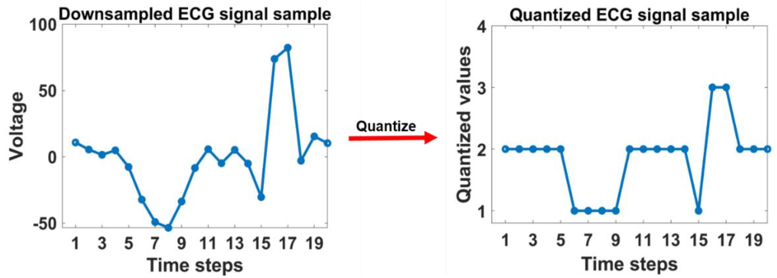
2.1. Dataset and Preprocessing

In this study, we used a 12-lead ECG database collected by Chapman University and Shaoxing People’s Hospital (Shaoxing Hospital Zhejiang University School of Medicine) to verify the validation of the proposed morphological features [16]. The 12-lead ECG database covers 10,646 patients (5956 males) and was sampled at 500 Hz over a period of 10 s. The ECG database contains 11 heart rhythms that were labeled by professional physicians. Three steps were sequentially applied to process the raw ECG signals. As the first step, a Butterworth low-pass filter was applied to reject signals with frequencies above 50 Hz since the frequency range of a normal ECG is between 0.5 Hz and 50 Hz [17]. Then, the local polynomial regression smoother (LOESS) curve fitting was utilized to remove the baseline wandering effect that could be induced by respiration [18]. Finally, the non-local means (NLMs) were applied to reduce residual noises [19]. A total of 10,588 data samples were used in this experiment because some ECG records contained only zeros and some channel values were missing. In

Table 1. Information on the 11 ECG rhythms and the four merged groups.

ECG Rhythm Names	Number of Subjects	Merged Group Names	Number of Subjects
Atrial Fibrillation (AFIB)	1780	AFIB	2218
Atrial Flutter (AF)	438
Atrial Tachycardia (AT)	121	GSVT	2260
Atrioventricular Node Reentrant Tachycardia (AVNRT)	16
Atrioventricular Reentrant Tachycardia (AVRT)	8
Sinus Atrium to Atrial Wandering Rhythm (SAAWR)	7
Sinus Tachycardia (ST)	1564
Supraventricular Tachycardia (SVT)	544
Sinus Bradycardia (SB)	3888	SB	3888
Sinus Rhythm (SR)	1825	SR	2222
Sinus Irregularity (SI)	397

, details of the 11 ECG rhythms and the corresponding number of subjects are described. Some ECG rhythms contained less than 100 samples, which can cause data imbalance issues. Thus, as suggested by Zheng [16], the 11 rhythms were hierarchically merged into four groups (AFIB, GSVT, SB, and SR). As shown in Table 1, AFIB contained atrial fibrillation (AFIB) and atrial flutter (AF). GSVT consisted of atrial tachycardia (AT), atrioventricular node reentrant tachycardia (AVNRT), atrioventricular reentrant tachycardia (AVRT), sinus atrium to atrial wandering rhythm (SAAWR), sinus tachycardia (ST), and supraventricular tachycardia (SVT). SB only included sinus bradycardia (SB). SR included sinus rhythm (SR) and sinus irregularity (SI).

For data manipulation, we rescaled the ECG signals to between 0 and 1 using a min–max algorithm to incorporate the amplitude scale and help reduce differences in gender and age effects. Then, we quantized the ECG signals to generate the GLCM and GLRLM. With the help of the Lloyd-max algorithm [20], the ECG signals were quantized into 16, 32, 64, and 128 levels. Finally, downsampling was done to reduce the computational burden. All ECG recordings were resampled to a 100 Hz sampling rate. Figure 1 shows a downsampled ECG signal and its quantized ECG signal. Preprocessing of the raw ECG signals, data manipulation, and feature extractions were implemented in Matlab 2020a (https://www.mathworks.com, accessed on 11 October 2021).

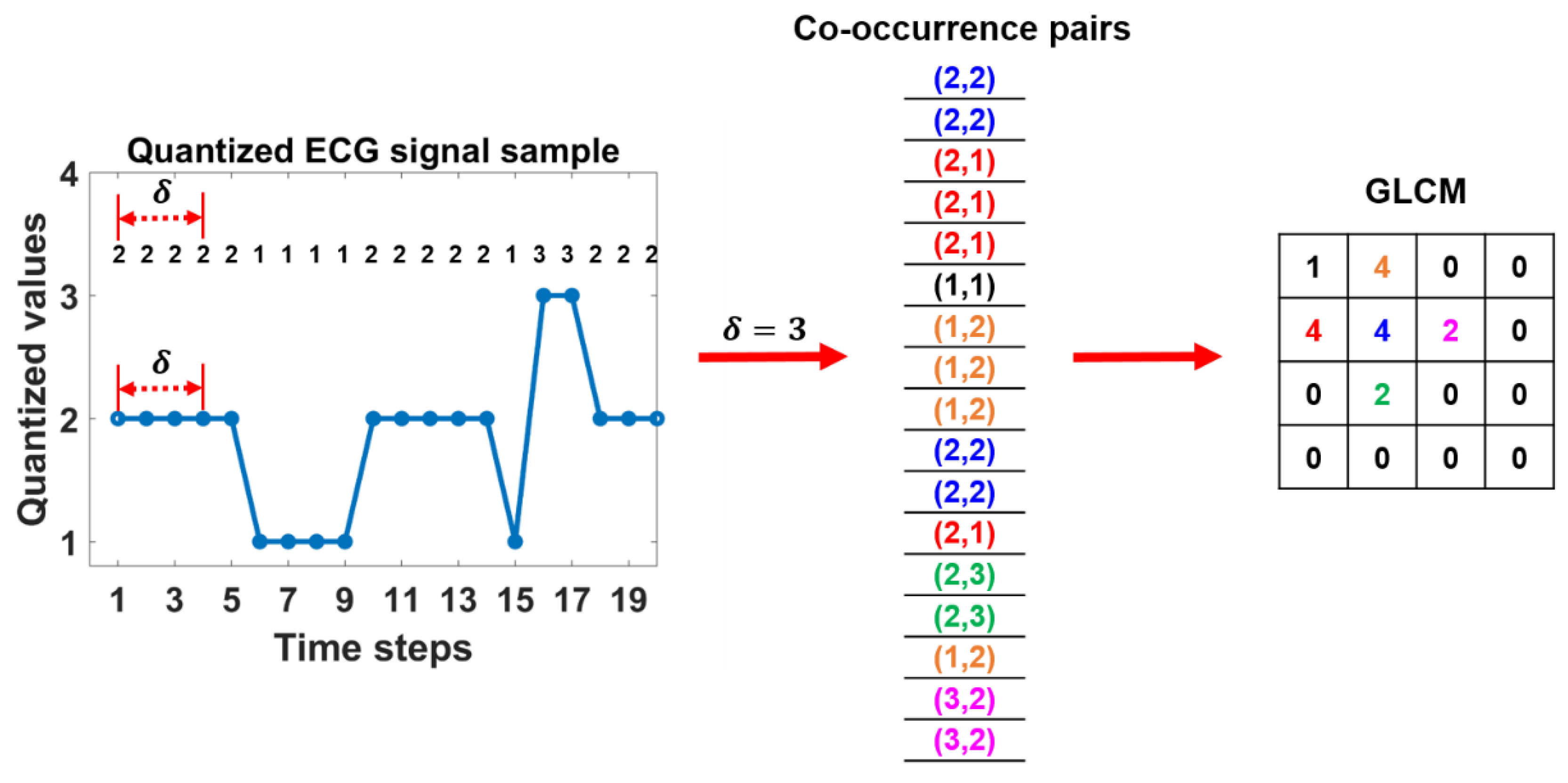
2.2. Proposed One-Dimensional Feature Extraction Method

In this study, we extracted three feature groups from one-dimensional ECG signals: first-order features, GLCM features (second-order features), and GLRLM features (higher-order features). First-order features are derived from calculating the statistical moment of the signal histogram. GLCM is a texture analysis method for computing how often pairs of pixels with specific values in a specified spatial relationship occur in an image [21]. Similarly, GLRLM quantifies gray level runs, which are defined as the length in the number of consecutive pixels that have the same gray level value in an image [22]. Both GLCM and GLRLM measure the heterogeneity and statistical characteristics of the region of interest in the image and provide an extraordinary statistical feature extraction ability. These features have been widely used for texture feature descriptors in medical fields [23,24]. GLCM and GLRLM are mainly used for images that contain two-dimensional data. Thus, GLCM and GLRLM must be redefined for one-dimensional signals. The following subsections describe how to generate the GLCM and GLRLM from one-dimensional signals.

2.2.1. First-Order Features

First-order features were calculated from the histogram of the quantized ECG signal, which represents the distribution of quantized values. When computing the histogram, the bin size must be determined. We adopted the bin size using the automatic binning algorithm provided by Matlab 2020a. From the histogram, we obtained 11 features: uniformity, energy, entropy, kurtosis, mean, mean absolute deviation, median, sum of intensities, root mean square, skewness, and standard deviation.

2.2.2. GLCM features

Let $G_{\delta }\left(i,j\right)$ denote the GLCM and represent the number of times that quantized value $i$ is neighbors with quantized value $j$ at a distance $\delta$. The GLCM has the size of $p\times p$, where $p$ describes a pre-defined number of quantized levels of the ECG signal. Both the offset distance $\delta$ and the quantized level $p$ are hyperparameters to be tuned. In this study, the offset distance $\delta$ ranges from 1 to 10 with an interval of 1 and the quantization level $p$ was chosen from 16, 32, 64, and 128 levels. Both hyperparameters were optimized by the grid search. For each ECG lead, the $p\times p$ GLCM $G_{\delta }\left(i,j\right)$ can be defined as follows:

$$G_{\delta }\left(i,j\right)={\displaystyle \sum }_{x=1}^{n-\delta }\{\begin{array}{cc}1,& if y\left(x\right)=i \& y\left(x+\delta \right)=j \\ 0,& otherwise \end{array},$$

(1)

where $y$ is a quantized ECG signal, $i$ and $j$ are the quantized values of $y$, $x$ is a temporal position of $y$, and $n$ is the end position of the quantized ECG signal. Figure 2 illustrates how to generate the GLCM when the offset distance $\delta$ is 3. After computing the GLCM, we obtained nine features (energy, contrast, entropy, homogeneity, correlation, dissimilarity, autocorrelation, average, and variance). The mathematical definition and the meaning of the features are presented in

Table 2. GLCM features. $g\left(i,j\right)$ is the normalized GLCM. $\mu$ and $\sigma$ are the mean and standard deviation of $g\left(i,j\right)$, respectively. $g_{x+y}\left(k\right)$ is obtained from ${\displaystyle \sum }_i^p{\displaystyle \sum }_j^{p}g\left(i,j\right)$ and $k=i+j$.

GLCM Feature Names	Definition	Measure
Energy	${\displaystyle \sum }_i^p{\displaystyle \sum }_j^{p}g{\left(i,j\right)}^2$	homogeneous patterns
Contrast	${\displaystyle \sum }_i^p{\displaystyle \sum }_j^p{\left(i-j\right)}^2\ast g\left(i,j\right)$	local variation, favoring values away from the diagonal ($i=j$)
Entropy	$-{\displaystyle \sum }_i^p{\displaystyle \sum }_j^{p}g\left(i,j\right)\ast lo{g}_{2}g\left(i,j\right)$	the randomness and variability in neighborhood values
Homogeneity	${\displaystyle \sum }_i^p{\displaystyle \sum }_j^p\frac{g\left(i,j\right)}{1+\left|i-j\right|}$	with more uniform levels; the denominator will remain low, resulting in a higher overall value
Correlation	$\frac{1}{\sigma }{\displaystyle \sum }_i^p{\displaystyle \sum }_j^p\left(i-\mu \right)\left(j-\mu \right)\ast g\left(i,j\right)$	linear dependency of quantized values on their respective signals in the GLCM
Dissimilarity	${\displaystyle \sum }_i^p{\displaystyle \sum }_j^p\left|i-j\right|\ast g\left(i,j\right)$	local intensity variation defined as the mean absolute difference between the neighboring pairs
Autocorrelation	${\displaystyle \sum }_i^p{\displaystyle \sum }_j^{p}i\ast j\ast g\left(i,j\right)$	magnitude of the fineness and coarseness of the texture
Sum average	${\displaystyle \sum }_k^{2p}i\ast g_{x+y}\left(k\right)$	relationship between occurrences of pairs with lower values and occurrences of pairs with higher values
Variance	${\displaystyle \sum }_i^p{\displaystyle \sum }_j^p{\left(i-\mu \right)}^{2}g\left(i,j\right)$	groupings of signals with similar quantized values

[25].

2.2.3. GLRLM Features

The GLRLM is also generated from a quantized ECG signal. Let $Q\left(i,j\right)$ denote the GLRLM and represent the number of runs of quantized value $i$ with $j$ consecutive quantized values. The GLRLM has the size of $p\times q$, where $p$ describes a pre-defined number of quantized levels and $q$ represents the length of the longest run of quantized gray level sets in the ECG signal. Figure 3 briefly depicts the process of generating the GLRLM. From the GLRLM, we can extract 13 features (short run emphasis, long run emphasis, gray-level nonuniformity, run-length nonuniformity, run percentage, low gray-level run emphasis, high gray-level run emphasis, short run low gray-level emphasis, short run high gray-level emphasis, long run low gray-level emphasis, long run high gray-level emphasis, gray-level variance, and run-length variance) as presented in

Table 3. GLRLM features. $Q\left(i,j\right)$ is the GLRLM representing the number of runs of quantized gray level $i$ and consecutive length $j$. $N_{run}$ is the number of runs of the GLRLM and $N_p$ is the total signal length. ${\mu }_i={\displaystyle \sum }_i^p{\displaystyle \sum }_j^{q}i\ast \frac{Q\left(i,j\right)}{N_{run}}$ and ${\mu }_j={\displaystyle \sum }_i^p{\displaystyle \sum }_j^{q}j\ast \frac{Q\left(i,j\right)}{N_{run}}$.

GLRLM Feature Names	Definition	Measure
Short Run Emphasis	$\frac{1}{N_{run}}{\displaystyle \sum }_i^p{\displaystyle \sum }_j^q\frac{1}{j^2}\ast Q\left(i,j\right)$	distribution of short run lengths
Long Run Emphasis	$\frac{1}{N_{run}}{\displaystyle \sum }_i^p{\displaystyle \sum }_j^q{j}^2\ast Q\left(i,j\right)$	distribution of long run lengths
Gray-Level Nonuniformity	$\frac{1}{N_{run}}{\displaystyle \sum }_i^p{\left({\displaystyle \sum }_j^{q}Q\left(i,j\right)\right)}^2$	similarity of quantized values in the signal
Run-Length Nonuniformity	$\frac{1}{N_{run}}{\displaystyle \sum }_j^q{\left({\displaystyle \sum }_i^{p}Q\left(i,j\right)\right)}^2$	similarity of run lengths throughout the signal
Run Percentage	$\frac{N_{run}}{N_p}$	coarseness of the signal
Low Gray-Level Run Emphasis	$\frac{1}{N_{run}}{\displaystyle \sum }_i^p{\displaystyle \sum }_j^q\frac{1}{i^2}\ast Q\left(i,j\right)$	distribution of the lower quantized values
High Gray-Level Run Emphasis	$\frac{1}{N_{run}}{\displaystyle \sum }_i^p{\displaystyle \sum }_j^q{i}^2\ast Q\left(i,j\right)$	distribution of the higher quantized values
Short Run Low Gray-Level Emphasis	$\frac{1}{N_{run}}{\displaystyle \sum }_i^p{\displaystyle \sum }_j^q\frac{1}{i^2\ast j^2}\ast Q\left(i,j\right)$	joint distribution of shorter run lengths with lower quantized values
Short Run High Gray-Level Emphasis	$\frac{1}{N_{run}}{\displaystyle \sum }_i^p{\displaystyle \sum }_j^q\frac{i^2}{j^2}\ast Q\left(i,j\right)$	joint distribution of shorter run lengths with higher quantized values
Long Run Low Gray-Level Emphasis	$\frac{1}{N_{run}}{\displaystyle \sum }_i^p{\displaystyle \sum }_j^q\frac{j^2}{i^2}\ast Q\left(i,j\right)$	joint distribution of long run lengths with lower quantized values
Long Run High Gray-Level Emphasis	$\frac{1}{N_{run}}{\displaystyle \sum }_i^p{\displaystyle \sum }_j^q{i}^2\ast j^2\ast Q\left(i,j\right)$	joint distribution of long run lengths with higher quantized values
Gray-Level Variance	${\displaystyle \sum }_i^p{\displaystyle \sum }_j^q{\left(i-{\mu }_i\right)}^2\ast \frac{Q\left(i,j\right)}{N_{run}}$	variance in gray level intensity for the runs
Run-Length Variance	${\displaystyle \sum }_i^p{\displaystyle \sum }_j^q{\left(j-{\mu }_j\right)}^2\ast \frac{Q\left(i,j\right)}{N_{run}}$	variance in runs for the run lengths

[25].

2.3. Wavelet Features

To verify the validity of the morphological features proposed in this study, comparisons were made using statistical features obtained from wavelet coefficients, which are often used to classify cardiac arrhythmias [8]. Wavelets are a popular tool for computational harmonic analysis, providing localization in both the temporal (or spatial) domain and the frequency domain [26]. The wavelet features were extracted for each lead using a multi-level (five-level) 1-D discrete wavelet transform (Daubechies db6) for each lead independently [26]. From the resulting coefficients, we obtained various statistical features, including the 5th, 25th, 75th, and 95th percentiles, median, mean, standard deviation, variance, root of squared means, and number of zero and mean crossings, as suggested in [26,27].

2.4. Machine Learning

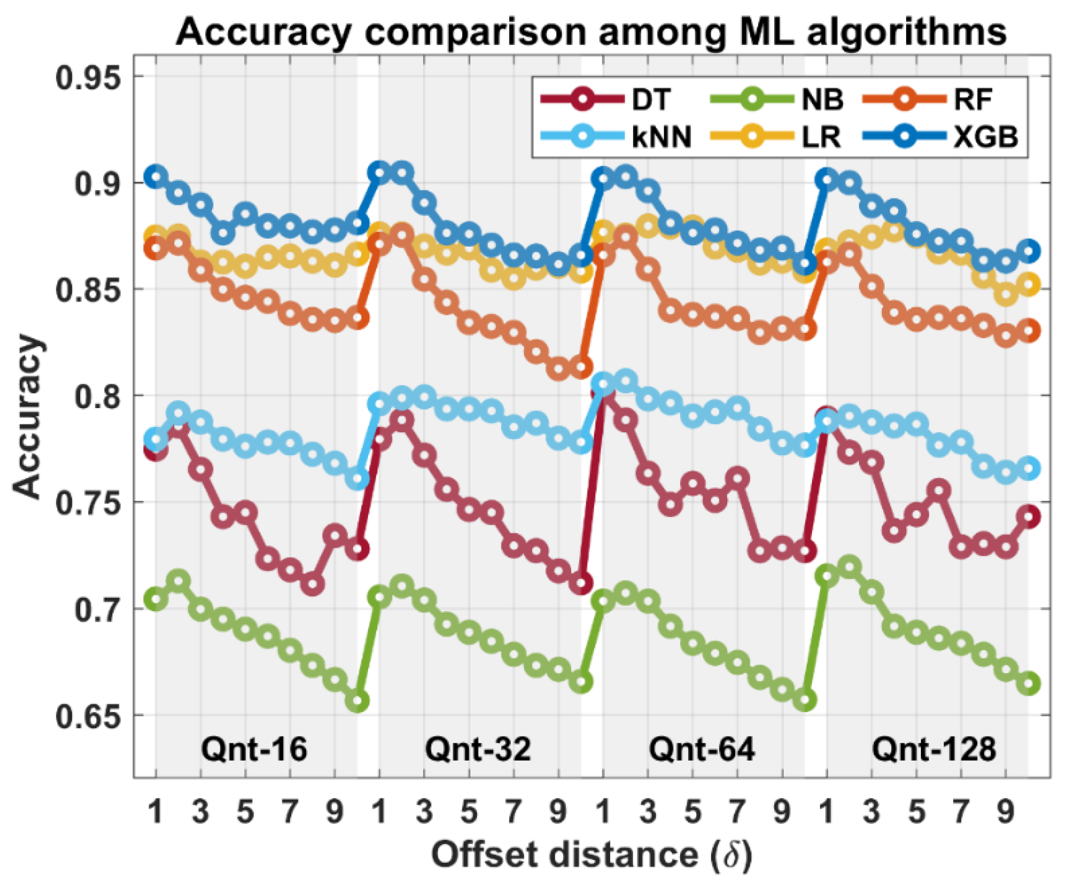
For each ECG lead, we extracted 11 first-order features, 9 GLCM features, and 13 GLRLM features. A total of 33 features were extracted from a single ECG lead. Since we dealt with 12-lead ECG signals, the total number of extracted features was 396 features for each subject. Before applying the morphological features of the 1D signal to the machine learning algorithms, we randomly split the feature sets into a training subset (n = 6776, 64%), a validation subset (n = 1694, 16%), and a test subset (n = 2118, 20%) for 5-fold cross-validation.

In this study, we investigated six machine learning classifiers (decision tree (DT), k-nearest neighbor (kNN), naïve Bayes (NB), random forest (RF), logistic regression (LR), and XGBoost (XGB)). All classifiers were implemented using Scikit-learn (https://scikit-learn.org, accessed on 11 October 2021), which provides a user-friendly interface for accessing many machine learning algorithms in Python. During the training phase, machine learning algorithms use training subsets to train the models’ weights and employ validation subsets to optimize models’ hyperparameters. The optimal hyperparameters were selected based on the accuracy and obtained through a comprehensive grid search. Information on the hyperparameters that were tuned by a grid search is provided in

Table 4. Hyperparameters. DT, decision tree; kNN, k-nearest neighbor; NB, naïve Bayes; RF, random forest; LR, logistic regression; XGB: XGBoost. In the naïve Bayes (NB) classifier, no hyperparameter was used.

Classifier	Hyperparameters in Scikit-Learn	Hyperparameter Grid
DT	max_depth	2, 4, 6, 8, 10, 12, 14, 16, 18, 20, None
kNN	n_neighbors	5, 7, 9, 11, 13, 15, 17, 19, 21, 23, 25, 27, 29, 31
NB	-	-
RF	n_estimators	100, 200, 300, 500, 1000, 2000, 3000, 5000
LR	C	1 × 10−4, 1 × 10−3, 1 × 10−2, 0.1, 1, 10, 100, 1000, 10,000
XGB	n_estimators	100, 500
	max_depth	3, 5, 7, 9
	learning_rate	0.05, 0.01

. The performance of the machine learning models was tested on the unseen test subsets to verify the validity of the proposed feature extraction algorithm.

3. Results

The performance of the morphological-feature-based machine learning algorithms is presented in

Table 5. Comparison of performance between the morphological feature and the wavelet feature. ACC, accuracy; SENS, sensitivity; PREC, precision; F1, F1-score.

Classifier	Morphological Feature					Wavelet Feature
	ACC	AUC	SENS	PREC	F1	ACC	AUC	SENS	PREC	F1
DT	80.12	0.923	0.774	0.787	0.779	79.11	0.912	0.761	0.773	0.767
kNN	80.69	0.943	0.782	0.800	0.788	76.98	0.930	0.730	0.770	0.743
NB	71.95	0.900	0.707	0.708	0.698	64.32	0.854	0.594	0.616	0.592
RF	87.54	0.971	0.858	0.870	0.863	85.87	0.970	0.836	0.851	0.841
LR	88.00	0.973	0.867	0.872	0.870	88.00	0.975	0.865	0.873	0.868
XGB	90.46	0.982	0.892	0.900	0.895	90.26	0.984	0.888	0.898	0.892

. Among the machine learning algorithms, XGBoost achieved the best accuracy (90.46%), AUC (0.982), sensitivity (0.892), precision (0.900), and F1-score (0.895). Compared with the wavelet feature results, the morphological features showed relatively high or similar performance metrics for the DT, kNN, NB, RF, LR, and XGB algorithms as described in Table 5.

There are two hyperparameters to be tuned in the proposed morphological feature: the quantized level $p$ and the GLCM offset distance $\delta$. Figure 4 depicts how the accuracy of six ML algorithms changes as the quantization level and GLCM offset distance δ vary. Each shade in Figure 4 represents a different quantization level. The first shade represents quantization level 16 (Qnt-16) and the last shade represents quantization level 128 (Qnt-128). As the offset distance changes from 1 to 10 in each shade, the accuracy also varies to a similar pattern in all shades. Based on the pattern, the best accuracy was achieved when the offset distance had a small value, such as 1 or 2, and the accuracy tended to decrease when the offset distance had a large value (close to 10). In the case of the quantization level, unlike the offset distance, the accuracy did not change remarkably even when the quantization level was changed to 16, 32, 64, or 128.

Figure 5 illustrates the top 10 most important features out of the 366 features when using XGBoost as a classifier. The most important feature for this large ECG database was the dissimilarity feature of the GLCM in the V5 lead. Of the top 10 most important features, six features were obtained from the GLCM, and the remaining four features were obtained from the GLRLM. First-order features were not included in the top 10 most important features. Among the top 10 most important features, five out of the six features obtained from the GLCM were dissimilarity features.

4. Discussion

We put forth a novel method to generate a GLCM and a GLRLM from one-dimensional signals and have extracted features from the GLCM and the GLRLM. The proposed method is based on the key idea that the GLCM and the GLRLM can extract statistical features from and measure the heterogeneity in images or other two or three-dimensional data. Previous studies have demonstrated the successful application of texture features, such as the GLCM and the GLRLM, in medical fields. Kang [28] obtained GLCM and GLRLM features from diffusion and conventional MRI to identify atypical primary central nervous system lymphomas (PCNSLs) mimicking glioblastomas. Vallières [23] extracted texture biomarkers from fused FDG-PET/MRI scans to predict lung metastases in soft-tissue sarcoma (STS) cancer. Wang [29] obtained texture features from CT images of intratumoral and peritumoral lung parenchyma to predict lymph node metastasis in clinical stage T1 peripheral lung adenocarcinoma patients. Golden [30] extracted GLCM features from pre- and post-neoadjuvant chemotherapy (NACT) two-dimensional dynamic contrast-enhanced MRI (DCE-MRI) image slices to evaluate the NACT response. We believe that GLCM and GLRLM features obtained from one-dimensional signals can produce reasonable results because the main idea of generating a GLCM and a GLRLM from two or three-dimensional data is identical and the proposed method showed reasonable performance in this study.

In general, hyperparameters have a critical effect on performance. In this study, the quantization level and the GLCM offset distance were set as hyperparameters for feature extraction. Based on Figure 4, the offset distance had a significant effect on the accuracy, whereas the quantization level did not have a significant effect. The best accuracy was obtained when the offset distance was small, that is, when the two signal values were close in time. This means that the morphological information between temporally close signal values plays an important role in classifying ECG signals.

There are two interesting aspects of the feature importance results. The first is that 5 of the top 10 features were dissimilarity features of the GLCM. As noted in Table 2, the dissimilarity feature is a measure of the local intensity variation defined as the mean absolute difference between the neighboring pairs. In other words, the dissimilarity feature gives importance to the relationship between occurrences of pairs with similar values and occurrences of pairs with differing values. Therefore, it is considered that local intensity variation between neighboring pairs plays an important role in classifying ECG signals. Another interesting point is that first-order features were not included in the top 10 most important features. This means that the importance of the first-order features is lower than that of GLCM or GLRLM features, which are morphological features.

Although the proposed method showed reasonable results, it still has several limitations. First, the proposed feature extraction method has two hyperparameters (quantization level and offset distance). From Figure 4, the effect of the quantization level was negligible and the offset distance showed better results with a small value, such as 1 or 2. As a result, it seems that it should not be difficult to tune the hyperparameters. However, there is no guarantee that these patterns will apply to other one-dimensional data. Therefore, we have to put effort into optimizing the hyperparameters. Second, we simply compared morphological features with wavelet features. Although wavelet features are widely used when analyzing ECG signals, a comparison between the proposed method and other feature methods will be essential to verify the validity of the proposed method.

A direct comparison with deep learning methods, such as 1D CNNs, RNNs, LSTM, and GRU, was not performed because the purpose of this study was to introduce a new feature method for ECG classification. However, comparing morphological features with deep features or combining deep features with morphological features would be an interesting research topic.

5. Conclusions

In this study, we proposed morphological features for a one-dimensional ECG signal using the GLCM and the GLRLM. The proposed method aims to accurately classify arrhythmias using 12-lead ECG signals and achieved better performance than wavelet-coefficient-based features for the DT, kNN, NB, RF, LR, and XGB algorithms. Combining the proposed morphological features with the XGBoost algorithm gave the best performance in terms of accuracy, AUC, sensitivity, precision, and F1-score. Through the feature importance function of XGBoost, it was shown that the dissimilarity feature of the GLCM plays an important role in first-order, GLCM, and GLRLM features. In addition, first-order features were found to have less importance than GLCM or GLRLM features.

References

1. World Health Organization. Cardiovascular Disease (CVDs). 2021. Available online: https://www.who.int/news-room/fact-sheets/detail/cardiovascular-diseases-(cvds) (accessed on 2 September 2021).
2. Ribeiro, A.H.; Ribeiro, M.H.; Paixão, G.M.M.; Oliveira, D.M.; Gomes, P.R.; Canazart, J.A.; Ferreira, M.P.S.; Andersson, C.R.; Macfarlane, P.W.; Meira, W., Jr.; et al. Automatic diagnosis of the 12-lead ECG using a deep neural network. Nat. Commun. 2020, 11, 1760. [Google Scholar] [CrossRef] [Green Version]
3. Salerno, S.M.; Alguire, P.C.; Waxman, H.S. Competency in interpretation of 12-lead electrocardiograms: A summary and appraisal of published evidence. Ann. Intern. Med. 2003, 138, 751–760. [Google Scholar] [CrossRef] [PubMed]
4. Murat, F.; Yildirim, O.; Talo, M.; Baloglu, U.B.; Demir, Y.; Acharya, U.R. Application of deep learning techniques for heartbeats detection using ECG signals-analysis and review. Comput. Biol. Med. 2020, 120, 103726. [Google Scholar] [CrossRef] [PubMed]
5. Lee, H.; Shin, M. Learning Explainable Time-Morphology Patterns for Automatic Arrhythmia Classification from Short Single-Lead ECGs. Sensors 2021, 21, 4331. [Google Scholar] [CrossRef]
6. Sahoo, S.; Dash, M.; Behera, S.; Sabut, S. Machine Learning Approach to Detect Cardiac Arrhythmias in ECG Signals: A Survey. IRBM 2020, 41, 185–194. [Google Scholar] [CrossRef]
7. de Chazal, P.; Dwyer, M.O.; Reilly, R.B. Automatic classification of heartbeats using ECG morphology and heartbeat interval features. IEEE Trans. Biomed. Eng. 2004, 51, 1196–1206. [Google Scholar] [CrossRef] [PubMed] [Green Version]
8. Sharma, L.D.; Sunkaria, R.K. Inferior myocardial infarction detection using stationary wavelet transform and machine learning approach. Signal. Image Video Process. 2018, 12, 199–206. [Google Scholar] [CrossRef]
9. Guo, L.; Sim, G.; Matuszewski, B. Inter-patient ECG classification with convolutional and recurrent neural networks. Biocybern. Biomed. Eng. 2019, 39, 868–879. [Google Scholar] [CrossRef] [Green Version]
10. Porumb, M.; Iadanza, E.; Massaro, S.; Pecchia, L. A convolutional neural network approach to detect congestive heart failure. Biomed. Signal Process. Control 2020, 55, 101597. [Google Scholar] [CrossRef]
11. Xia, Y.; Wulan, N.; Wang, K.; Zhang, H. Detecting atrial fibrillation by deep convolutional neural networks. Comput. Biol. Med. 2018, 93, 84–92. [Google Scholar] [CrossRef]
12. Faust, O.; Shenfield, A.; Kareem, M.; San, T.R.; Fujita, H.; Acharya, U.R. Automated detection of atrial fibrillation using long short-term memory network with RR interval signals. Comput. Biol. Med. 2018, 102, 327–335. [Google Scholar] [CrossRef] [Green Version]
13. Gao, J.; Zhang, H.; Lu, P.; Wang, Z. An Effective LSTM Recurrent Network to Detect Arrhythmia on Imbalanced ECG Dataset. J. Healthc. Eng. 2019, 2019, 6320651. [Google Scholar] [CrossRef] [Green Version]
14. Hasan, N.I.; Bhattacharjee, A. Deep Learning Approach to Cardiovascular Disease Classification Employing Modified ECG Signal from Empirical Mode Decomposition. Biomed. Signal Process. Control 2019, 52, 128–140. [Google Scholar] [CrossRef]
15. Tanoh, I.-C.; Napoletano, P. A Novel 1-D CCANet for ECG Classification. Appl. Sci. 2021, 11, 2758. [Google Scholar] [CrossRef]
16. Zheng, J.; Zhang, J.; Danioko, S.; Yao, H.; Guo, H.; Rakovski, C. A 12-lead electrocardiogram database for arrhythmia research covering more than 10,000 patients. Sci. Data 2020, 7, 48. [Google Scholar] [CrossRef] [PubMed] [Green Version]
17. Butterworth, S. On the Theory of Filter Amplifiers. Wirel. Eng. 1930, 7, 536–541. [Google Scholar]
18. Cleveland, W.S.; Devlin, S.J. Locally Weighted Regression: An Approach to Regression Analysis by Local Fitting. J. Am. Stat. Assoc. 1988, 83, 596–610. [Google Scholar] [CrossRef]
19. Buades, A.; Coll, B.; Morel, J. A Review of Image Denoising Algorithms, with a New One. Multiscale Model. Simul. 2005, 4, 490–530. [Google Scholar] [CrossRef]
20. Lloyd, S. Least squares quantization in PCM. IEEE Trans. Inf. Theory 1982, 28, 129–137. [Google Scholar] [CrossRef]
21. Haralick, R.M. Statistical and structural approaches to texture. Proc. IEEE 1979, 67, 786–804. [Google Scholar] [CrossRef]
22. Galloway, M.M. Texture analysis using gray level run lengths. Comput. Graph. Image Process. 1975, 4, 172–179. [Google Scholar] [CrossRef]
23. Vallières, M.; Freeman, C.R.; Skamene, S.R.; El Naqa, I. A radiomics model from joint FDG-PET and MRI texture features for the prediction of lung metastases in soft-tissue sarcomas of the extremities. Phys. Med. Biol. 2015, 60, 5471–5496. [Google Scholar] [CrossRef]
24. Parmar, C.; Grossmann, P.; Bussink, J.; Lambin, P.; Aerts, H.J.W.L. Machine Learning methods for Quantitative Radiomic Biomarkers. Sci. Rep. 2015, 5, 13087. [Google Scholar] [CrossRef]
25. van Griethuysen, J.J.M.; Fedorov, A.; Parmar, C.; Hosny, A.; Aucoin, N.; Narayan, V.; Beets-Tan, R.G.H.; Fillion-Robin, J.-C.; Pieper, S.; Aerts, H.J.W.L. Computational Radiomics System to Decode the Radiographic Phenotype. Cancer Res. 2017, 77, e104–e107. [Google Scholar] [CrossRef] [PubMed] [Green Version]
26. Lee, G.; Gommers, R.; Waselewski, F.; Wohlfahrt, K.; O’Leary, A. PyWavelets: A python package for wavelet analysis. J. Open Source Softw. 2019, 4, 1237. [Google Scholar] [CrossRef]
27. Strodthoff, N.; Wagner, P.; Schaeffter, T.; Samek, W. Deep Learning for ECG Analysis: Benchmarks and Insights from PTB-XL. IEEE J. Biomed. Health Inform. 2021, 25, 1519–1528. [Google Scholar] [CrossRef]
28. Kang, D.; Park, J.E.; Kim, Y.-H.; Kim, J.H.; Oh, J.Y.; Kim, J.; Kim, Y.; Kim, S.T.; Kim, H.S. Diffusion radiomics as a diagnostic model for atypical manifestation of primary central nervous system lymphoma: Development and multicenter external validation. Neuro-Oncology 2018, 20, 1251–1261. [Google Scholar] [CrossRef] [PubMed] [Green Version]
29. Wang, X.; Zhao, X.; Li, Q.; Xia, W.; Peng, Z.; Zhang, R.; Li, Q.; Jian, J.; Wang, W.; Tang, Y.; et al. Can peritumoral radiomics increase the efficiency of the prediction for lymph node metastasis in clinical stage T1 lung adenocarcinoma on CT? Eur. Radiol. 2019, 29, 6049–6058. [Google Scholar] [CrossRef]
30. Golden, D.I.; Lipson, J.A.; Telli, M.L.; Ford, J.M.; Rubin, D.L. Dynamic contrast-enhanced MRI-based biomarkers of therapeutic response in triple-negative breast cancer. J. Am. Med. Inf. Assoc. 2013, 20, 1059–1066. [Google Scholar] [CrossRef] [Green Version]
Figure 1. Downsampled ECG signal (left) and its quantized ECG signal (right). The ECG signal was downsampled to 50 Hz and the quantization level was 4 for convenience.
Applsci 11 09460 g001
Figure 2. The process of generating the GLCM for a quantized ECG signal.
Applsci 11 09460 g002
Figure 3. The process of generating the GLRLM for a quantized ECG signal.
Applsci 11 09460 g003
Figure 4. Accuracy comparison among the six machine learning algorithms. Qnt stands for quantization and the following number indicates the quantization level. For example, Qnt-32 means that the preprocessed ECG data were quantized with 32 levels. Each quantization level is represented in shades.
Applsci 11 09460 g004
Figure 5. Top 10 most important features out of the 396 features using XGBoost. The letters in brackets denote ECG lead names: lead I, lead II, lead III, aVL, aVR, aVF, V1, V2, V3, V4, V5, V6. DIS, dissimilarity; CON, contrast; LRE, long run emphasis; RLN, run-length nonuniformity; RLV, run-length variance.
Applsci 11 09460 g005