
Hazard Assessment for a Glacier Lake Outburst Flood in the Mo Chu River Basin, Bhutan

 ,
,
Abstract
:1. Introduction
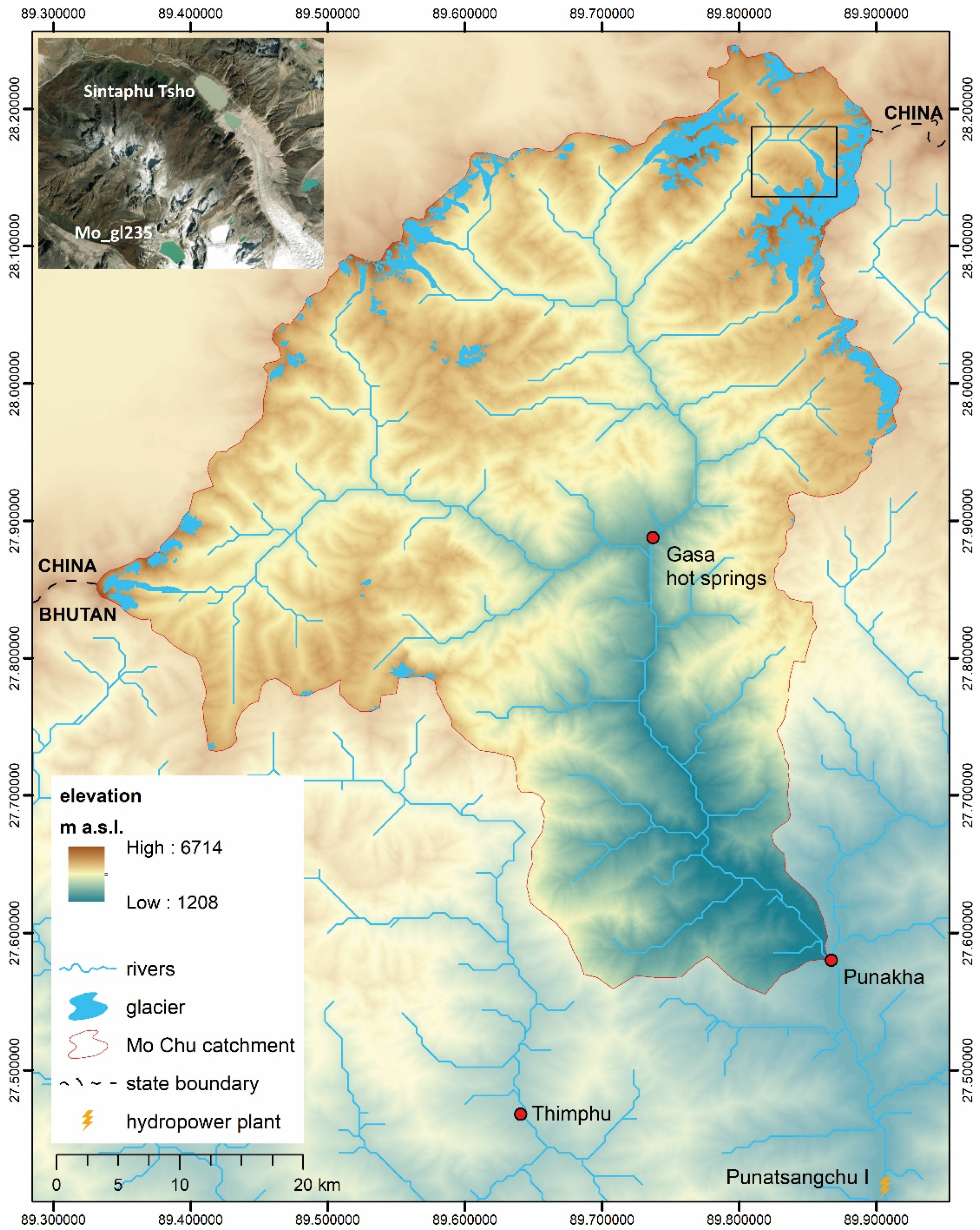
2. Study Site
3. Materials and Methods
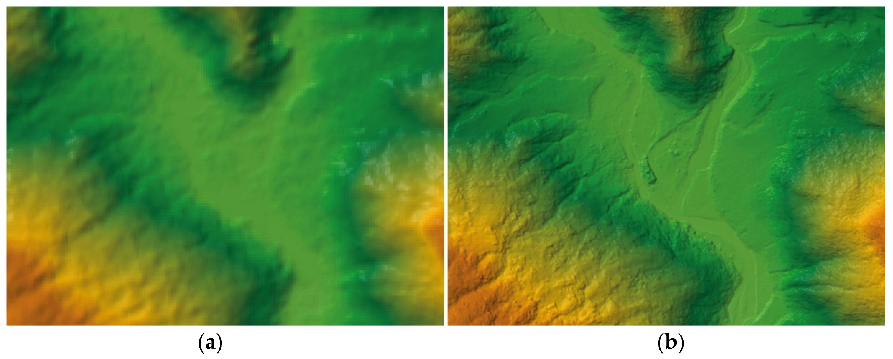
3.1. Digital Elevation Models
3.2. Hydrodynamic Modelling Using HEC-RAS 5.0.7
4. Results
4.1. GLOF Hydrographs
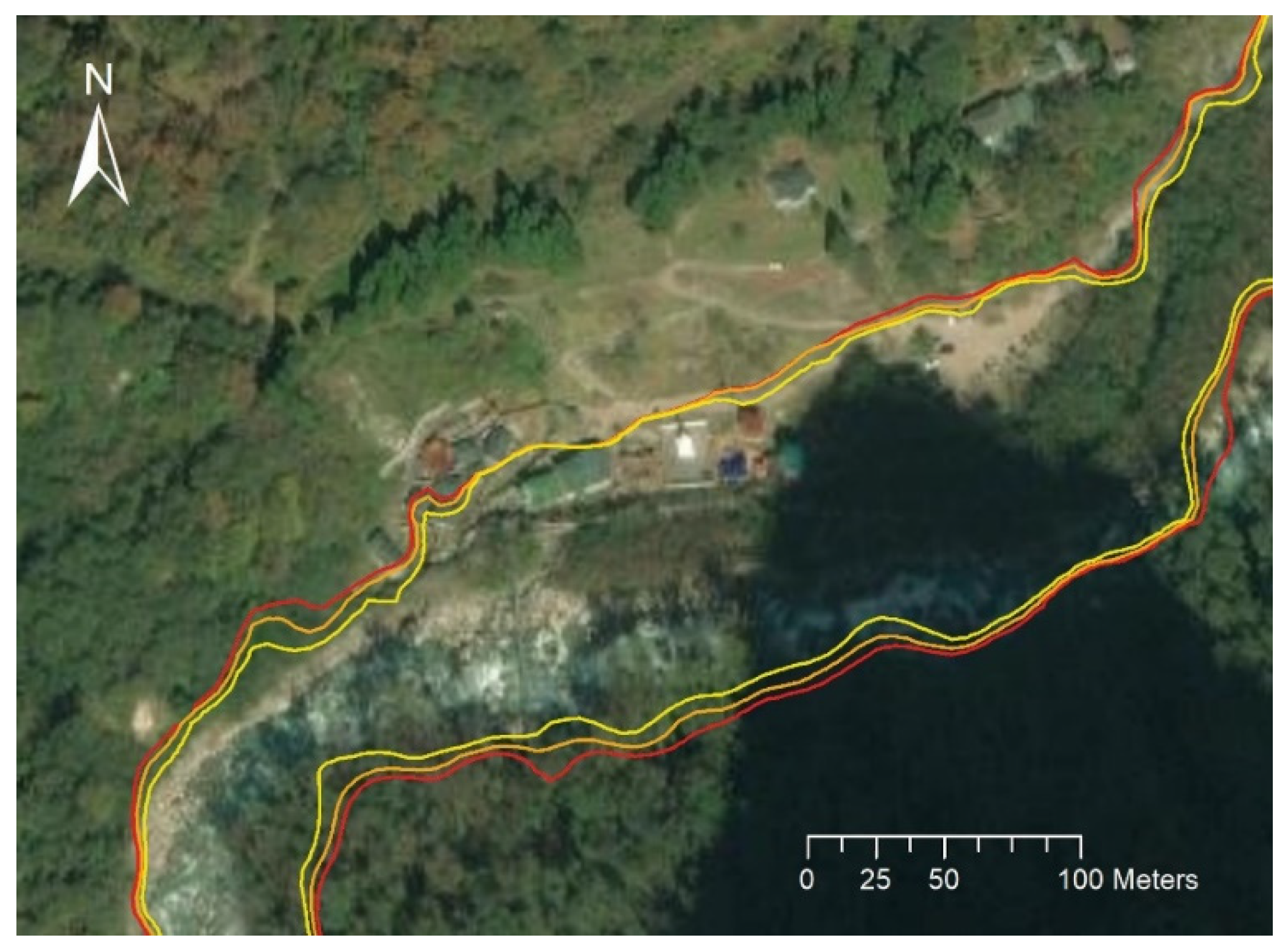
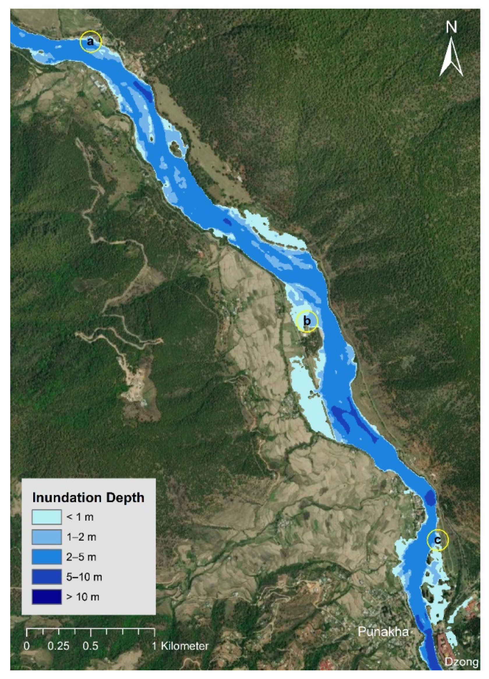
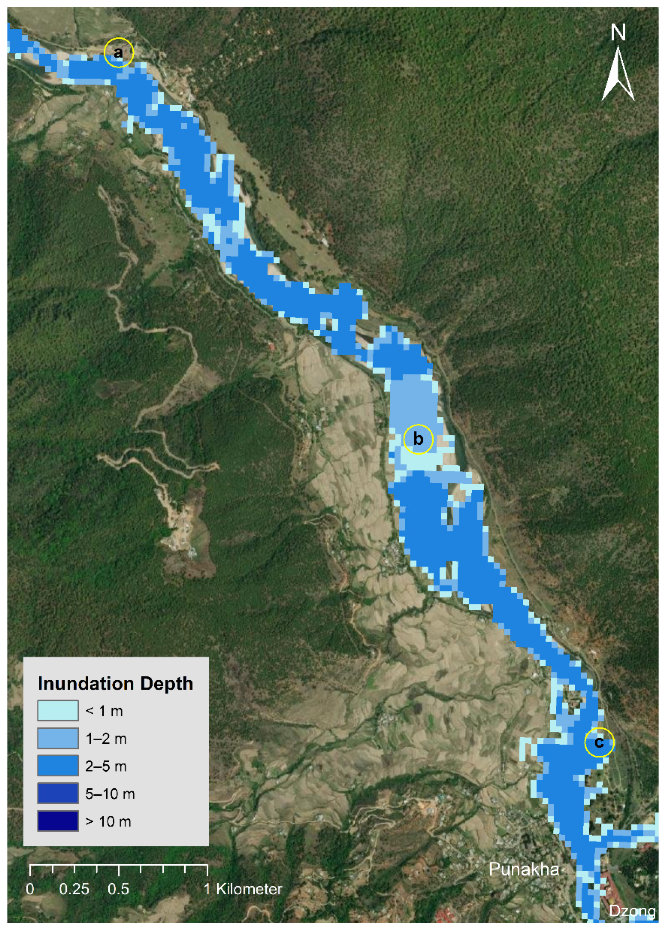
4.2. Timing and Inundation
4.3. Comparison with SRTM
4.4. Hazard Potential
5. Discussion and Conclusions
Author Contributions
Funding
Institutional Review Board Statement
Informed Consent Statement
Data Availability Statement
Acknowledgments
Conflicts of Interest
References
- Shugar, D.H.; Burr, A.; Haritashya, U.K.; Kargel, J.S.; Watson, C.S.; Kennedy, M.C.; Bevington, A.R.; Betts, R.A.; Harrison, S.; Strattman, K. Rapid worldwide growth of glacial lakes since 1990. Nat. Clim. Chang. 2020, 10, 939–945. [Google Scholar] [CrossRef]
- Clague, J.J.; Evans, S.G. A review of catastrophic drainage of moraine-dammed lakes in British Columbia. Quat. Sci. Rev. 2000, 19, 1763–1783. [Google Scholar] [CrossRef]
- Maharjan, S.B.; Mool, P.K.; Lizong, W.; Xiao, G.; Shrestha, F.; Shrestha, R.B.; Khanal, N.R. The Status of Glacial Lakes in the Hindu Kush Himalaya; ICIMOD Reserach Report 2018/1; ICIMOD: Kathmandu, Nepal, 2018. [Google Scholar]
- Gardelle, J.; Arnaud, Y.; Berthier, E. Contrasted evolution of glacial lakes along the Hindu Kush Himalaya mountain range between 1990 and 2009. Glob. Planet. Chang. 2011, 75, 47–55. [Google Scholar] [CrossRef] [Green Version]
- Komori, J.; Koike, T.; Yamanokuchi, T.; Tshering, P. Glacial lake outburst events in the Bhutan Himalayas. Glob. Environ. Res. 2012, 16, 59–70. [Google Scholar]
- Gurung, D.R.; Khanal, N.R.; Bajracharya, S.R.; Tsering, K.; Joshi, S.; Tshering, P.; Chhetri, L.K.; Lotay, Y.; Penjor, T. Lemthang Tsho glacial Lake outburst flood (GLOF) in Bhutan: Cause and impact. Geoenviron. Disasters 2017, 4, 17. [Google Scholar] [CrossRef] [Green Version]
- Watanbe, T.; Rothacher, D. The 1994 Lugge Tsho Glacial Lake Outburst Flood, Bhutan Himalaya. Mt. Res. Dev. 1996, 16, 77–81. [Google Scholar] [CrossRef]
- Richardson, S.D.; Reynolds, J.M. An overview of glacial hazards in the Himalayas. Quat. Int. 2000, 65–66, 31–47. [Google Scholar] [CrossRef]
- Huggel, C.; Haeberli, W.; Kääb, A.; Bieri, D.; Richardson, S. An assessment procedure for glacial hazards in the Swiss Alps. Can. Geotech. J. 2004, 41, 1068–1083. [Google Scholar] [CrossRef]
- Mool, P.; Wangda, D.; Bajracharya, S.R.; Kunzang, K.; Gurung, D.R.; Joshi, S.P. Inventory of Glaciers, Glacial Lakes, and Glacial Lake Outburst Floods: Monitoring and Early Warning Systems in the Hindu Kush-Himalayan Region, Bhutan; International Centre for Integrated Mountain Development (ICIMOD): Kathmandu, Nepal, 2001; ISBN 9291153451. [Google Scholar]
- Ukita, J.; Narama, C.; Tadono, T.; Yamanokuchi, T.; Tomiyama, N.; Kawamoto, S.; Abe, C.; Uda, T.; Yabuki, H.; Fujita, K.; et al. Glacial lake inventory of Bhutan using ALOS data: Methods and preliminary results. Ann. Glaciol. 2011, 52, 65–71. [Google Scholar] [CrossRef] [Green Version]
- Nagai, H.; Ukita, J.; Narama, C.; FUJITA, K.; Sakai, A.; Tadono, T.; Yamanokuchi, T.; Tomiyama, N. Evaluating the Scale and Potential of GLOF in the Bhutan Himalayas Using a Satellite-Based Integral Glacier-Glacial Lake Inventory Lake Inventory. Geosciences 2017, 7, 77. [Google Scholar] [CrossRef] [Green Version]
- NCHM. Reassessment of Potentially Dangerous Glacial Lakes in Bhutan; NCHM: Thimphu, Bhutan, 2019. [Google Scholar]
- Osti, R.; Egashira, S.; Adikari, Y. Prediction and assessment of multiple glacial lake outburst floods scenario in Pho Chu River basin, Bhutan. Hydrol. Process. 2013, 27, 262–274. [Google Scholar] [CrossRef]
- Petrakov, D.A.; Tutubalina, O.V.; Aleinikov, A.A. Monitoring of Bashkara Glacier Lakes (Central Caucasus, Russia) and Modelling of Their Potential Outburst; Springer: Dordrecht, The Netherlands, 2012. [Google Scholar]
- Worni, R.; Stoffel, M.; Huggel, C.; Volz, C.; Casteller, A.; Luckman, B. Analysis and dynamic modeling of a moraine failure and glacier lake outburst flood at Ventisquero Negro, Patagonian Andes (Argentina). J. Hydrol. 2012, 444–445, 134–145. [Google Scholar] [CrossRef]
- Byers, A.C.; Chand, M.B.; Lala, J.; Shrestha, M.; Byers, E.A.; Watanabe, T. Reconstructing the History of Glacial Lake Outburst Floods (GLOF) in the Kanchenjunga Conservation Area, East Nepal: An Interdisciplinary Approach. Sustainability 2020, 12, 5407. [Google Scholar] [CrossRef]
- Klimeš, J.; Benešová, M.; Vilímek, V.; Bouška, P.; Cochachin Rapre, A. The reconstruction of a glacial lake outburst flood using HEC-RAS and its significance for future hazard assessments: An example from Lake 513 in the Cordillera Blanca, Peru. Nat. Hazards 2014, 71, 1617–1638. [Google Scholar] [CrossRef]
- Karma, T.; Ageta, Y.; Naito, N.; Iwata, S.; Yabuki, H. Glacier distribution in the Himalayas and glacier shrinkage from 1963 to 1993 in the Bhutan Himalayas. Bull. Glaciol. Res. 2003, 20, 29–40. [Google Scholar]
- Bajracharya, S.R.; Maharjan, S.B.; Shrestha, F. The status and decadal change of glaciers in Bhutan from the 1980s to 2010 based on satellite data. Ann. Glaciol. 2014, 55, 159–166. [Google Scholar] [CrossRef] [Green Version]
- NCHM. Bhutan Glacial Lake Inventory (BGLI) 2021; NCHM: Thimphu, Bhutan, 2021. [Google Scholar]
- Anacona, P.I.; Mackintosh, A.; Norton, K. Reconstruction of a glacial lake outburst flood (GLOF) in the Engaño Valley, Chilean Patagonia: Lessons for GLOF risk management. Sci. Total Environ. 2015, 527–528, 1–11. [Google Scholar] [CrossRef] [PubMed]
- Sattar, A.; Goswami, A.; Kulkarni, A.V.; Emmer, A. Lake Evolution, Hydrodynamic Outburst Flood Modeling and Sensitivity Analysis in the Central Himalaya: A Case Study. Water 2020, 12, 237. [Google Scholar] [CrossRef] [Green Version]
- Uttenthaler, A.; Barner, F.; Hass, T.; Makiola, J.; D’Angelo, P.; Reinartz, P.; Carl, S.; Steiner, K. Euro-Maps 3D—A Transnational, High-Resolution Digital Surface Model for Europe, Edinburgh. 2013. Available online: https://www.euromap.de/pdf/euro-maps%203d%20-%20a%20transnational,%20high-resolution%20digital%20surface%20model%20for%20europe_anut_v1.0_20130911.pdf (accessed on 15 August 2021).
- Wang, W.; Gao, Y.; Iribarren Anacona, P.; Lei, Y.; Xiang, Y.; Zhang, G.; Li, S.; Lu, A. Integrated hazard assessment of Cirenmaco glacial lake in Zhangzangbo valley, Central Himalayas. Geomorphology 2018, 306, 292–305. [Google Scholar] [CrossRef]
- Kougkoulos, I.; Cook, S.J.; Edwards, L.A.; Clarke, L.J.; Symeonakis, E.; Dortch, J.M.; Nesbitt, K. Modelling glacial lake outburst flood impacts in the Bolivian Andes. Nat. Hazards 2018, 94, 1415–1438. [Google Scholar] [CrossRef] [Green Version]
- Brunner, G.W. HEC-RAS River Analysis System User’s Manual; US Army Corps of Engineers: Davis, CA, USA, 2016.
- Westoby, M.J.; Glasser, N.F.; Hambrey, M.J.; Brasington, J.; Reynolds, J.M.; Hassan, M.A.A.M. Reconstructing historic Glacial Lake Outburst Floods through numerical modelling and geomorphological assessment: Extreme events in the Himalaya. Earth Surf. Process. Landf. 2014, 39, 1675–1692. [Google Scholar] [CrossRef] [Green Version]
- Froehlich, D.C. Embankment Dam Breach Parameters and Their Uncertainties. J. Hydraul. Eng. 2008, 134, 1708–1721. [Google Scholar] [CrossRef]
- Arcement, G.J.; Schneider, V.R. Guide for Selecting Manning’s Roughness Coefficients for Natural Channels and Flood Plains; USGS: Denver, CO, USA, 1989.
- Kattelman, R.; Watanbe, T. Draining Himalayan Glacial Lakes before They Burst; IAHS Publication: Wallingford, UK, 1997; Volume 239, pp. 337–343. [Google Scholar]


| 90% Outburst | 70% Outburst | 40% Outburst | |
|---|---|---|---|
| Vw: outburst volume (106 m³) | 5.58 | 4.34 | 2.48 |
| Hb: breach depth (m) | 43 | 30.2 | 17.2 |
| tf: breach formation time (h) | 0.31 | 0.39 | 0.51 |
| B: mean breach width (m) | 45.3 | 41.2 | 33.7 |
| Scenario | Arrival Time Punakha (h:mm) | Arrival Time Punatsangchu I (h:mm) | Mean Max Velocity Dam-Punakha (m/s) | Inundation Area Dam-Punakha (km²) | Mean Flood Depth Dam-Punakha (m) |
|---|---|---|---|---|---|
| 90_0.04 | 3:54 | 6:10 | 5.6 | 13.38 | 5.72 |
| 90_0.06 | 4:30 | 7:50 | 4.7 | 13.57 | 5.79 |
| 90_0.08 | 5:12 | 8:46 | 4 | 13.65 | 5.88 |
| 70_0.04 | 4:16 | 6:50 | 5 | 12.35 | 4.69 |
| 70_0.06 | 5:00 | 8:36 | 4.1 | 12.49 | 4.79 |
| 70_0.08 | 5:46 | 9:48 | 3.5 | 12.63 | 4.90 |
| 40_0.04 | 5:06 | 8:12 | 3.9 | 10.56 | 3.35 |
| 40_0.06 | 6:04 | 10:24 | 3.1 | 10.77 | 3.44 |
| 40_0.08 | 7:00 | 12:50 | 2.6 | 10.97 | 3.53 |
Publisher’s Note: MDPI stays neutral with regard to jurisdictional claims in published maps and institutional affiliations. |
© 2021 by the authors. Licensee MDPI, Basel, Switzerland. This article is an open access article distributed under the terms and conditions of the Creative Commons Attribution (CC BY) license (https://creativecommons.org/licenses/by/4.0/).
Share and Cite
Hagg, W.; Ram, S.; Klaus, A.; Aschauer, S.; Babernits, S.; Brand, D.; Guggemoos, P.; Pappas, T. Hazard Assessment for a Glacier Lake Outburst Flood in the Mo Chu River Basin, Bhutan. Appl. Sci. 2021, 11, 9463. https://doi.org/10.3390/app11209463
Hagg W, Ram S, Klaus A, Aschauer S, Babernits S, Brand D, Guggemoos P, Pappas T. Hazard Assessment for a Glacier Lake Outburst Flood in the Mo Chu River Basin, Bhutan. Applied Sciences. 2021; 11(20):9463. https://doi.org/10.3390/app11209463
Chicago/Turabian StyleHagg, Wilfried, Stefan Ram, Alexander Klaus, Simon Aschauer, Sinan Babernits, Dennis Brand, Peter Guggemoos, and Theodor Pappas. 2021. "Hazard Assessment for a Glacier Lake Outburst Flood in the Mo Chu River Basin, Bhutan" Applied Sciences 11, no. 20: 9463. https://doi.org/10.3390/app11209463