Abstract
Recently, food recognition has received more research attention for mHealth applications that use automated visual-based methods to assess dietary intake. The goal is to improve the food diaries by addressing the challenges faced by existing methodologies. In addition to the classical challenge of the absence of rigid food structure and intra-class variations, food diaries employing deep networks trained with pristine images are susceptible to quality variations in real-world conditions of image acquisition and transmission. Similarly, existing progressive classifiers that use visual features via a convolutional neural network (CNN) classify food categories and cannot detect food ingredients. We aim to provide a system that selects the optimal subset of features from quality resilient CNNs and subsequently incorporates the parallel type of classification to tackle such challenges. The first progressive classifier recognizes food categories, and its multilabel extension detects food ingredients. Following this idea, after extracting features from the quality resilient category and ingredient CNN models by fine-tuning it on synthetic images generated using the novel online data augmentation method random iterative mixup. Our feature selection strategy uses the Shapley additive explanation (SHAP) values from the gradient explainer to select the best features. Then, novel progressive kernel extreme learning machine (PKELM) is exploited to cater to domain variations due to quality distortions, intra-class variations, and so forth, by remodeling the network structure based on activity value with the nodes. PKELM extension for multilabel classification detects ingredients by employing a bipolar step function to process test output and then selecting the column labels of the resulting matrix with a value of one. Moreover, during online learning, the PKELM novelty detection mechanism can label unlabeled instances and detect noisy samples. Experimental results showed superior performance on an integrated set of measures for seven publicly available food datasets.
1. Introduction
Progressive learning is the natural continuous learning process exhibited by humans. There is no limit to the training and testing process, and whenever the human brain is tripped against new concepts, learning resumes. This learning process creates new neurons and remodels existing neurons in the brain. The formation of new neurons decreases the plasticity of the old neurons. The key feature of the human learning process is that the acquisition of new concepts or domain variations does not affect the existing knowledge.
These aspects of progressive learning demonstrate their importance in many real-world recognition problems, including food recognition. Food datasets have high diversity due to the continuous arrival of new food categories and ingredients. The definitions of the concepts are different for each person due to several cooking procedures to prepare the same food type. Similarly, in practical computer vision applications, an input image undergoes some form of distortion that causes domain variations. These attributes of food datasets require a network that can mimic the properties of progressive learning as exhibited by humans. The proposed network should remodel automatically by adding new nodes, parameters and interconnections for the novel task while reducing catastrophic forgetting and negative forward and backward transfer for previous concepts.
Although in the recent era, food recognition by computer vision methods has attained much attention among the research community, in practical applications, multiple challenges associated with modern techniques have increased the gap with the laboratory environment. In practical food recognition applications, the food photo taken from the mobile camera varies in quality. These variations in picture quality make features extracted from the deep model susceptible to quality distortions. Secondly, the fully connected classifier in deep learning models and other batch classifiers has a fixed class architecture and is unsuitable for progressive learning. Incremental classifiers for food recognition partially address this problem by using features from the deep model due to its good generalization ability [1]. However, high dimensions of deep features increase training time and computational complexity. Previous studies use classical techniques such as ReliefF and so forth [2] to reduce the feature dimension. These feature selection methods have black box behavior, and there are no visual explanations of selected features. Finally, most of the existing literature and the incremental classifier proposed by Ghalib et al. [1] classify only food categories and do not classify food ingredients. The classification of food ingredients has pivotal importance for dietary assessment apps. By keeping in view these challenges, this work makes several contributions to the food recognition literature.
(1) This work provides an evaluation of the InceptionResNetV2 model employed for feature extraction under quality distortions. It considers five common types of distortions: Gaussian blur, defocus blur, Gaussian noise, JPEG, contrast. Based on the evaluation, we extracted feature vectors from the quality resilient InceptionResNetV2 model after fine-tuning it on synthetic images generated using our novel data augmentation method “random iterative mixup” at no extra training cost. To the best of our knowledge, it is the first detailed evaluation available for food datasets and the first method to tackle quality distortions in the images for food datasets;
(2) We analyzed the visualizations from the Gradient Explainer, which shows that all the pixels in an area of interest do not contribute equally or positively to the desired output. Based on our findings, we introduced a feature selection technique that uses SHAP scores from the gradient explainer to select the optimal subset of features from the high dimension space by filtering out the irrelevant ones;
(3) We introduced PKELM for food categorization and ingredient recognition. It uses the activation value for creating and updating the mapping nodes and successfully replaces the random selection in adaptive reduced class incremental kernel extreme learning machine (ARCIKELM). Its progression strategy caters to domain variations while reducing the computational complexity of the kernel matrix during online learning by growing when required. Moreover, during online learning, the novelty detection mechanism of PKELM detects label noise and assigns labels to those unlabeled training instances.
2. Related Work
We examine the existing methodologies that have been developed so far for automatic food recognition. It includes approaches ranging from distance-based methods, a probabilistic model and decision tree, support vector machine, extreme learning machine, convolution neural networks to ensembles.
Herranz et al. studied the probabilistic model and decision tree for the food, restaurant, and dish images dataset [3]. Several approaches use distance-based methodology for food image classification [4,5]. These classifiers used handcrafted features such as color and wavelet texture properties, Gabor, Shape, scale-invariant feature transform (SIFT), and Bag of Features (BoF) for learning. The handcrafted features from these methods are not robust to image quality. Moreover, these classifiers do not incrementally learn new food concepts and ingredients.
Support vector machine is widely applied to classify features extracted from different methods. Yoshiyuki et al. [6] used a fisher vector for encoding histogram of oriented gradients (HOG) and color patches. Some variants of support vector machine (SVM) uses features from a bag of words, color histogram, and the D-SIFT approach [7]. The researchers also explored local, including global and color, features [8], SIFT and Shape context descriptors [9], and pairwise local features [10] for training SVM. Several SVM methods use the edge detection method [11], counting the pixels in the region of interest, SIFT-BoF, Color-Sift with the spatial pyramid [12], Color hue, and multiple types of SIFT features [13]. Some research work focuses on the hybrid aggregation of sparse, color, and edge histogram [14] for feature extraction and SVM for classification. The multi-view multi-kernel SVM [15] detects both ingredients and categories, but it has high computational complexity, and it cannot learn novel concepts. Several food logging applications integrate the SVM-based frameworks [6,16]. However, most of these studies focused on the feature extraction part. They have used fixed-class architecture for classification, which does not progressively learn new food classes and ingredients. Moreover, they have not employed explainable artificial intelligence (AI) methods to understand the contributions of an area of interest in the food photos towards model predictions.
Convolutional neural networks have achieved state-of-the-art performances on many food recognition datasets [17,18,19,20,21]. Recent studies have explored a variety of CNN-based methods for their datasets. These methods range from the asymmetric multi-task convolutional neural network [22] and the spatial pyramid convolutional neural network [22] to the multi-scale multi-view deep network [23]. However, none of these methods studied the impact of quality distortion in the images on the robustness of features. These studies used a linear-fully connected classifier of CNN for classification, which has a fixed structure. It cannot progressively learn new food classes and ingredients. It is noteworthy that most studies classify only food categories. Jing et al. [24] proposed Arch-D architecture for detecting food categories and ingredients. However, their method uses batch learning and, as a result, it cannot adapt domain changes within the existing concepts or learn new classes. Sequential personalized classifier (SPC) [25] is a personalized framework for food recognition that only classifies food categorizes. During online learning, SPC is unable to detect data instances with noisy labels. SPC also does not assign labels to an unlabeled dataset. Moreover, it does not interpret the contribution of the pixels in food photos towards classification.
Recently, researchers scrutinized extreme learning machines for food classification. Supervised Extreme Learning Committee [26], uses committee members, “kernel extreme learning machine” trained to specialize single feature type. It has high complexity as it uses all the features of training images for computing kernel matrix. Ghalib et al. [1] recently proposed ARCIKELM for open-ended learning. The classifier randomly selects 10 percent of data points as mapping nodes for computing the kernel matrix. Moreover, they have only studied the classification of food categories.
In summary, comprehensive literature shows several research gaps in existing methods and frameworks. Many existing studies, which employed classical methods for food classification, focus only on feature engineering. With the rise of deep learning, recent methods use CNN features due to their good generalization ability. However, quality distortions, such as blur and Gaussian noise in the images that occur during image acquisition, reduce the robustness of these features. Following that, selecting the optimal features from the deep model is a challenge due to many domain-specific problems in food recognition, such as non-rigid structure and intraclass variations. Then, for classification, many methods employed have a fixed-class architecture. They cannot tackle domain variations due to changes in concepts or quality distortions and so forth, and they can detect either food categories or ingredients.
Based on these research gaps, the proposed framework contributes to the existing literature by evaluating the impact of quality distortions in the images on the features from the deep model. It then uses a novel data augmentation strategy, RIMixUp, during fine-tuning to improve the robustness of the model. As a result, feature vectors extracted are more invariant to distortions in the food images. Following that, it selects optimal subsets of features by using a strategy based on Gradient Explainer. Then the article employs a novel PKELM classifier to progressively learn from optimal feature vectors and tackle domain variations during online learning.
3. Methodology
3.1. General Architecture
The pipeline of our framework extracts quality resilient features from category CNN and the ingredient CNN model. The method selects the best features by using the SHAP values from the gradient explainer by filtering out the irrelevant ones. Then, it uses a novel progressive kernel extreme learning machine (PKELM) and its multilabel extension for food category and ingredient classification. Figure 1 shows the architecture diagram. During the training phase, category CNN and ingredient CNN, using the InceptionResNetV2 model as a backbone structure, extract feature vectors from training images. After feature extraction, it selects reliable feature vectors using a feature selection strategy based on Gradient Explainer. The novel PKELM classifier and its extension for multilabel classification progressively learn from the optimal feature vectors of the images to detect food categories and ingredients.
During the classification of the test image, the first step is to extract the feature vectors from the fully connected layer of the category and ingredient CNN. The extracted feature vectors from the category network and the ingredient network have a dimension of 1536 and 1024. After that, the feature selection process selects the 500 most relevant attributes from each feature vector. Finally, PKELM classifies food categories and ingredients by using the optimal feature vectors.

Figure 1.
Flow chart of the proposed framework. The red dot presents new neurons during progressive learning.
Figure 1.
Flow chart of the proposed framework. The red dot presents new neurons during progressive learning.

3.2. Visual Features via Quality Resilient Convolutional Neural Network
Visual features extracted from the food photos with various quality distortions via a quality resilient convolutional neural network (CNN) are nearly as discriminatory as the features from the pristine images. In an ideal case, the visual feature vectors from the pristine and distorted food photos must be equally discriminant with similar classification accuracy.
Previous research by Ghalib et al. [1] found that for food category datasets, features extracted from the fine-tuned InceptionResNetV2 model have superior classification performance as compared to ResNet-50 and DenseNet-201 model. Based on their findings, we employed the InceptionResNetV2 model pre-trained on the ImageNet dataset and fine-tuned it on food datasets for feature extraction. However, in real-world settings, the poor quality of food photos affects the robustness of the model employed for feature extraction. An evaluation is provided of the InceptionResNetV2 to study the impact on the model under five common types of image distortions: (1) Gaussian blur; (2) Gaussian noise; (3) Defocus blur; (4) Contrast; (5) JPEG Compression [27] that occurs in the real-world situation at different parameter settings. Then, to improve the robustness of the model for the most expected distortions in practical applications, we fine-tuned the network employed for feature extraction on food images using our novel data augmentation strategy RIMixUp. The idea behind our data augmentation method is to generate a single synthetic image that carries the knowledge of clean and noisy images. Based on this idea, proposed data augmentation advances the mixup theory to generate a single synthetic image for tackling quality distortions. We exploited mixup theory, as theoretical analysis by Zhang et al. [28] shows that mixup regularizes the neural network to favor simple linear behavior in-between training examples. As a result, it improves generalization and robustness. Figure 2 gives a visual illustration of our process. In step1, it generates a single image by iteratively mixing randomly selected images distorted with Gaussian noise, defocus blur, and Gaussian blur using the mixup strategy [29]. The method generates a new synthetic image by mixing the pristine image with the synthetic image generated in step 1, using the mixup strategy. Equations (1) and (2) generates the synthetic images.
where are the raw input vectors of the clean images and are the random iterative mixup of raw input vectors of the noisy images. Similarly, are the one-hot label encodings of clean images, and are the random iterative mixup of one hot label encodings. Here are values with [0, 1] range and are sampled from the beta distribution. (, ) refers to the final synthetic training samples. Synthetic images generated using RIMixup data augmentation for the food datasets fine-tunes the InceptionResnetV2 model pre-loaded with weights trained on ImageNet. Figure 3 shows the process of training a quality resilient convolutional neural network (CNN) to extract visual features. Our approach makes the model used for feature extraction more invariant to image quality. It has several benefits in contrast to state-of-the-art methods for the most expected distortions levels. Unlike DeepCorrect [30], it does not require any change in the architecture of the model. It does not increase training time like fine-tuning with low-quality images, as the size of the training data remains the same. Nor does it increase the number of FLOPS for the test image. Unlike stability, training [31] and feature quantization methods [32], it does not affect the top 1 accuracy of the pristine images. In the experimental section of this work, we have briefly discussed our findings.
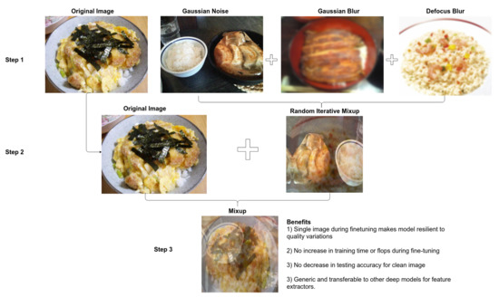
Figure 2.
Proposed data augmentation for quality resilient feature extraction.
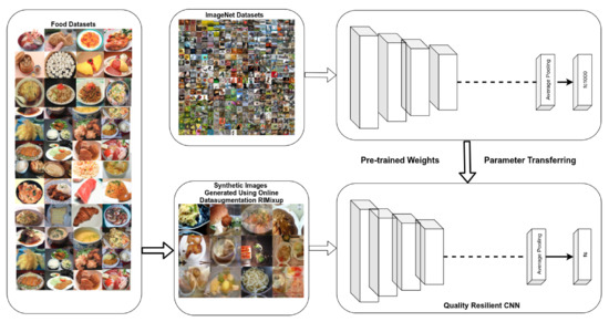
Figure 3.
Quality resilient convolutional neural network (CNN) to extract visual features.
3.3. Gradient/Deep Explainer Based Strategy for Feature Selection
We employed a strategy that uses SHAP values [33] from Shapley Additive exPlanation methods: (1) Gradient Explainer; and (2) Deep Explainer to rank and filter the irrelevant features. The Gradient Explainer combines the ideas from Integrated Gradients, SHAP, and Smooth Grad into a single expected equation. It approximates the model as a linear function between each background data sample and input feature vector. The attributes are assumed to be independent of each other and then expected gradients compute approximate SHAP values.
Similarly, Deep Explainer builds a connection with Deep Lift to calculate the SHAP values of a deep learning model. It computes SHAP values by assuming that input attributes are independent of one another. The deep model is linear, and this approach combines SHAP values of smaller components of the network into the whole network’s SHAP values. Equation (3) computes the linear approximation.
SHAP values of both techniques integrate the conditional expectations with game theory and classic Shapley values to assign the values to the attributes of the feature vector. Their explanation model e satisfies the three properties of (1) Local accuracy; (2) Missingness; and (3) Consistency, as shown in Equation (4).
Here, , S represents the set of non-zero indexes in where . is the expected value of the function conditioned on a subset S of the input features, M indicates the number of features and N refers to the set of all input features.
Feature Selection Steps for High-Dimensional Class-Imbalanced Image Data
The proposed algorithm uses the SHAP score values from the Gradient Explainer and Deep Explainer to measure the importance of each attribute for the output layer. For food category and ingredient detection, we compute the SHAP values of each food image in the training dataset from the max-pooling layer (8, 8, 1536) of the InceptionResNetV2 model. The ranked output parameter value is 1 for all food category datasets. As there are multiple labels in multilabel classification for ingredients detection, the ranked output parameter value is the average number of ingredients in the dataset. After that, we applied average pooling to obtain a single vector (1, 1536) of each image for food category datasets. In the case of food ingredient datasets after average pooling, we will get vectors equal to the ranked outputs, so we took the average of these vectors to get the single vector. The SHAP score of each food class c is the average SHAP scores of the training instances belonging to that class. Equation (5) represents the mathematical form to compute the SHAP score of each food class.
where refers to the SHAP score vector of ith training instance and t refers to the total images in the class. Then, we computed the SHAP score of each attribute as in Equation (6) by taking the mean of each class SHAP score vector.
Here, refers to the SHAP score vector of the ith food class, and c refers to the total number of food classes. Following that, the feature selector ranks the attributes and selects the 500 attributes with the highest score. Algorithm 1 shows steps of the feature selection method. Figure 4 diagrammatically illustrates the process of feature selection. In the results section, the article presented the results of the performance comparison of the proposed feature selection strategy with a classical ReliefF method for all the food datasets.


Figure 4.
Shows the process of the feature selection.
Figure 4.
Shows the process of the feature selection.
| Algorithm 1 Feature selection steps based on Gradient/Deep explainer |
| Input - Feature vectors of training/test images extracted from the fully connected layer of the InceptionResNetV2 model. - Training images - Ranked outputs Output Indexes of selected attributes. Algorithm 1. Load deep learning model (InceptionResNetV2). 2. for i = 1 to c 3. for k = 1 to t 4. For the input image, compute the SHAP score of the attributes at the max pooling layer using gradient explainer according to Equation (4). 5. Apply average pooling to get a single vector of SHAP values. In case, the ranked outputs are more than 1 take average to get single vector. 6. Add the feature vector of SHAP values with the sum of SHAP values of previous feature vectors. 7. endfor 8. Compute the average SHAP score of each attribute of the feature vectors for the class by using Equation (5). 9. endfor 10. Compute the mean score of each attribute by taking the average SHAP score of all classes using Equation (6). 11. Determine the indexes of attributes with the highest SHAP score. 12. Select the features from training/testing feature vectors corresponding to indexes y of attributes with the highest SHAP score. |
3.4. Progressive Learning for Food Category and Ingredient Classification
This section presents a novel classifier for progressively learning food categories and ingredients from optimal feature vectors. The article hypothesizes that randomly selecting mapping nodes from the training dataset does not ever best represent the food classes, especially during online learning. However, the growing when required (GWR) dynamically creates and updates mapping nodes when the current state of the network does not sufficiently match the input. This strategy tackles domain variations in existing classes and learns novel concepts by decreasing plasticity on old neurons. For this reason, it has employed the mechanism of GWR for creating and updating mapping nodes [34] during progressive learning in the PKELM classifier. It also optimizes the kernel matrix by selecting only relevant support vectors instead of using all data points for computing the kernel matrix. The following subsection discusses the background of our work, followed by the detailed working of our model.
3.4.1. Adaptive Reduced Class Incremental Kernel Extreme Learning Machine
The adaptive reduce class incremental kernel extreme learning machine is proposed by Ghalib et al. [1]. The method incrementally learns new classes and adjusts hidden neurons to reduce plasticity on old neurons, making the classifier suitable for continual food recognition. This section has explained its mathematical working.
Initialization Phase
In the initialization phase, 10 percent of data from the base classes are used as mapping nodes to train the algorithm, like reduce kernel extreme learning machine. Following that, it initializes the dynamic “Neuron Eligibility” matrix. The matrix contains the activation information of each neuron.
Adding New Class
When novel class arrives, it selects the 10 percent of data of the new class and updates the output weights by multiplying them with the transformation matrix. The method increases the total number of output neurons in the network by one. The network inserts the nodes from the novel classes into the kernel matrix by using “growing neuron methodology” [1]. Corresponding to that, they update the “Neuron Activation” matrix, and its size will become equal to the total number of neurons in the kernel matrix.
Growing Hidden Neurons
Ghalib et al. [1] enhanced a methodology of Constructive Enhancement OS-ELM for incrementally inserting the hidden neurons in ARCIKELM. They have used the kernel matrix to compute the weights for new nodes instead of randomly choosing the input weights.
From the existing knowledge [1] when it inserts new hidden neurons into the network. The hidden layer output matrix will expand as it adds more columns into K. Now consider the new chunk of data arrives, and there is a need to add new hidden neurons, then the method uses Equations (7) and (11) to expand the hidden layer output matrix.
where,
Sequential Learning
During sequential learning, when data of the existing class arrives it checks the similarity by using the multidimensional Gaussian function. When the incoming data vector is close to neurons in the kernel matrix, the membership degree is high, and the method sequentially updates the network as new hidden neurons are not required. If it is away, then the membership degree is low. The neurons are added to the network when the max fuzzy membership value is less than the threshold. The threshold value is the user-defined parameter.
3.4.2. Progressive Kernel Extreme Learning Machine
When PKELM process an input feature vector, it computes the activity of each node in the map space and picks the winner node. If the best matching node has activity close to one, then the first winner represents the input node well. Thereon, PKELM trains the node and its neighbors. Following that, it decreases the counter and sequentially updates the kernel matrix and output weights. In the scenario, when the activity value is less than the threshold. Then, there is a mismatch between the node and input. If the node is the new one, it decreases the firing counter. Otherwise, the network inserts the new node to represent the input well and expands the corresponding kernel matrix using the “Growing Hidden Neuron” methodology. In addition, previous progressive classifiers are evaluated for food categorization, and they have not extended their methods for food ingredient detection. We extended PKELM for multilabel classification by using the bipolar strategy with a trivial threshold of 0. Despite the simplicity of our extension for multilabel classification, experiment analysis shows the superiority of this approach over the state-of-the-art methods while progressively learning new groups of ingredients. Table 1 presents the algorithm and Figure 5 shows architecture of PKELM classifier. We briefly discuss the mathematical working of the model as follows.

Table 1.
Proposed PKELM for food categorization and ingredient detection.
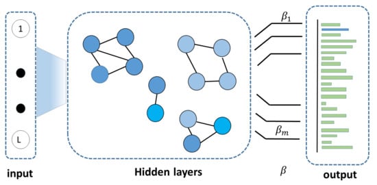
Figure 5.
Shows the architecture of PKELM classifier.
Let A denotes the set of map nodes. The is the set of connections of the nodes in the map field. The input distribution is denoted by for inputs. Define as the weight vector of node n.
Initialization Phase
In this phase, PKELM initializes the network by creating two mapping nodes . The nodes and are initialized randomly from the input distribution of the classes in the base session. The connection set C is set to empty . Following that, it computes the kernel matrix and output weights using the initial mapping nodes. Equation (12) computes the kernel matrix:
where is the initial kernel matrix, is the observed sample from base classes, and denotes the and mapping nodes. Equation (13) computes the initial output weights.
where,
There are two ways in the literature to encode label vectors : the first way encodes the label vectors as 0 or 1, and the second way encodes label vectors as or 1. This work encoded the label vectors as and 1. Encoding the label vectors as and 1 is necessary for our approach concerning multilabel classification, as PKELM employed the trivial threshold of 0 in a bipolar step function to select the labels.
Progressive Learning
After initialization, the proposed classifier incrementally learns new food categories and ingredients. The PKELM inserts new mapping nodes at any time and adjusts the structure. The new node is inserted into the network when the activation value of the best matching node is less than the threshold. The activation value is the Euclidean distance between the input representation of the food image and the weights of the nodes in the network.
Each iteration of the algorithm is as follows: For every node i of the network, the method computes the distance from input by using Equation (15).
where represents the input vector and refers to the weight of the ith mapping node.
The network selects the first best f and second best mapping node s based on Euclidean distance as in Equation (16).
where and represents the weight vector of the node n. If there is no connection between the first and second-best matching nodes, then create a new connection.
Compute the activity value with the best matching node as in Equation (18).
Here, refers to the incoming feature vector, and refers to the weight of the best matching node.
The age is set to zero when the link exists between the first best and second best. When the input feature vector belongs to a new food category or contains novel ingredients, then Equation (19) increases the output neurons in the network by multiplying the output weights with the transformation matrix. For food ingredient detection, the newly added output neurons will be equal to the total number of novel ingredients. All the columns corresponding to new neurons in the transformation matrix are set to zero.
where, M is a transformation matrix as in Equation (20),
Following that, if the activity is less than the activation threshold and the firing counter is less than the firing threshold, a new node m is inserted in the model between the winning node (badly matched) and the input. The weight vector of the newly added input node is initialized to the mean average of the weight of the input node and the best matching node.
Equation (22) computes the weight vector of the new mapping node , which is the average weight vector of the best matching node and the input node, and Equation (23) creates new edges, and Equation (24) removes link between first winner and second winner.
As the model adds a new mapping node, the “Growing Hidden Neuron Methodology” will update the kernel matrix by Equations (7)–(11). The and in Equations (7)–(11) is computed by Equations (25) and (26).
In the second scenario, when the best matching nodes represent the input well, the network will update the position of its winning node as in Equation (27), and its i neighbors by using Equation (28).
where , represents the value of firing counter of node f and then the age of the edges of the “first best match” neighbors is incremented by 1.
Here, refers to the age of the ith edge of the first best matched node with its neighbour.
After that, it computes the kernel matrix of chunk of data using Equation (30). Then it updates the network sequentially by using Equation (31).
where denotes the weights of all the nodes of the network.
Then, Equation (32) updates the output neurons.
Next, the firing frequency of the winning node f and its neighbors is reduced using the Equations (33) and (34). As frequently fired nodes are trained less, this sheds the problem that progressive network suffers from the weights of well-trained nodes and moves slightly.
Here, refers to the size of the firing variable of node i. refers to the initial strength and refers to stimulus strength which is usually 1. , , and are constants controlling the behavior of the curve. The network removes mapping nodes without edges or age higher than a certain threshold from the kernel matrix and network. This is a vital step in progressive learning as it continuously optimizes the network by removing irrelevant neurons from the model. When the new input data arrives, PKELM repeats the process, otherwise stopping criteria have been reached.
Testing Phase
During testing of incoming food representations, Equation (35) computes the kernel matrix between the incoming vector and weight vectors in the network. Thereon, Equation (36) computes the output Y vector.
The food category corresponding to the index of the highest value in the Y vector is selected. However, for ingredient detection, the input food representation contains multiple ingredients (Labels). PKELM used a bipolar step function with a trivial threshold t of “0” for detecting ingredients labels, corresponding to column Y. The values of Y are passed as an argument to the function as in Equation (37). The set of columns with values greater than zero gives the multi-label belongingness of the corresponding input.
where is the ith value of output vector Y and t refers to the threshold value.
It is to be noted that various kernels from the existing research work satisfy mercer’s condition. This research work has used the RBF kernel [35] and chi-square kernel [36]. The mathematical form of these kernel functions are as follows:
(1) RBF Kernel
(2) Chi-square Kernel
The experiment section briefly discusses the results of the comparison of PKELM with its predecessors.
Novelty/Noise Detection
During online learning, the expert should verify food images from users before updating the model to ensure data integrity. When a model is updated during online learning without verification of the food images, then noisy food images from mobile devices during online learning negatively affect the classification performance of the trained model. As the integrity of the data used to train the model is essential in a health care setting. However, manually validating each food image from the user before updating the classifier is a time-consuming process. So, it is necessary to automatically attenuate the noisy images and detect food images with novel concepts or domain variations in online food recognition. To semi-automate this, our proposed PKELM uses the activation function of the trained model. The activation response decreases exponentially for a higher distance between input and nodes in a network. When the response of the incoming input from the user is less than the threshold, the incoming input is labeled as a novel concept or domain variation not well represented by the existing nodes in the model. The threshold value is selected based on the response distribution of the training set. For every novel input, the incrementally trained PKELM computes by using Equation (40). In it, and represent the mean and standard deviation of activations on the food training dataset. is a constant value that modulates the influence of fluctuations in activity distribution.
when the value is less than the threshold, it is a novel concept or noise. The novelty detection mechanism in PKELM also assigns labels to unlabeled food representations whose response is greater than the threshold. Automatic labeling of unlabeled images helps to reduce the time cost required for manual labeling. The experimental section explains the results for detecting noisy non-food images and correctly assigning labels to the unlabeled data samples.
4. Experiment and Results
This section discusses the food datasets used for experimentation, implementation details of the proposed framework, and a detailed analysis of each method used in this study. There are three major components of the proposed framework: (1) Visual features Via Quality Resilient Convolutional Neural Network. The framework has used InceptionResNetV2 due to its superior performance over InceptionV3, Resnet 50 [1]. However, in a real-world scenario, images from mobile devices have varying quality levels. This paper investigated the InceptionResNetV2 model under different quality distortions. Then, it has tackled quality distortions by employing a novel data augmentation strategy random iterative mixup to fine tune quality resilient CNN for feature extraction; (2) Gradient/Deep Explainer Based Strategy for Feature Selection. The proposed algorithm has incorporated SHAP values from the Gradient Explainer [33] for reliable feature selection. This section briefly discusses the experimental results; (3) During the classification phase, the novel progressive learning method PKELM categorizes food (Multi-Class) and detects food ingredients (Multi-Label). Unlike existing works, it incrementally learns new food categories and ingredients from optimal feature vectors and adapts domain changes within existing concepts. This section briefly discusses the results of the food datasets.
4.1. Datasets
To evaluate the proposed framework, we used six food datasets extensively used by researchers previously. This section briefly describes the important features of the datasets. Table 2 shows attributes of food datasets for food category classification. Table 3 shows attributes of food datasets for ingredient detection. Figure 6 shows the complexity and variation of each food dataset.
4.1.1. Food101
The dataset consists of 101,000 food images which are categorized into 101 classes [37]. The dataset has many semantically similar images, which poses a challenge to the classifier. The extended versions “Ingredient101” of Food101 [38] has 446 unique food ingredients for multi-label classification with an average of 9 ingredients per recipe. We used the extended version to evaluate PKELM for ingredient detection.
4.1.2. UECFOOD100
This dataset contains 100 different types of food. Most of the foods included in this data set are famous food in Japan [12]. Some of these categories are also commonly known food in other parts of the world.
4.1.3. UECFOOD256
The dataset has the highest number of classes compared to other datasets used for evaluation purposes in this study. It is an extension of the UECFOOD100 dataset, and most of the food classes have Japanese foods [39]. Figure 6C shows the complexity and variations within the UECFOOD256 dataset.
4.1.4. Pakistani Food
It consists of 100 food classes of Pakistani Food Datasets, and it has 4928 food images [1]. It poses a challenge for progressive classifiers due to the complex variety of food dishes.
4.1.5. PFID-Baseline/PFID
PFID-baseline has 1388 food images categorized into 61 classes. In another combination of the PFID dataset, we have categorized it into 15 different types of groups. It is gathered from various chains and includes food such as pizza, salad, and burgers. It has three kinds of instances, and each of the data instances in the restaurant has images with the wrapper and four images without a wrapper [40]. Figure 6E shows inter-class similarity and intra-class dissimilarity of the PFID dataset.
4.1.6. VireoFood-172
The VireoFood-172 dataset contains 110,241 food images of 172 food categories of Chinese food dishes containing 353 ingredients. It has popular food categories from “Go cooking” and “Meishijie” [24].
Table 2.
Attributes of food datasets for food category classification.
Table 2.
Attributes of food datasets for food category classification.
| Dataset | Total Class | Total Instance | Train / Test Instance |
|---|---|---|---|
| Food101 | 101 | 101,330 | 75,750/25,250 |
| UECFOOD100 | 100 | 14,361 | 12,864/1497 |
| UECFOOD256 | 256 | 31,148 | 28,033/3115 |
| PFID | 15 | 1388 | 1248/140 |
| PFID-Baseline | 61 | 1388 | 1248/140 |
| Pakistani Food | 100 | 4928 | 4448/480 |
| VireoFood-172 | 172 | 110,241 | 66,071/33,154 |
Table 3.
Attributes of food datasets for ingredient detection.
Table 3.
Attributes of food datasets for ingredient detection.
| Datasets | Total Ingredients | Total Instance |
|---|---|---|
| Food101 | 446 | 101,330 |
| Food101 (Simple) | 227 | 101,330 |
| VireoFood-172 | 353 | 110,241 |

Figure 6.
Sample images from food datasets.
Figure 6.
Sample images from food datasets.

4.2. Implementation
We have performed experiments on a high-end server (64 GB RAM, 16 GB GPU) to provide an evaluation of CNN under various quality distortions and to train a robust CNN feature extractor. Then, we compared classification performance, measured catastrophic forgetting during progressive learning, and evaluated novelty detection methods. Finally, the framework is accessible through a web service implemented in the Python Django framework. Our mobile application uses this web service for food categorization and ingredient detection, and it also provides nutrient information besides recognizing food categories and corresponding food ingredients as shown in Figure 7 and Figure 8.
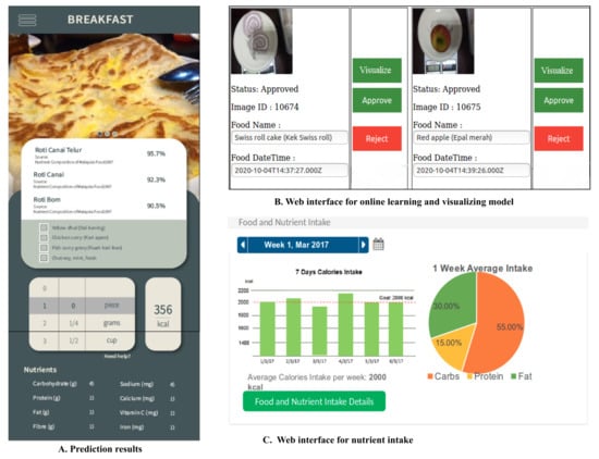
Figure 7.
Integration of the proposed framework with mobile application and web.
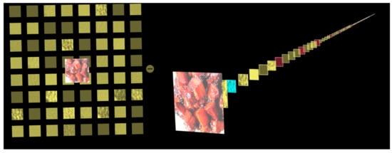
Figure 8.
3D visualization of category CNN by TensorSpace.
4.3. Performance Measures
We used Accuracy, Precision, Recall, and F1-score measures to compare classification performance. These measures are defined as follows:
4.3.1. Accuracy
It denotes the model’s ability to predict the food class accurately. Equation (41) represents its mathematical form.
Here, indicates false negative while represents false positive. Similarly, refers to true positive whilst refers to true negative.
4.3.2. F1-Score
The F1-score represents the weighted average of precision and recall, and it is represented by Equation (42). It considers both false positive and false negative by the model.
4.3.3. Recall
It is the model’s capability to classify the food classes correctly.
4.3.4. Precision
The precision score calculates the correctly classified positive values. It is computed by Equation (44):
Unlike food categorization, in which classification can be either correct or wrong. For food ingredient detection, PKELM may correctly classify several food ingredients and misclassifies other food ingredients, resulting in partial correctness of the classification. Therefore, we cannot directly employ evaluation metrics used to measure the classification performance of food categorization. This study uses the metrics based on the existing literature for multi-label classification. It uses Precision, Recall, and F1-score to measure performance. Consider with L number of labels as training datasets. Let assume MLC is the training method and is the output labels predicted by the classification method. Then these metrics are defined as follows:
4.3.5. Precision
Precision is the ratio of the predicted correct labels to the total number of actual labels, averaged across all instances. Equation (45) computes the precision.
4.3.6. Recall
It represents the ratio of predicted correct labels to the total number of predicted labels averaged over all the instances. Equation (46) computes the recall score.
4.3.7. F1-Score
F1-score is the harmonic mean of precision and recall and Equation (47) shows the mathematical expression.
Similarly, this study used five measures proposed by Kemker et al. [41] and Liew et al. [42] to measure catastrophic forgetting and stability of classifier during progressive growth of neurons and when the model adds new classes [1].
4.3.8. Intransigence
The intransigence of the network denotes the difference between the reference model and the incrementally trained model. The negative intransigence indicates that progressively learning up to k session is better than the batch method. Equation (48) denotes its mathematical form.
4.3.9. Forgetting
It is the difference between the maximum knowledge gained by the network in previous sessions and the existing session. Equation (49) computes the average forgetting of the network up to the session.
4.3.10. Base Session
It is the model’s performance on the base class data during the current session, and it is computed by Equation (50).
4.3.11. New Session
It is the model’s ability to recall newly learned knowledge and it is computed by the Equation (51).
4.3.12. All Session
It is the network performance on previously learned information while learning new knowledge as shown in Equation (52).
4.4. Results
4.4.1. Visual Features via Quality Resilient Convolutional Neural Network
We discussed above that this study selected InceptionResNetV2 for feature extraction as it gives the best discriminatory features in contrast to ResNet-50 and DenseNet-201. In the scenario of multilabel classification for ingredient detection, our framework has extracted feature vectors from the InceptionResNetV2 model fine-tuned using binary loss instead of categorical loss [1]. However, in the real-world environment, quality distortions in photos affect the robustness of features. This section discusses the results of the InceptionResNetV2 model under five common types of quality distortions in images to evaluate the effect on the robustness of the features. Secondly, it presents results of a comparison of classification performance on low-quality test images that shows fine-tuning CNN using the data augmentation strategy (RIMixUp) improves the robustness of CNN compared to the CNN fine-tuned with pristine food images. Then an explainable AI method, “Gradient Explainer” and t-distributed stochastic neighbor embedding (t-SNE) visualizations provide insight on how this data augmentation has improved the robustness of feature vectors extracted from the quality resilient CNN.
4.4.2. Impact of Food Image Quality on Visual Features from CNN
The experimental configurations are as follows. In case of contrast, the blending factor is varied from 0 to 1 in steps of 0.1. For Gaussian noise, the standard deviation is varied from 10 to 100. For Gaussian blur, it uses the Gaussian kernel and is varied from 1 to 15. For JPEG compression, the quality varies from 2 to 20, as above 20 JPEG compression does not impact the robustness of food features. The parameter of 100 represents an uncompressed JPEG image. For the defocus blur, the kernel size of the disk kernel is varied from 11 to 17. Figure 9 shows various distortions on randomly selected food images. Figure 10 shows the results of InceptionResnetNetV2 under various quality distortions. We observed that Gaussian noise and defocus blur have significantly reduced the robustness of features compared to other types of quality distortions. As JPEG compression does not affect performance above 20, it is useful for compressing images in real-time food recognition systems. We noted the worst effect of quality distortions for the VireoFood-172 dataset due to the low resolution of original images in the dataset. It reduces model performance by 50.28% for Gaussian blur at the kernel value of 3, by 18.67% for Gaussian noise at S.D of 20, and by 56.35% for defocus blur at disk kernel value of 11.
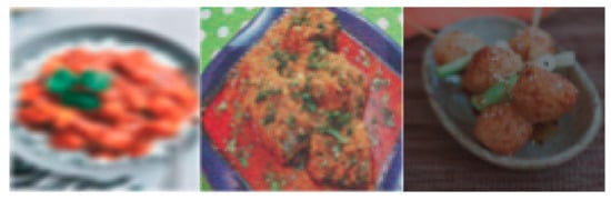
Figure 9.
Defocus blur, Gaussian noise and Gaussian blur on randomly selected images.
4.4.3. Random Iterative Mixup Data Augmentation during Fine-Tuning
The results in Figure 11 show that the proposed data augmentation strategy (RIMixUp) during fine-tuning improves the robustness of features extracted from the deep model. The robustness of feature vectors is at par in contrast to including all low-quality food images during fine-tuning. For the VireoFood-172 dataset, our data augmentation strategy improves performance by 16.81% for Gaussian noise, 44.46% for the Gaussian blur, and 48.47% for the defocus blur on low-quality test images as compared to model fine-tuned with pristine food images.
To further understand how the inclusion of low-quality images during transfer learning improves the robustness of features, we employed Gradient Explainer an explainable AI method to visualize the regions in an image and their contribution towards the top 3 most likely classes. We set the parameter rank_output to 3. Figure 12 and Figure 13A shows the visualization of a randomly selected image. The visualizations show that fine-tuning CNN without RIMixUp data augmentation strategy causes the same pixels or regions in the photo to activate for multiple classes especially Gaussian blur and defocus blur. It means that the quality distortions in the food photo increase overlapping amongst feature vectors extracted from CNN. However, Figure 12 and Figure 13C shows that the same set of pixels or regions are not activated for multiple classes when CNN has employed the RIMixUp data augmentation method during fine-tuning. It reduces overlapping among the features from images of various quality. To validate this, we extract the feature vectors from the model fine-tuned by using our data augmentation strategy, with low-quality images and model fine-tuned with pristine food images. t-SNE visualization of feature vectors in Figure 14 shows that the proposed data augmentation method for food images significantly reduces the overlapping among the feature vectors. Hence, making the feature extractor invariant to quality distortions. The results are similar when we include all low-quality images during transfer learning, even though fine-tuning with low-quality images increases the training time due to an increase in the size of the training dataset.

Figure 10.
InceptionResNetV2 under various quality distortions in the image: JPEG compression, Gaussian blur, Gaussian noise, and defocus blur.
Figure 10.
InceptionResNetV2 under various quality distortions in the image: JPEG compression, Gaussian blur, Gaussian noise, and defocus blur.


Figure 11.
Proposed data augmentation strategy RIMixUp during fine-tuning improves the robustness of the features.
Figure 11.
Proposed data augmentation strategy RIMixUp during fine-tuning improves the robustness of the features.


Figure 12.
Visualization of pristine and food photo with Gaussian noise shows our method activates the relevant pixels for correct class.
Figure 12.
Visualization of pristine and food photo with Gaussian noise shows our method activates the relevant pixels for correct class.


Figure 13.
Visualization of the food photo with Gaussian and defocus blur shows that using our strategy prevents the same set of pixels in the image to activate multiple classes.
Figure 13.
Visualization of the food photo with Gaussian and defocus blur shows that using our strategy prevents the same set of pixels in the image to activate multiple classes.


Figure 14.
t-SNE visualization shows overlapping among the feature vectors of low-quality images extracted (A) from the model fine-tuned with pristine images, (B) model fine-tuned using all low-quality images and (C) model fine-tuned using our proposed strategy.
Figure 14.
t-SNE visualization shows overlapping among the feature vectors of low-quality images extracted (A) from the model fine-tuned with pristine images, (B) model fine-tuned using all low-quality images and (C) model fine-tuned using our proposed strategy.

4.5. Gradient/Deep Explainer Based Strategy for Feature Selection
The feature vectors extracted from the InceptionResNetV2 have a very high dimension that leads to intractable workload and curse of dimensionality problem. However, developing a strategy for selecting an optimal subset of features is a challenge, as food recognition has many domain-specific challenges, such as no spatial layout information. We tackled this challenge by employing Gradient Explainer to visualize and understand the insight details. Figure 15 shows the red pixels have a positive contribution, and blue pixels have a negative contribution towards the most likely class. Similarly, for multilabel classification, Figure 16 shows that the SHAP values of the pixels from the visible portions of the ingredients in the food photo have a positive contribution towards the output. In the second common scenario, When the food ingredients are not visible in the image as shown in Figure 17. They are either hidden beneath the food or simply not visible. The SHAP values indicate that the model activates regions for various ingredients without any visually clear explanation. The key finding from our visualizations is that it shows the pixels from all the visually relevant regions in the food image do not contribute equally towards the desired category or ingredient. Following this idea, the proposed strategy selects the best features, with positive contributions towards the most likely food classes or food ingredients. We have selected the top 500 attributes from the feature vectors of the food images using our algorithm based on Deep Explainer and Gradient Explainer as in Algorithm 1. Table 4 shows the comparison of the classification performance on the PKELM classifier. It shows that the features selected by our method improve performance on the average of three trials in contrast to ReliefF. The reduction in training time for food category and ingredient detection (51.73%) is at par with the ReliefF method [1]. The advantage of the proposed feature selector is that it uses an explainable AI approach to analyze the importance of the features in contrast to classical techniques such as ReliefF, which do not have any visual explanations of selected features.
Table 4.
Comparison of average classification performance on incrementally trained classifier PKELM (RBF) by using different feature selection methods.
Table 4.
Comparison of average classification performance on incrementally trained classifier PKELM (RBF) by using different feature selection methods.
| Datasets | ReliefF | Deep Explainer | Gradient Explainer |
|---|---|---|---|
| Food101 | 85.54 | 85.09 | 86.05 |
| UECFOOD100 | 90.63 | 90.71 | 90.98 |
| UECFOOD256 | 75.85 | 79.56 | 79.34 |
| PFID | 100 | 100 | 100 |
| PFID-Baseline | 69.97 | 70.64 | 71.15 |
| Pakistani Food | 76.01 | 75.70 | 77.43 |
| VireoFood-172 | 91.88 | 91.97 | 92.09 |

Figure 15.
(A) Randomly selected image from Pakistani food dataset (B) Randomly selected image from UECFOOD256 dataset. Red pixels present the SHAP values of the image having a positive contribution towards the class while blue pixels show the pixels that reduce the probability of class.
Figure 15.
(A) Randomly selected image from Pakistani food dataset (B) Randomly selected image from UECFOOD256 dataset. Red pixels present the SHAP values of the image having a positive contribution towards the class while blue pixels show the pixels that reduce the probability of class.


Figure 16.
(A,B) Randomly selected images with visually visible ingredients. The visualization shows that the SHAP values of the pixels from the visible portions of the ingredients in the food image have the highest contribution towards the most likely outputs. By using ranked_outputs = 5 we explain only the five most likely ingredients. Bold indicates the actual ingredients.


Figure 17.
Red pixel shows the SHAP values that increase the probability of the ingredients. The blue pixels show the SHAP values that decreases the probability of the ingredients. By using ranked_outputs = 5 we explain only the five most likely ingredients.
Figure 17.
Red pixel shows the SHAP values that increase the probability of the ingredients. The blue pixels show the SHAP values that decreases the probability of the ingredients. By using ranked_outputs = 5 we explain only the five most likely ingredients.

4.6. Progressive Learning for Food Category and Ingredient Classification
After feature extraction and selection, PKELM learns incrementally from these feature vectors for classification. Figure 18 displays the randomly selected nodes and the nodes selected by PKELM. This section shows the results of the proposed PKELM to detect food categories and their corresponding ingredients compared to the state-of-the-art incremental extreme learning method. Finally, it discusses the results of catastrophic forgetting measures during the progression of mapping nodes and incremental learning.
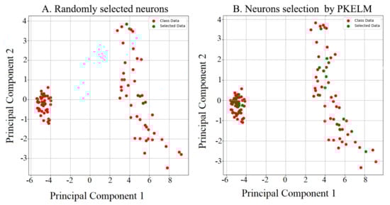
Figure 18.
(A) Randomly selected neurons and (B) Neuron selection by using PKELM from the first two training sessions during incremental learning of Pakistani food datasets.
4.6.1. Multi-Class Classification for Food Category
We implemented the incremental learning protocol proposed by Kemker et al. [41] and Liew et al. [42] to measure classification performance. There are two classes in the base session, and therefore, PKELM learns a novel class in every session. For batch classifiers such as ELM and RKELM, the study retrains the model on the whole dataset in every session. We presented average classification measures on the state-of-the-art ELM classifiers for each dataset. The kernel parameter is set to 0.1 in all the experiments, and ACIELM inserts hidden nodes when the error threshold is more than 0.8. For ARCIKELM, the fuzzy membership threshold value is set to zero during sequential learning like the original study [1]. We set the learning rate of PKELM through manual search [43] and presented the best results.
Table 5 shows the comparison of Top 1 and 3 percent classification accuracy, Precision, Recall, and F1-score across all six food datasets. All experiments are repeated three times for the same input sequence, and we have reported average accuracy. The experimental results show that PKELM performs better than ARCIKELM and other online variants of ELM. The improvement in accuracy for PKELM with RBF kernel in contrast to ARCIKELM for PFID baseline, UECFOOD100, UECFOOD256, Pakistani Food, and Food101 dataset is 4.12%, 1.78%, 0.49%, 2.8%, and 0.186%. For the VireoFood-172 dataset, the performance of both ARCIKELM and PKELM with RBF kernel is the same. It may be because VireoFood-172 has many images with fewer intra-class variations. PKELM with chi-square kernel improves classification accuracy as compared to ARCIKELM for PFID baseline, UECFOOD100, UECFOOD256, Pakistani Food, and Food101 dataset by 4.64%, 1.98%, 0.6%, 3.57%, and 0.84% respectively. It is worthy to note that the chi-square kernel in PKELM outperforms the RBF kernel for food categorization. The proposed classifier performs better than non-adaptive variants of ELM (batch methods) in terms of Accuracy, Precision, Recall, and F1-score on UECFOOD100, UECFOOD256, Pakistani Food Dataset, VireoFood-172, and the PFID baseline dataset.
Table 5.
Comparison of classification accuracy averaged over all sessions of the learning. If the precision and recall values in the session are not defined. Those values are denoted by 1 and are replaced by *.
The comparison of the Top 3 accuracy results shows that PKELM with RBF kernel improves performance in contrast to ARCIELM for UECFOOD256, UECFOOD100, PFID-baseline, and Pakistani food datasets by 0.13%, 1.08%, 1.57%, and 2.71%, respectively. For chi-square kernel in PKELM, it improves the Top 3 accuracy, in contrast to ARCIELM for UECFOOD256, UECFOOD100, PFID-baseline, and Pakistani food datasets by 0.99%, 1.91%, 1.8%, and 3.1% respectively. In contrast to all other online variants of ELM (CIELM and ACIELM), it has superior performance. Figure 19 presents the confusion matrix of PKELM. Figure 20 shows the ten best performing classes, worst classes, and most confused VireoFood-172 classes.
ACIELM has the worst performance for the top 1 and top 3 classifications, and it is consistent with the previous study as it suffers from high catastrophic forgetting during progressive learning. Ghalib et al. [1] stated that it is due to random input weights. We further suspect that sigmoid activation function in ACIELM also increases catastrophic forgetting during progression as it computes global representations.

Figure 19.
Comparison of each food category via the confusion matrix (x-axis and y-axis represent the number of classes) on the final PKELM model trained using the incremental learning protocol for all datasets (Best viewed under magnification).
Figure 19.
Comparison of each food category via the confusion matrix (x-axis and y-axis represent the number of classes) on the final PKELM model trained using the incremental learning protocol for all datasets (Best viewed under magnification).


Figure 20.
VireoFood-172 classification results (a) Worst performing classes (b) Confused classes (c) Best performing classes.
Figure 20.
VireoFood-172 classification results (a) Worst performing classes (b) Confused classes (c) Best performing classes.

4.6.2. Multi-Label Classification for Ingredient Detection
The study evaluated three food datasets with ingredient information for this experiment, VireoFood-172, Ingredient Food101 (Full), and Ingredient Food101 (Simplified). After feature extraction and selection, we implemented the incremental learning protocol proposed by kemker et al. [41] and Liew et al. [42] to measure performance. We categorize the unique set of labels into groups and set the kernel parameter to 0.1, and the learning rate in PKELM is set through manual search. In the base session, there are two groups. Following that, it learns a new group of ingredients in each session.
Experimental analysis in Table 6 shows that PKELM (RBF) has superior performance in contrast to InceptionResNetV2 and ResNet-50 for all datasets. For PKELM with RBF kernel, the difference in Precision, Recall, and F1-score for Food101 as compared to InceptionResnetV2 Model is (8.17%, 11.27%, 9.64%), Food101(Simplified) is (6.79%, 7.04%, 6.77%), and VireoFood-172 is (17.57%, 16.23%, 16.34%) respectively. When chi-square kernel is used in PKELM, the difference in Precision, Recall, and F1-score for Food101 as compared to InceptionResnetV2 Model is (6.35%, 6.70%, 5.61%), Food101(Simplified) is (7.42%, 1.48%, 2.46%), and VireoFood-172 is (19.10%, 13.05%, 14.99%), respectively. Figure 21 shows results of ingredient detection on randomly selected images.
Table 6.
Comparison of final measures of food ingredient recognition for Food101 and VireoFood-172 datasets.
Table 6.
Comparison of final measures of food ingredient recognition for Food101 and VireoFood-172 datasets.
| Datasets | Precision | Recall | F1-Score |
|---|---|---|---|
| Food101 | |||
| ResNet-50 | 83.42 | 59.34 | 69.35 |
| InceptionResNetV2 | 79.39 | 76.54 | 77.94 |
| PKELM (RBF) | 87.56 | 87.81 | 87.58 |
| PKELM (chi-squared) | 85.74 | 83.24 | 83.55 |
| Food101(Simplified) | |||
| ResNet-50 | 72.17 | 68.53 | 70.30 |
| InceptionResNetV2 | 76.10 | 76.41 | 76.25 |
| PKELM (RBF) | 82.89 | 83.45 | 83.02 |
| PKELM (chi-squared) | 83.52 | 77.89 | 78.71 |
| VireoFood-172 | |||
| ResNet-50 | 70.38 | 70.93 | 70.65 |
| InceptionResNetV2 | 70.40 | 70.94 | 70.67 |
| PKELM (RBF) | 87.98 | 87.18 | 87.02 |
| PKELM (chi-squared) | 89.51 | 84.00 | 85.67 |

Figure 21.
Results of ingredient detection on randomly selected images from the VireoFood-172 dataset.
Figure 21.
Results of ingredient detection on randomly selected images from the VireoFood-172 dataset.

4.7. Comparison of Catastrophic Forgetting during Progressive Learning
When the network adds new classes, catastrophic forgetting measures the retention of knowledge by the classifier. This section presented results of catastrophic forgetting of PKELM during progressive learning and compared it with other incremental classifiers of the extreme learning machine [1].
Similarly, like measuring classification performance, catastrophic forgetting is also regulated by the incremental learning protocol. In the base session, there are two classes, and each incoming session has one novel food category. All incremental classifiers are trained first on the base session data. For ACIELM, the error threshold parameter to insert the new nodes is 0.8. For ARCIKELM, the fuzzy membership threshold is kept zero, like in the original study [1]. In PKELM, we set the value of the kernel parameter to 0.1. Table 7 shows improvement in all sessions, the current session, and intransigence for the PFID-Baseline, Pakistani Food, UECFOOD100 and UECFOOD256 datasets. Similarly, it is worth noting that PFID-Baseline has large intraclass variation, which reduces ARCIKELM performance on base classes. On the other hand, PKELM dynamically computes the mapping nodes based on the activity value and handles the large intraclass variations. For the Food101 dataset, there is no significant difference noted between both classifiers. It may be due to fewer intra-class variations and many samples.
4.8. Novelty/Noise Detection during Online Learning
This section has discussed the results of the PKELM novelty detection mechanism for detecting the noising samples and for correctly assigning labels to unlabeled data instances during online learning. Figure 22 shows the samples images of non-food images in the dataset. We presented a well-trained model on the feature vectors from the UECFOOD100 dataset with 200 training instances. The data contains noisy samples. It consists of 150 feature vectors of food images and 50 feature vectors of non-food images. Figure 23 shows that the novelty detection mechanism correctly labels 131 feature vectors of food images as non-noisy samples. It wrongly labels 19 feature vectors of food images as noisy samples. Similarly, it correctly classifies 43 out of 50 feature vectors of non-food images as noisy instances before updating the model.
Table 7.
Comparison of average catastrophic forgetting measures during progressive learning for food category classification on each food dataset.
Table 7.
Comparison of average catastrophic forgetting measures during progressive learning for food category classification on each food dataset.
| Datasets | |||||
|---|---|---|---|---|---|
| PFID-Baseline | |||||
| CIELM | 0.3532 | 0.5441 | 0.5932 | 0.2532 | 0.1306 |
| ACIELM | 0.0022 | 0.1445 | 0.8234 | 0.8279 | 0.8359 |
| ARCIKELM | 0.0395 | 0.6618 | 0.7570 | 0.1794 | 0.0889 |
| PKELM (RBF) | 0.5391 | 0.8067 | 0.7860 | 0.1002 | 0.0986 |
| PKELM (chi-squared) | 0.5391 | 0.8074 | 0.7901 | 0.0950 | 0.0972 |
| Pakistani Food | |||||
| CIELM | 0.7905 | 0.7330 | 0.7492 | 0.0663 | 0.1044 |
| ACIELM | 0.4026 | 0.4605 | 0.9482 | 0.5481 | 0.5399 |
| ARCIKELM | 0.8044 | 0.7969 | 0.8289 | 0.0240 | 0.0848 |
| PKELM (RBF) | 0.7860 | 0.8253 | 0.8670 | −0.0169 | 0.0943 |
| PKELM (chi-squared) | 0.8863 | 0.8409 | 0.8646 | −0.0158 | 0.0934 |
| Food101 | |||||
| CIELM | 0.9069 | 0.8654 | 0.8695 | 0.0512 | 0.0575 |
| ACIELM | 0.4677 | 0.5688 | 0.9897 | 0.4642 | 0.5861 |
| ARCIKELM | 0.9430 | 0.9055 | 0.9078 | 0.0051 | 0.0417 |
| PKELM (RBF) | 0.9335 | 0.9042 | 0.9109 | 0.0056 | 0.0473 |
| PKELM (chi-squared) | 0.9412 | 0.9168 | 0.9244 | −0.0332 | 0.0620 |
| UECFOOD100 | |||||
| CIELM | 0.9500 | 0.9123 | 0.8319 | 0.0410 | 0.0688 |
| ACIELM | 0.3714 | 0.5450 | 0.9759 | 0.5240 | 0.6520 |
| ARCIKELM | 0.9642 | 0.9254 | 0.8651 | 0.0128 | 0.0512 |
| PKELM (RBF) | 0.9533 | 0.9363 | 0.8910 | −0.0005 | 0.0755 |
| PKELM (chi-squared) | 0.9557 | 0.9379 | 0.8861 | −0.0063 | 0.0563 |
| UECFOOD256 | |||||
| CIELM | 0.5362 | 0.7227 | 0.7757 | 0.1059 | 0.1236 |
| ACIELM | 0.1006 | 0.4722 | 0.9482 | 0.5481 | 0.5399 |
| ARCIKELM | 0.8808 | 0.8454 | 0.8691 | −0.0049 | 0.0839 |
| PKELM (RBF) | 0.8880 | 0.8491 | 0.8647 | −0.0332 | 0.0755 |
| PKELM (chi-squared) | 0.8109 | 0.8495 | 0.8810 | −0.0106 | 0.0876 |
The second experiment took 160 feature vectors of unlabeled feature vectors of food images. The objective is to assign labels based on the PKELM novelty detection mechanism during online learning. The classifier trained on the UECFOOD256 dataset has a mean threshold of 0.11031 and a standard deviation of 0.0985 on the training dataset. Figure 24 shows it assigns correct labels to 82 feature vectors of food images and mislabels two data inputs. It classified the remaining data instances as noisy samples, which means that the model does not have sufficient information to label them correctly.

Figure 22.
Samples of non-food images used in our experiments.
Figure 22.
Samples of non-food images used in our experiments.


Figure 23.
Activation values on network trained with UECFOOD100 dataset. Blue dots represent non-noisy food images. Orange dots represent food images classified as noisy samples. Grey dots show non-food images correctly determined as noisy samples. Yellow dots represent non-food images wrongly classified as non-noisy samples.


Figure 24.
Activation values on network trained with UECFOOD256 dataset with a test network of 200 food samples. Blue dots represent correctly labeled food images. Orange dots show mislabeled food images. Grey dots represent food images that are determined as noisy samples.
Figure 24.
Activation values on network trained with UECFOOD256 dataset with a test network of 200 food samples. Blue dots represent correctly labeled food images. Orange dots show mislabeled food images. Grey dots represent food images that are determined as noisy samples.

4.9. Comparison with Other Frameworks
We compared the classification performance of our framework with other states of the art methods. Our framework outperforms all the traditional approaches in terms of performance (SIFT, COLOR, PMTS, GTBB, PRICoLBP, etc.) [26] on all datasets. Moreover, none of these methods incrementally learn food classes and ingredients.
The deep learning approach Wiser-Net [44] has a better classification performance than our approach on UECFOOD100, UECFOOD256, and Food101 datasets, but it requires training of the network from scratch that requires long training time as compared to fine-tuning. Moreover, it cannot detect food ingredients, and like other CNN suffers from catastrophic forgetting during progressive learning. The comparison with CNN+INCEPTION [45], Ensemble Net [46] shows improvement in accuracy by 6.17% and 11.07% on the Food101 dataset. Although they trained both classifiers by using a batch learning protocol. For the UECFOOD100 and UECFOOD256 datasets, it improves accuracy as compared to CNN [47] by (2.74%, 1.69%), and CNN+INCEPTION [45] by (5.24%, 14.59%) while incrementally learning new categories and ingredients in the food. Similarly, compared to SELC [26] architecture, the improvement in accuracy on the PFID dataset is 7.16%, and the Food101 dataset is 27.28%. The KELM classifier in SELC is non-adaptive. It cannot incrementally learn new classes, and it uses a batch protocol for model training. The framework enhances accuracy by 4.19% for the category and by 20.81% for ingredients recognition as compared to the Arch-D [24] architecture. The comparison with the incremental classifier ARCIKELM by Ghalib et al. [1] shows that classification performance is improved for UECFOOD100 by 2.24%, UECFOOD256 by 2.83%, and 4.5% for the Pakistani Food dataset. The comparison with SPC [25] (personalized incremental classifier) shows that SPC is unable to detect ingredients or malicious images during online learning. As it is a personalized framework, the authors did not evaluate their model on standard benchmarks. Table 8 and Table 9 summarizes the comparison for the food category classification dataset. Table 10 shows the comparison for ingredient detection with other methods.
Table 8.
Summary of research using deep feature extraction and fine-tuning methods to classify the Food101 dataset.
Table 9.
Summary of research using deep feature extraction and fine-tuning to classify the UECFOOD256 dataset.
Table 10.
Result of comparison with other methods of ingredient detection for VireoFood-172 dataset.
5. Discussion
Based on the extensive analysis carried out for this research work, we can state the following considerations. For feature extraction, although, the CNN model has given discriminatory features. However, various quality distortions in the images impact the robustness of features as observed in Figure 10. Fine-tuning the network by using our proposed data augmentation “random iterative mixup” improves the robustness of feature vectors extracted from the deep model by reducing the impact of distortions as shown in Figure 11. Our proposed augmentation method does not increase the training set size or training time compared to fine-tuning with low-quality images. It also inherits the benefits of mixup and is extremely good at regularizing deep models. To the best of our knowledge, it is the first detailed work to evaluate the impact of quality distortions and tackled this challenge for food datasets. Despite advantages, we have not evaluated our method at extreme quality distortions as such distortions occur rarely in the photo captured by using modern smartphone cameras.
In the second step, we selected the optimal subset of quality resilient features from the high dimension space. Due to the absence of a rigid structure of the food, selecting the optimal subset of features is a problem. We tackle this problem by employing the Gradient Explainer strategy to understand the contribution of an area of interest in food images towards the output layer. Our visualization by Gradient Explainer in Figure 15, Figure 16 and Figure 17 shows that all pixels in the food image do not contribute equally or positively towards the most likely class. Based on these findings, we proposed a novel strategy that uses the SHAP values from the gradient explainer method to rank the features. Our method selects the top 500 most relevant features by filtering out irrelevant ones. For food category and ingredient detection, the accumulated training time is reduced by 51.73%. It is also observed in Table 4 that it improves the performance of the classifier as compared to ReliefF.
Following feature extraction and selection, we employed the progressive classifier PKELM for food categorization and ingredient detection. It successfully replaced the random selection of nodes in ARCIKELM [1] by activity value for the progression of mapping nodes. To extend PKELM for multi-label classification, we employed the bipolar step function to process test output and then selected the column labels of the resulting matrix with value one. The food categorization results on the standard benchmarks show that PKELM improves classification performance for UECFOOD100 by 2.24%, UECFOOD256 by 2.83%, and 4.5% for the Pakistani Food dataset as compared to ARCIEKLM and ReliefF by Ghalib et al. [1]. For ingredient detection, PKELM improves performance on Food101, Food101(Simplified), and VireoFood-172 datasets by 8.17%, 6.79%, and 17.57% as compared to the deep learning model. Moreover, it is noteworthy that the classifier learns progressively. The investigation based on catastrophic forgetting measures shows that our classifier is stable during progressive learning and retains the previous knowledge. During online learning, it tackles domain changes due to quality distortions, changes in concepts, etc., by remodeling its structure compared to existing batch methods. Moreover, our results in Figure 23 and Figure 24 show that our novelty detection mechanism can detect noisy data samples and can assigns labels to unlabeled data instances. The detailed comparison with other works in our “comparison sections” indicates that the proposed framework is better on many scales.
6. Conclusions
Food logging applications using vision-based methods for food recognition face several challenges outside the laboratory environment. Firstly, deep networks trained on pristine food images have a poor performance on distorted images affected by blur or additive noise during image acquisition. Similarly, progressive learning is vital for catering to domain variations due to quality distortions or changes in concepts. Despite that, existing progressive classifiers recognize food categories and do not detect food ingredients. We have designed a quality resilient explainable framework by keeping in view the challenges faced by the practical food logging applications. It uses the state-of-the-art deep learning model (InceptionResNetV2) for feature extraction. To study the effect of image quality on it, we have examined the model under various quality distortions. Based on our analysis, we have successfully improved the robustness of the convolutional neural network by using our novel data augmentation method, RIMixUp, during fine-tuning. The experimental results have shown a significant improvement in the robustness of visual features extracted via quality resilient CNN.
After visual feature extraction via the quality resilient convolutional neural network, we have tackled the challenge of selecting the optimal subset of features from high dimension feature space. At first, we have used the Gradient Explainer to understand the contribution of the photo pixels and the area of interest to the output layer. These visualizations have shown that all pixels from the relevant portions do not have an equal or positive contribution. Based on these findings, the Gradient Explainer-based algorithm uses SHAP values to rank features and then selects reliable attributes from high dimensional data. This strategy has shown improved performance and has reduced the accumulated learning time of the PKELM classifier by 51.73% for all the food datasets.
During the classification stage, our work has used a progressive classifier—PKELM—to categorize food and ingredient detection. It has dynamically adjusted its structure using the activation value to cater to domain changes and novel concepts. Moreover, unlike most previous works, it has learned both food categories and ingredients. During online learning, it has detected noisy instances and has assigned labels to unlabeled data instances.
Experimental analysis of our framework has shown the competitive performance as compared to other works while having many technical advantages for practical food logging applications. To the best of our knowledge, it is the first framework that has tackled low-quality food images, has detected noisy instances during online learning, and has assigned labels to unlabeled data instances. Similarly, in contrast to other methodologies, it has employed a progressive classifier for food categorization and ingredient detection. Finally, we have integrated the framework with a mobile application to automate food image analysis.
In the future, we plan to conduct research in three directions: (1) We plan to exploit unsupervised feature learning, as preparing a large comprehensive annotated dataset is a challenge; (2) We can reduce the classification space in a practical application by incorporating personal dietary preferences such as vegetarian, non-vegetarian. This approach would presumably simplify and improve the classification performance of the proposed framework; and (3) We generalize the proposed framework to other related fields such as fruits and plant disease detection and so forth.
Author Contributions
G.A.T. was responsible for writing algorithms, analysis, writing the article and literature search, and approved the final version as submitted. C.K.L. contributed to the study design, reviewed the study for intellectual content, and confirmed the final version as submitted. All authors have read and agreed to the published version of the manuscript.
Funding
This research was supported by the University Malaya Impact-oriented Interdisciplinary Research Grant Programme (IIRG)-IIRG002C-19HWB, University Malaya Covid-19 Related Special Research Grant (UMCSRG) CSRG008-2020ST, and Partnership Grant (RK012-2019) from University Malaya.
Institutional Review Board Statement
Not applicable.
Informed Consent Statement
Not applicable.
Conflicts of Interest
The authors declare there is no conflict of interest.
References
- Tahir, G.A.; Loo, C.K. An Open-Ended Continual Learning for Food Recognition Using Class Incremental Extreme Learning Machines. IEEE Access 2020, 8, 82328–82346. [Google Scholar] [CrossRef]
- Urbanowicz, R.J.; Meeker, M.; La Cava, W.; Olson, R.S.; Moore, J.H. Relief-based feature selection: Introduction and review. J. Biomed. Inform. 2018, 85, 189–203. [Google Scholar] [CrossRef] [PubMed]
- Herranz, L.; Xu, R.; Jiang, S.; Luis, H. A probabilistic model for food image recognition in restaurants. In Proceedings of the 2015 IEEE International Conference on Multimedia and Expo (ICME), Turin, Italy, 29 June–3 July 2015; pp. 1–6. [Google Scholar] [CrossRef]
- Wanjeka, P.; Narongwut, K.; Rattapoom, W. Automatic sushi classification from images using color histograms and shape properties. In Proceedings of the 2014 3rd ICT International Senior Project Conference, ICT-ISPC 2014, Bangkok, Thailand, 26–27 March 2014; pp. 83–86. [Google Scholar] [CrossRef]
- Kong, F.; Tan, J. DietCam: Automatic dietary assessment with mobile camera phones. Pervasive Mob. Comput. 2012, 8, 147–163. [Google Scholar] [CrossRef]
- Anthimopoulos, M.M.; Gianola, L.; Scarnato, L.; Diem, P.; Mougiakakou, S.G. A Food Recognition System for Diabetic Patients Based on an Optimized Bag-of-Features Model. IEEE J. Biomed. Health Inform. 2014, 18, 1261–1271. [Google Scholar] [CrossRef]
- Zheng, J.; Wang, Z.J.; Ji, X. Superpixel-based image recognition for food images. In Proceedings of the 2016 IEEE Canadian Conference on Electrical and Computer Engineering (CCECE), Vancouver, BC, Canada, 15–18 May 2016; pp. 1–4. [Google Scholar] [CrossRef]
- Miyano, R.; Uematsu, Y.; Saito, H. Food region detection using bag-of-features representation and color feature. In Proceedings of the International Conference on Computer Vision Theory and Applications, VISAPP 2012, Rome, Italy, 24–26 February 2012; pp. 709–713. [Google Scholar]
- Nguyen, D.T.; Zong, Z.; Ogunbona, P.O.; Probst, Y.; Li, W. Food image classification using local appearance and global structural information. Neurocomputing 2014, 140, 242–251. [Google Scholar] [CrossRef]
- Farinella, G.M.; Allegra, D.; Moltisanti, M.; Stanco, F.; Battiato, S. Retrieval and classification of food images. Comput. Biol. Med. 2016, 77, 23–39. [Google Scholar] [CrossRef]
- Pouladzadeh, P.; Shirmohammadi, S.; Arici, T.; Arici, T. Intelligent SVM based food intake measurement system. In Proceedings of the 2013 IEEE International Conference on Computational Intelligence and Virtual Environments for Measurement Systems and Applications (CIVEMSA), Milan, Italy, 15–17 July 2013; pp. 87–92. [Google Scholar] [CrossRef]
- Matsuda, Y.; Yanai, K. Multiple-food recognition considering co-occurrence employing manifold ranking. In Proceedings of the 21st International Conference on Pattern Recognition (ICPR2012), Tsukuba, Japan, 11–15 November 2012; pp. 2017–2020. [Google Scholar]
- Bettadapura, V.; Thomaz, E.; Parnami, A.; Abowd, G.D.; Essa, I. Leveraging Context to Support Automated Food Recognition in Restaurants. In Proceedings of the 2015 IEEE Winter Conference on Applications of Computer Vision, Waikoloa, HI, USA, 5–9 January 2015; pp. 580–587. [Google Scholar] [CrossRef]
- Kusumoto, R.; Han, X.; Chen, Y.-W. Hybrid Aggregation of Sparse Coded Descriptors for Food Recognition. In Proceedings of the 2014 22nd International Conference on Pattern Recognition, Stockholm, Sweden, 24–28 August 2014; pp. 1490–1495. [Google Scholar] [CrossRef]
- He, H.; Kong, F.; Tan, J. DietCam: Multiview Food Recognition Using a Multikernel SVM. IEEE J. Biomed. Health Inform. 2015, 20, 848–855. [Google Scholar] [CrossRef]
- Luo, Y.; Ling, C.; Ao, S. Mobile-based food classification for Type-2 Diabetes using nutrient and textual features. In Proceedings of the 2014 International Conference on Data Science and Advanced Analytics (DSAA), Shanghai, China, 30 October–2 November 2014; pp. 563–569. [Google Scholar] [CrossRef]
- Tanno, R.; Okamoto, K.; Yanai, K. DeepFoodCam: A DCNN-based Real-time Mobile Food Recognition System. In Proceedings of the 2nd International Workshop on Multimedia Assisted Dietary Management, Amsterdam, The Netherlands, 16 October 2016; pp. 89–89. [Google Scholar] [CrossRef]
- Liu, C.; Cao, Y.; Luo, Y.; Chen, G.; Vokkarane, V.; Yunsheng, M.; Chen, S.; Hou, P. A New Deep Learning-Based Food Recognition System for Dietary Assessment on An Edge Computing Service Infrastructure. IEEE Trans. Serv. Comput. 2017, 11, 249–261. [Google Scholar] [CrossRef]
- Meyers, A.; Johnston, N.; Rathod, V.; Korattikara, A.; Gorban, A.; Silberman, N.; Guadarrama, S.; Papandreou, G.; Huang, J.; Murphy, K.P. Im2Calories: Towards an Automated Mobile Vision Food Diary. In Proceedings of the 2015 IEEE International Conference on Computer Vision (ICCV), Santiago, Chile, 7–13 December 2015; pp. 1233–1241. [Google Scholar] [CrossRef]
- Sahoo, D.; Hao, W.; Ke, S.; Wu, X.W.; Le, H.; Achananuparp, P.; Lim, E.-P.; Hoi, S.C.H. FoodAI: Food Image Recognition via Deep Learning for Smart Food Logging. In Proceedings of the 25th ACM SIGKDD International Conference on Knowledge Discovery & Data Mining, Anchorage, AK, USA, 4–8 August 2019; pp. 2260–2268. [Google Scholar] [CrossRef]
- Ciocca, G.; Napoletano, P.; Schettini, R. Food Recognition: A New Dataset, Experiments, and Results. IEEE J. Biomed. Health Inform. 2016, 21, 588–598. [Google Scholar] [CrossRef]
- Heravi, E.J.; Aghdam, H.H.; Puig, D. Classification of Foods Using Spatial Pyramid Convolutional Neural Network. Artificial Intelligence Research and Development. In Proceedings of the 19th International Conference of the Catalan Association for Artificial Intelligence, Barcelona, Spain, 19–21 October 2016; Volume 288, pp. 163–168. [Google Scholar]
- Jiang, S.; Min, W.; Liu, L.; Luo, Z. Multi-Scale Multi-View Deep Feature Aggregation for Food Recognition. IEEE Trans. Image Process. 2019, 29, 265–276. [Google Scholar] [CrossRef]
- Chen, J.; Ngo, C.-W. Deep-based Ingredient Recognition for Cooking Recipe Retrieval. In Proceedings of the 24th ACM International Conference on Multimedia (MM’16), Amsterdam, The Netherlands, 15–19 October 2016; Association for Computing Machinery: New York, NY, USA, 2016; pp. 32–41. [Google Scholar] [CrossRef]
- Horiguchi, S.; Amano, S.; Ogawa, M.; Aizawa, K. Personalized Classifier for Food Image Recognition. IEEE Trans. Multimedia 2018, 20, 2836–2848. [Google Scholar] [CrossRef]
- Martinel, N.; Piciarelli, C.; Micheloni, C. A supervised extreme learning committee for food recognition. Comput. Vis. Image Underst. 2016, 148, 67–86. [Google Scholar] [CrossRef]
- Dodge, S.; Karam, L. Understanding how image quality affects deep neural networks. In Proceedings of the 2016 Eighth International Conference on Quality of Multimedia Experience (QoMEX), Lisbon, Portugal, 6–8 June 2016; pp. 1–6. [Google Scholar] [CrossRef]
- Zhang, L.; Deng, Z.; Kawaguchi, K.; Ghorbani, A.; Zou, J.Y. How Does Mixup Help With Robustness and Generalization? arXiv 2021, arXiv:2010.04819. [Google Scholar]
- Zhang, H.; Cissé, M.; Dauphin, Y.; Lopez-Paz, D. mixup: Beyond Empirical Risk Minimization. arXiv 2018, arXiv:1710.09412. [Google Scholar]
- Borkar, T.S.; Karam, L.J. DeepCorrect: Correcting DNN Models Against Image Distortions. IEEE Trans. Image Process. 2019, 28, 6022–6034. [Google Scholar] [CrossRef]
- Zheng, S.; Song, Y.; Leung, T.; Goodfellow, I. Improving the Robustness of Deep Neural Networks via Stability Training. In Proceedings of the IEEE Conference on Computer Vision and Pattern Recognition, Las Vegas, NV, USA, 27–30 June 2016. [Google Scholar] [CrossRef]
- Sun, Z.; Ozay, M.; Zhang, Y.; Liu, X.; Okatani, T. Feature Quantization for Defending Against Distortion of Images. In Proceedings of the 2018 IEEE/CVF Conference on Computer Vision and Pattern Recognition, Salt Lake City, UT, USA, 18–23 June 2018; pp. 7957–7966. [Google Scholar] [CrossRef]
- Lundberg, S.M.; Lee, S. A unified approach to interpreting model predictions. In Proceedings of the 31st International Conference on Neural Information Processing Systems (NIPS’17), Long Beach, CA, USA, 4–9 December 2017; Curran Associates Inc.: Red Hook, NY, USA, 2017; pp. 4768–4777. [Google Scholar]
- Marsland, S.; Shapiro, J.; Nehmzow, U. A self-organising network that grows when required. Neural Netw. 2002, 15, 1041–1058. [Google Scholar] [CrossRef]
- Rasmussen, C.E.; Williams, C.K.I. Gaussian Processes for Machine Learning; The MIT Press: Cambridge, MA, USA, 2006. [Google Scholar]
- Zhang, J.; Marszalek, M.; Lazebnik, S.; Schmid, C. Local Features and Kernels for Classification of Texture and Object Categories: A Comprehensive Study. In Proceedings of the 2006 Conference on Computer Vision and Pattern Recognition Workshop (CVPRW’06), New York, NY, USA, 17–22 June 2006; p. 13. [Google Scholar] [CrossRef]
- Bossard, L.; Guillaumin, M.; Van Gool, L. Food-101—Mining Discriminative Components with Random Forests. In Proceedings of the European Conference on Computer Vision, Zurich, Switzerland, 6–12 September 2014; pp. 446–461. [Google Scholar] [CrossRef]
- Bolaños, M.; Ferrà, A.; Radeva, P. Food Ingredients Recognition Through Multi-label Learning. In New Trends in Image Analysis and Processing—ICIAP 2017; Lecture Notes in Computer Science; Battiato, S., Farinella, G., Leo, M., Gallo, G., Eds.; Springer: Cham, Switzerland, 2017; Volume 10590. [Google Scholar] [CrossRef]
- Kawano, Y.; Yanai, K. Automatic Expansion of a Food Image Dataset Leveraging Existing Categories with Domain Adaptation. In Proceedings of the European Conference on Computer Vision, Zurich, Switzerland, 6–12 September 2014; pp. 3–17. [Google Scholar] [CrossRef]
- Chen, M.; Dhingra, K.; Wu, W.; Yang, L.; Sukthankar, R.; Yang, J. PFID: Pittsburgh fast-food image dataset. In Proceedings of the 2009 16th IEEE International Conference on Image Processing (ICIP), Cairo, Egypt, 7–10 November 2009; pp. 289–292. [Google Scholar] [CrossRef]
- Kemker, R.; McClure, M.; Abitino, A.; Hayes, T.; Kanan, C. Measuring Catastrophic Forgetting in Neural Networks. arXiv 2017, arXiv:1708.02072. [Google Scholar]
- Liew, W.S.; Loo, C.K.; Gryshchuk, V.; Weber, C.; Wermter, S. Effect of Pruning on Catastrophic Forgetting in Growing Dual Memory Networks. In Proceedings of the 2019 International Joint Conference on Neural Networks (IJCNN), Budapest, Hungary, 14–19 July 2019; pp. 1–8. [Google Scholar] [CrossRef]
- Feurer, M.; Hutter, F. Hyperparameter Optimization. In Automated Machine Learning; The Springer Series on Challenges in Machine Learning; Hutter, F., Kotthoff, L., Vanschoren, J., Eds.; Springer: Cham, Swizerland, 2019. [Google Scholar] [CrossRef]
- Martinel, N.; Foresti, G.L.; Micheloni, C. Wide-Slice Residual Networks for Food Recognition. In Proceedings of the 2018 IEEE Winter Conference on Applications of Computer Vision (WACV), Lake Tahoe, NV, USA, 12–15 March 2018; pp. 567–576. [Google Scholar] [CrossRef]
- Liu, C.; Cao, Y.; Luo, Y.; Chen, G.; Vokkarane, V.; Ma, Y. DeepFood: Deep Learning-Based Food Image Recognition for Computer-Aided Dietary Assessment. In Inclusive Smart Cities and Digital Health; ICOST 2016, Lecture Notes in Computer Science; Chang, C., Chiari, L., Cao, Y., Jin, H., Mokhtari, M., Aloulou, H., Eds.; Springer: Cham, Swizerland, 2016; Volume 9677. [Google Scholar] [CrossRef]
- Pandey, P.; Deepthi, A.; Mandal, B.; Puhan, N.B. FoodNet: Recognizing Foods Using Ensemble of Deep Networks. IEEE Signal Process. Lett. 2017, 24, 1758–1762. [Google Scholar] [CrossRef]
- Yanai, K.; Kawano, Y. Food Image Recognition Using Deep Convolutional Network with Pre-Training and Fine-Tuning. In Proceedings of the 2015 IEEE International Conference on Multimedia & Expo Workshops (Icmew), Turin, Italy, 29 June–3 July 2015; pp. 1–6. [Google Scholar] [CrossRef]
- McAllister, P.; Zheng, H.; Bond, R.; Moorhead, A. Combining deep residual neural network features with supervised machine learning algorithms to classify diverse food image datasets. Comput. Biol. Med. 2018, 95, 217–233. [Google Scholar] [CrossRef]
- Mandal, B.; Puhan, N.B.; Verma, A. Deep Convolutional Generative Adversarial Network-Based Food Recognition Using Partially Labeled Data. IEEE Sens. Lett. 2019, 3, 7000104. [Google Scholar] [CrossRef]
- Liu, C.; Liang, Y.; Xue, Y.; Qian, X.; Fu, J. Food and Ingredient Joint Learning for Fine-Grained Recognition. IEEE Trans. Circuits Syst. Video Technol. 2021, 31, 2480–2493. [Google Scholar] [CrossRef]


Publisher’s Note: MDPI stays neutral with regard to jurisdictional claims in published maps and institutional affiliations. |
© 2021 by the authors. Licensee MDPI, Basel, Switzerland. This article is an open access article distributed under the terms and conditions of the Creative Commons Attribution (CC BY) license (https://creativecommons.org/licenses/by/4.0/).