1. Introduction
Due to the growing need for reducing air pollution and, at the same time, offering mobility services of satisfactory quality to citizens, new means of urban mobility are being explored in many large cities around the world. Bike-sharing systems (BSSs) are just one of the many solutions that have been proposed and implemented in recent years. In some cities, they have grown to considerable size. For example, the system Vélib (
http://www.velib-metropole.fr/) in Paris has ~15,000 bikes, the Santander Cycles project in London (
tfl.gov.uk/modes/cycling/santander-cycles) has ~11,000 bikes and cities in China such as Hangzhou or Wuhan employ as many as 78,000 and 90,000 bikes, respectively [
1]. Some of those systems are so called free-floating systems (e.g.,
BikeShare in Seattle or DB
Callabike in Munich) that allow citizens to pick up and return a bike at any location within a certain area. Others are station-based—that is, they rely on a set of rental stations with fixed locations. Station-based BSSs have the advantage of providing better control to avoid unauthorized access. When electric bikes are deployed in the BSS—as, for example, in the BiciMAD system in Madrid (Spain)—stations usually serve as charging spots for the bicycles’ batteries as well.
Effectiveness and user satisfaction within station-based BSSs strongly depend on the availability of bikes (or slots for returning rented bikes) at the places where users search for them or demand them. Therefore, proper management policies need to be implemented not only for strategic decisions (e.g., regarding the positioning and dimensioning of rental stations, the selection of adequate bicycle models, etc.), but also at the operational level. In particular, BSSs are usually faced with agglomeration or unbalancing problems: available bikes are concentrated at certain areas (and at certain times of the day), whereas in other areas few or no bikes are available. The effect is that users may experience a poor quality of service, being unable to find a bike (or a return slot) at a given station or area. Solutions such as reserving bikes (or slots) at some stations palliate this problem, but proper bike balancing mechanisms are needed in order to tackle the problem at its core.
In many systems, trucks are used to address such balancing problems, by moving bicycles from (almost) full to (almost) empty stations. Truck movements are scheduled either statically (usually at night) or dynamically (during BSS operation), with the aim of finding a near-optimal match between the expected demand and the available resources. However, truck movements are expensive, and raise environmental concerns.
Today, BSSs are often conceived as cyber–physical systems [
2,
3]. Bikes may be endowed with several battery-powered sensors that measure important information such as position or battery level (in case of electric bicycles). Sensors at stations may capture rental attempts that were frustrated—e.g., due to mechanical failures of slot clamps—and, of course, gather key information regarding the operating state of the system, such as the numbers of available and occupied slots. This information is then transmitted to a software application at the BSS control centre, and helps operators to make timely management decisions in an online manner. Part of this information is often shared with the BSS users, who may use smartphone apps that inform them about the current state of stations in real time. Users can then use this information to make more informed decisions as to where to rent or to return a bike. However, due to the dynamic nature of the BSS environment, it often transpires that, when a user reaches a certain station, initially available bikes have already been taken by other users. Similarly, information on available parking slots may already be outdated when a user arrives to a station. Dynamic reservation schemes can be used to address such problems, but may have a negative impact on the overall capacity of a BSS.
BSSs are also often perceived from the perspective of the smart cities paradigm as part of a more sophisticated, heterogeneous, intelligent transportation solution—a system of systems that integrates different modes of transport (buses, trains, private and shared vehicles, on-demand transportation services, etc.) and enables dynamic collaborations among users, such as crowdshipping [
4] or crowdsensing [
5,
6] scenarios. In a multimodal context [
7,
8], real-time recommendation systems may suggest any type of appropriate means of transport (not just bikes) that fits the particular needs and preferences of a user at a particular moment. In some cases, this may alleviate the quality of service problems within a BSS due to imbalances, as mentioned above. For example, if there are no available bikes in the area of a user, the system may recommend an on-demand shared taxi service, instead of walking to another BSS station. This perspective is very appealing, and research in this direction will pave the way towards better and greener transportation services in smart cities [
9,
10]; however, it does not explicitly account for the agglomeration problems that reduce the quality of service at the level of the BSS. Therefore, we argue that addressing the imbalance problem in BSSs is still a relevant endeavour, as it can impact positively on the overall service level of intelligent transportation systems within a smart city.
In this work, we focus on the aforementioned problems within station-based BSSs. Our first contribution is a novel recommendation strategy based on a notion of cost that combines distance (between a user’s origin/destination and a rental/return station) with (an expectation of) availability of slots or bikes. To account for the dynamic nature of the BSS environment as mentioned earlier, instead of recommending stations that have available bikes or slots at the time a search request is made, we use demand prediction to estimate the expected probability of finding an available bike or slot at the time the user will arrive at a recommended station. In particular, we model stations as queues, and apply techniques from queuing theory for probability estimation.
The second contribution of this work is an extension of the aforementioned recommendation strategy that also addresses balancing problems by combining individual objectives with social welfare. For this purpose, the system not only tries to recommend stations with a low cost for the user, but also uses demand predictions to estimate the impact of renting or returning a bike at a given station on society (potential future users). Here, recommendations prioritise stations (for rental or return actions) that combine a low cost for the user with an improved overall impact on the distribution of bikes and slots in the BSS (and, thus, for potential future users).
To evaluate the proposed recommendation strategies, we used a simulation tool for station-based bike-sharing systems: Bike3S (
https://github.com/gia-urjc/Bike3S-Simulator). This simulator performs semi-realistic simulations of the operation of a bike-sharing system in a given area of interest, and allows for evaluating and testing different management decisions and strategies. In our simulations, we used real data from the BiciMAD BSS, which is operating in Madrid (Spain).
The rest of the paper is organised as follows: In
Section 2 we discuss related works on bicycle-sharing systems.
Section 3 outlines the general functioning of a station-based BSS, and introduces the basic notation used in the rest of the paper.
Section 4 focuses on station recommendation strategies that are centred on BSS users. In particular, we sketch some simple, straightforward selection strategies, before introducing our more sophisticated proposal.
Section 5 puts forward several experiments that compare the performance of the different strategies. In
Section 6, we present our estimation of the impact of a rental/return action at a station on potential future users, and define our proposal for a station recommendation strategy that combines cost for users and future global impact. In
Section 7, we analyse the performance of this strategy in a set of simulation experiments. Finally,
Section 8 summarises our work, outlines the lessons we have learned, and points to future lines of work.
2. Related Work
Bike-sharing systems’ management decisions can be made with different temporal horizons.
Long-term or
strategic decisions are mainly related to system design and deployment (location and size of stations, number of bikes, etc.) [
11,
12,
13,
14], as well as the analysis of different exploitation policies for existing systems [
15].
At an
operational level, decisions are made in order to maintain a good performance of the system, which usually means maximizing the number of users that rent bikes. Thus, actions are aimed at reducing imbalances produced at stations due to heterogeneous demand for bikes and empty slots. In this regard,
offline or static approaches are mid-term decisions oriented at repositioning bikes using vehicles (trucks)—typically at night, or during off-peak times—in such a way that bike distribution through stations is optimal for the expected demand. These systems estimate the best way of distributing not only the existing bikes, but also the routes taken by the trucks (see e.g., [
16,
17,
18]).
A natural evolution of such systems is their
online application during the actual operation of the fleet. The challenge is in combining the current state of the system with demand prediction, so as to propose short-term balancing actions. Many works propose solutions to the problem of dynamically repositioning bikes using trucks as efficiently as possible [
19,
20,
21,
22]. It has become clear that optimal solutions to the optimization problem do not scale as the size of the BSS grows, so authors use heuristics to find solutions applicable in real-world systems.
Furthermore, using trucks to rebalance a bike-sharing fleet has several disadvantages, including cost of operation, contribution to congestion and pollution, etc. Recently, several approaches have proposed crowdsourcing this task, so that users can contribute by taking or returning bikes at stations other than their target station. Typically, users receive some type of incentive (e.g., discounts) to compensate the extra (usually small) effort of modifying their initial choices.
This paper focuses on dynamic rebalancing systems; thus, we describe related works in this area in further detail.
Chemla et al. [
19] studied the problem of obtaining the optimal policy to determine the best action that a repositioning vehicle can take in order to maximise the number of users that find a bike. Since this is an NP-hard problem, they proposed several heuristic solutions that, roughly speaking, are based on choosing the station with the most or least excess of bikes with regard to a given target state. They also employed a pricing strategy in which each station has a price that is paid when the bike is returned, regardless of the origin of the trip; users choose the destination station based on its current price and the user’s walking and biking distances. This solution consists of optimizing station prices assuming certain user models.
Pfrommer et al. [
23] presented a dynamic rebalancing system that combines truck-based vehicle redistribution and price incentives for users. In this approach, users either find a bike at their origin stations or leave the system. Upon arrival at their target station, users decide whether or not to accept an incentive to return the bike at a neighbouring station. This decision is taken according to their “perceived cost” of the additional distance travelled (biking and walking) and the incentives received. Dynamic prices are calculated through an optimization problem that combines the quality of the resulting state and the cost of paying out the incentives. The key component of the system quality is the analysis of each station’s utility, based on an optimal “fill level” (the available bikes at a station).
Haider et al. [
24] proposed a method that combines trucks and price incentives. In this approach, the authors intentionally tried to make some stations even more imbalanced (hubs), so that bike redistribution could be carried out more efficiently with shorter truck trips. The objective was to minimize the number of imbalanced stations, which the authors solved heuristically. Prices (which include incentives) were established for O–D station pairs.
Singla et al. [
25] presented a mechanism that incentivizes the users in the bike repositioning process; they employed optimal pricing policies using regret minimization in online learning, and investigated the incentive compatibility of their mechanism. This approach was evaluated through simulations based on historical data from the Boston Hubway system, as well as on data collected via a survey study with MVGmeinRad in Mainz, Germany.
Reiss and Bogenberger [
26] proposed a hybrid approach for a free-floating bike-sharing system in which user discounts (60–100%) are applied when the imbalance is low (less than 15%), or trucks are used in case of high imbalances. The decision is updated once for each of five predefined time slots during the day. Imbalances are measured as the difference between the current and a desired fleet distribution. The latter is calculated for the entire day from historical data.
Wang and Hou [
27] proposed a repositioning strategy that assumes that there is a number of voluntary riders during each time period. Trips (including bike repositioning by volunteers) are considered for time periods of 30 min. The authors used integer programming to solve two optimization problems: first (1) the “ideal bike inventory” for each station and time period (with unlimited voluntary riders), and then (2) the voluntary rider flow (O–D pairs), so as to obtain an inventory as close to the “ideal” as possible.
Chung et al. [
28] analysed Bike Angels—the incentive program of New York City’s Citi Bike system. Angels are users who earn points and rewards for helping to rebalance the system. The authors analysed the Bike Angels program and proposed several offline and online incentivizing policies, one of which has been adopted by Citi Bike.
O’Mahony [
29] designed a raffle-based incentive system in which users can gain tickets for taking bikes from surplus stations and returning them at shortage stations. According to [
30], this type of incentive is more effective than micro-incentives (e.g., small discounts).
Fricker and Gast [
31] studied homogeneous BSSs and calculated the optimal fleet size to minimise the proportion of problematic stations (empty or full). They concluded that simply returning bikes to non-saturated stations does not produce a sufficient impact on the system behaviour. However, the mere incentive of suggesting users to return bikes at the “worst” among (only) two stations (chosen at random) improves the system dramatically, even if only some of the users follow the recommendations.
Chiariotti et al. [
32] proposed a solution that combines rebalancing (with trucks) and incentivising users with rewards and prizes, as this combination has a lower cost than using trucks alone. Using a finite Markov birth–death process, their approach was to minimise the average expected time for which stations are empty or full. The authors were only interested in the overall effect of incentives on the system, rather than the effects of specific types of incentives.
Li and Shan [
33] proposed a bidirectional incentive model where two types of users are considered—namely, commuters and leisure travellers. The users’ travel behaviours are characterised as
peak,
flat peak, or
inverse peak travel. The goal of this system is to persuade commuters to move from
peak to
flat peak behaviour, and leisure travellers from
flat peak to
inverse peak. This change in behaviour is incentivised by charging more to commuters or rewarding leisure users, respectively. Subsidies from the government are also included in their strategies.
User behaviour models are also relevant to static rebalancing approaches [
22]. In [
22], the behaviour of users when arriving at empty stations was simulated, i.e., whether they leave the system or walk to another station. Based on a survey, the authors calculated the rate of users who are willing to walk to a neighbouring station, depending on the existing distance.
In the present work, we do not focus on explicitly incentivizing users, but assume that they follow the recommendations made. As users gain experience with our recommendation service, we expect them to learn that it helps them to achieve a better user experience and to establish trust that the suggestions made are aligned with their goals. In this respect, our work is similar to [
34], the authors of which created Cityride—a bike-sharing journey advisor for the city of Dublin. In their system, origin and destination stations are recommended based on the overall travel time and the probability of finding a bike at origin and a slot at destination stations at the respective expected arrival times. Even though rebalancing the system is not the primary goal of the recommendations, this is achieved indirectly as a side effect.
With respect to the applied mathematical tools and methods, our approach is related to the work by Waserhole and Jost [
35], who theoretically studied the regulation of station-based vehicle-sharing systems through pricing using queuing networks. However, their study makes a series of assumptions that hinder its applicability—namely, null transportation times, infinite capacities of stations, and stationary demand over time.
As in the present paper, López Santiago et al. [
36] also used historical data from the BiciMAD BSS in Madrid. They used social simulations to analyse the impact of several simple price incentive schemes and compare them to the policy currently employed in the BiciMAD BSS. Their work mainly focused on adequately modelling expected user behaviour and, in particular, the willingness to participate in rebalancing for given distances and incentives, based on existing surveys. In contrast, in the present work, we aim at systematically determining efficient solutions based on queuing theory as the basis for recommendations.
3. Station-Based BSSs
A station-based BSS consists of a set of stations distributed around the city at different, fixed geographical locations. Each station has a number of slots to park a bike (its capacity), which may differ from station to station. At a given point in time, some slots may be empty or available (e.g., can be used to return a bike), while others have an available bike plugged in that can be taken by a user. The total sum of bikes in the system is always much smaller than the sum of capacities of all stations, so as to allow users to find empty slots to return bikes.
Users who want to use the system would go to a station, take a bike, and return it after some time at another station close to the location of their destination. Normally, when a user decides to take a bike, they would be interested in finding the one closest to their initial position. In the same way, when they want to return a rented bike, they would like to do that at an available slot as close as possible to their final destination.
Usually, BSSs are supported by software applications that provide the users with real-time information about the current state of stations. Users may consult these applications in order to find appropriate stations to rent or to return a bike. In some cases, recommendation systems exist that propose appropriate stations to users. However, even if a user applies this real-time information to identify appropriate stations with available bikes or slots, it may occur that when they actually arrive at that station, the initially available bikes (or slots) have already been taken (or occupied) by other users. We call this situation an unsuccessful rental (or return) attempt. If a user has arrived at a station and there are no bikes available, they might consider going to a neighbouring station and trying there, or they may desist. A user will usually desist if they do not find an available bike after walking a certain distance (and perhaps trying at several stations). They might also desist if, based on the real-time information provided by their software application, they realize that there are currently no bikes available within a reasonable distance of their initial position. Once a user has rented a bike, they are obliged to return it at some station—that is, there is no possibility of desisting; the user must go to another station if there are no available slots at the first station they tried.
In this work, we intend to provide users with a recommendation system that suggests the “best” station to them when they want to rent a bike in the system (or they have to return a rented bike)—that is, we assume that potential users, when they decide to rent a bike or to return a rented bike, consult our system for recommendations of “good” stations. Furthermore, users would usually follow the given recommendation and move to a recommended station. In this sense, our aim in this paper is to define and analyse recommendation strategies that, if followed by the users, provide improved performance at both the individual and social (system) levels. The general objective is to recommend stations that (1) are likely to have the requested resource (bike or slot) once a user arrives there, and (2) provide short travel times, e.g., are close to the location of the user in case of a bike rental, or close to their final destination in case of a bike return.
In the rest of the paper, we use the following notations (see
Table 1):
denotes the set of stations, each with geographical location
and capacity
.
and
represent the number of available bikes and slots, respectively, at station
at time
. A user
who wishes to rent out a bike will request a recommendation for an appropriate rental station. Such a request, denoted by
, consists of the current (or desired origin) location
of the user, the current time
when the request is issued, and the maximum distance
that a user would be willing to walk to get a bike. If there is no station within distance
, the user will desist and abandon the system. In a similar way, a user who wishes to return a rented bike will request a recommendation for a station to return that bike. This request is denoted by
, and consists of the current location
, the issuing time
, and the location of the user’s final destination
. In the case of a return request, a maximum distance does not apply, since the user is required to return the bike in any case.
and
denote the expected time and
and
—the expected distance to walk/cycle from location
to location
. Both time and distance measures depend on the walking and cycling velocities of each user, and we assume that they can be estimated using standard velocities.
We define rental and return recommendations as functions that map a rental or return request ( or ) to a ranking of stations (e.g., an ordered list with distinct pairwise elements): and with .
4. User-Centred Station Recommendation
In this section, we define several strategies for recommending the best stations for renting/returning a bike from a user’s perspective. We first present simple, straightforward versions of such user-centred recommendation strategies as baselines, and then develop a smarter strategy that forecasts expected changes in order to improve the estimation of available bikes/slots for the time when a user will actually arrive at a station. Finally, we present an even more sophisticated strategy that estimates the probability of finding available bikes/slots based on current demand data and uses this information to calculate a “cost” for renting or returning a bike at a station.
4.1. Standard Strategies
4.1.1. Shortest Distance
This is a basic selection strategy, where a user simply prefers the station that is closest to their origin/destination position. This strategy represents the behaviour of a user who just goes to the closest station, without knowing whether there are available bikes or slots:
where:
where:
4.1.2. Informed Shortest Distance
In this strategy, the system proposes the closest stations that have available bikes (or slots). Thus, a user avoids going to stations that are empty (at the moment of station selection). However, a station may no longer hold available bikes or slots at the time when the user actually arrives at it, because other users have taken the available bikes (or have occupied the available slots):
where:
where:
4.1.3. Distance Resources
Here, stations are selected by combining distance and available resources. The preferred stations are the ones that are closer to the origin (or destination) location of the user and have more available bikes (slots) at the time a recommendation is requested:
where:
where:
4.2. Distance Expected Resources
If a recommendation or information system is used by users to select a station to rent or return a bike, this system could take into account past requests in order to make better estimations of available bikes at a station in the near future. In particular, if a user asks at time to rent or return a bike, the system may recommend a station , and can assume that the user will take or return a bike there when they arrive, i.e., at time or , respectively. This information can be used to better determine whether or not there will be available bikes at if another user requests information. In the same way, expected returns of bikes can help to predict available slots.
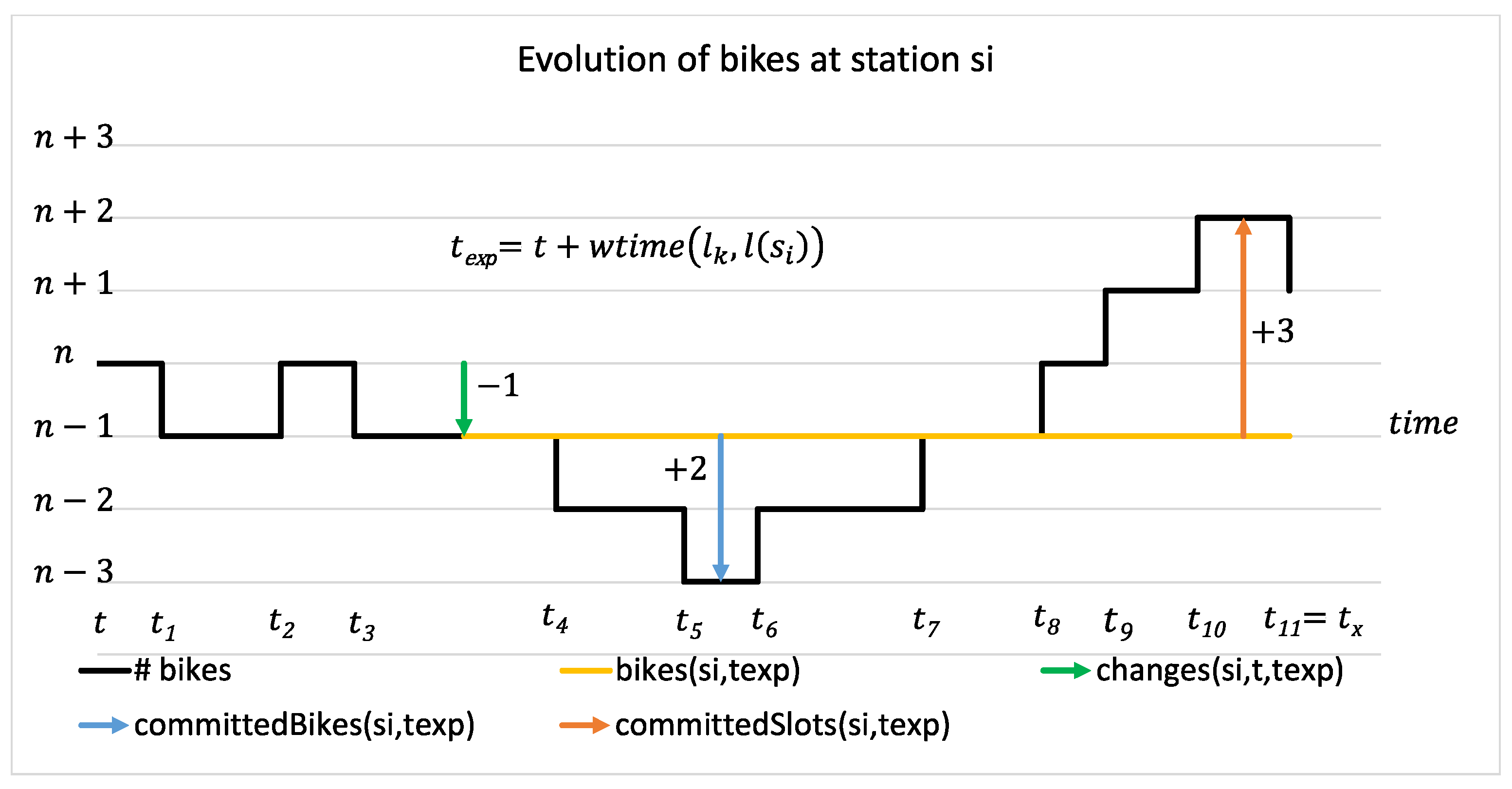
Figure 1 explains this idea in more detail. Suppose that at time
, user
(at location
) asks for a station to rent a bike, and the given option would be station
. At time
, there are
available bikes at station
, and the system tries to estimate the available bikes at the moment when
would actually arrive at
, i.e., at time
. Before instant
, the system has already recommended station
to other users for either renting or returning bikes, and assumes that those users will actually follow the recommendations and, thus, will return or take bikes at their expected arrival times. These actions are reflected in
Figure 1: at time
, a bike is expected to be taken; at
, a bike is expected to be returned, and so on. Let
denote the sum of the expected changes in the number of available bikes at station
in the time interval between the time of issuing a user request
and the potential arrival of the user at
. Here, each bike rental in this period counts as −1, and each bike return counts as +1. In the example,
would be −1. We can now estimate the number of bikes or slots expected to be available at the arrival time
of user
by
and
.
The system may also take into account the possibility that even if there are some bikes or slots available when user
arrives, some of those may have been already “committed”, e.g., they have been the basis for recommendations to other users who will eventually arrive after the expected arrival time of user
. In
Figure 1, this refers to the events at
,
, …
. Such events could be conceived as “implicit reservations”, and the system could try to “block” a number of bikes or slots for further recommendations. Here, we do not refer to a real blocking of a bike or slot for future users. Instead, the system would simply factor in this information when determining recommendations.
The number of “committed” bikes or slots depends on the sequence of expected events, and corresponds to the worst cases: the maximum and minimum values of
the expected changes after the user arrives, up to the last known event at time
(or
, if there is none). We denote these two values by:
and:
In
Figure 1,
signifies that three extra slots have to be “reserved” because a sequence of two taken and five returned bikes reaches a peak of 3 before
. On the other hand,
indicates that, at some point (in this case at
), two extra bikes will be taken from the station.
Taking into account the changes expected to occur at a station
after
and before the expected arrival of user
, as well as the “committed” bikes and slots, the estimated available bikes and slots at station
for a rental and a return request
and
are defined as:
where
is the estimated expected arrival time of user
at
.
With these definitions, we can define the
DistanceExpectedResources strategy as follows:
where:
where:
4.3. Expected Cost
It seems obvious that a better estimation of the available bikes or slots at the time of a user’s arrival at a station would prevent unsuccessful rental or return attempts. One way to achieve this is by estimating the probability distributions of available bikes at a station at a future instance in time, based on known demand patterns. In the following section, we describe how demands can be estimated, how we estimate the probabilities of finding an available bike/slot at a station at any time in the future, and how we use such probabilities to rank stations increasingly based on cost, combining the probability of finding a bike/slot and the expected time to reach a station.
Table 2 summarises the symbols and functions introduced in this section.
4.3.1. Demand Estimation
The demand for bike rentals and returns at a given station can be estimated from historical data and for different time intervals, days, weather conditions, etc. Supposing that such data are available, we use and to reflect the number of expected rental and return attempts at station during the time interval between and (. Given sufficient historical data, the calculation of these values is straightforward and, as such, we omit it here.
4.3.2. Probability Calculation
Using queueing theory, a station for renting bikes can be modelled as an M/M/1/K queue (see, e.g., [
21,
31,
35]. We consider that bikes arrive at a station and request the “service” to be rented. The arrival process (e.g., the return of bikes through users) and the “service” process (e.g., the rental of bikes by users) follow a Poisson distribution. The number of service channels is 1 and the maximum number of bikes waiting to be rented is K (the capacity of the station). The M/M/1/K queue is a special case of a birth–death process and of continuous-time Markov chains with K+1 states. Let
be the average bike arrival rate and
the average bike rental rate; given a station
, let
denote the (transient) state probability distribution and
the probability that the system is in state
at time
—that is,
represents the probability that there are
available bikes at station
at time
.
The time-dependent behaviour of the probability distribution can be determined by the system of differential equations (known as the forward Kolmogorov equations):
Given an initial distribution with , the system can be solved, obtaining the distribution at time t. Solving Equation (1) is mathematically complex, but an acceptable approximation can be found. In particular, in our experimental implementation, we use the fourth-order Runge–Kutta method for iteratively approximating solutions of differential equations (given an initial problem defined by , and , solutions for are approximated by iteratively calculating based on and . Taking small steps < , this process is repeated for steps, until is approximately . In this case, approximates ).
Let be a user rental request, a potential station, and the expected arrival time of user at station . Then, Equations (13)–(15) can be used to calculate the probability that would find an available bike (or slot) at station when they arrive at time These probabilities are denoted as and , respectively.
We define
the current probability distribution of (available) bikes locked at station
and the current time
, by:
Note that, similarly to the DistanceExpectedResources strategy defined before, we include changes in the number of available bikes at the station that are expected to take place between and . In particular, we approach such changes as if they had already been “blocked” at the moment of the user request (.
Using
as described above, setting
and
, and solving the system in the sense of Equations (13)–(15), we can approximate a solution for the probability distribution of available bikes at the time when the user arrives at the station
; meanwhile,
can be used to calculate the probability that user
will find a bike when they arrive at station
(at expected arrival time
):
As defined previously, represents the maximum number of bikes that are “committed”, e.g., that should be “blocked” for other users already known to arrive at station Thus, is not just the probability that a given user will find an available bike at a station when they arrive, but the probability of having enough bikes for the user as well as all other users who have been recommended to rent a bike at this station and are expected to arrive after user . For instance, if there are a maximum of two “committed” bikes, would be the probability that the number of available bikes at the expected arrival time is three or more.
In a similar way, in the case of a return request
, we must estimate the probability that, at the expected arrival time
, there is at least one slot available, plus the maximum required number of “committed” slots for future expected users. Considering the capacity of a station (
), the probability of having at least
slots is equivalent to having at most
locked bikes. Thus, we calculate the return probability by:
4.3.3. Expected Cost Recommendation
We combine distance and bike or slot probabilities to define the (local) rental or return cost of a station
for a user
:
and are parameters that represent the associated cost of getting to a station and finding no available bike or slot, respectively. In order to avoid distortions, in case we set It should also be noted that in the return cost we take into account not only the walking time from the station to the final destination, but also the cycling time to the selected station.
Using the cost functions, the definition of the
ExpectedCost recommendation strategy simply orders stations by increasing cost:
where:
where:
5. Evaluation of User-Centred Recommendation
We used the Bike3S simulation tool [
37] to validate the proposed strategies and compare their performance to the standard strategies. Bike3S is intended to evaluate different rebalancing strategies. The simulated infrastructure includes the location, capacity, and available bikes for each station. During a simulation, users are generated and interact with the infrastructure to rent or return bikes. They may ask a service (strategy) for a recommendation to choose their target station. Several user models can be defined and used in the same simulation run. Users’ appearance time, initial location, and destination are loaded into the simulator. A tool facilitates the creation of this information randomly. Different strategies can be implemented and easily integrated into Bike3S.
We replicated the operation of the BiciMAD public bike-sharing system in Madrid (Spain). This system covers an area of approximately 5 × 5 km of central Madrid, and is continuously growing. Currently it utilises ~200 stations and 2500 bicycles. The capacity of the stations is between 12 and 30 (most stations have 24 slots).
5.1. Simulation Experiment Setup
There are publicly available data on the usage of the BiciMAD system, in particular:
Data on the trips: Including, for each trip, the time of taking a bike, origin station, destination station, travel time, and approximate route. However, in order to anonymize the data, only the day and hour of the pick-up time of each trip are given (without minutes). Each trip includes a user type, with possible values representing regular or occasional users, BiciMAD staff, or unidentifiable users;
Situation of the stations: including the number of available bikes and slots, and whether or not a station was active.
In order to replicate a real-world scenario, we extracted the user data for a 24-h period (in particular, from 7:00 on 20 July 2018 to 7:00 on 21 July 2018). That period comprised 12,296 real user trips, whose data were used to generate the artificial users of our simulation. These data, however, only include the stations where a user took or returned a bike, but not their origin or destination location. Therefore, and in order to reflect the real situation as accurately as possible, we generated random origin and destination locations in an area spanned by a circle of 300 m around the rental station and the return station, respectively. Finally, the instant of creation of the simulated user was generated randomly within the hour of their appearance in the real-world data (with a uniform distribution), since the exact minute and second of appearance were unknown.
For specifying the initial station configuration in the simulated scenario, we used the official (real) data at the initial time (20 July 2018 at 7:00), at which there were 169 active stations with a total capacity of 4086 slots and 1792 bikes plugged in. However, since we wanted to analyse the performance of the different recommendation strategies in rather critical situations (where it is more likely to have empty and full stations), we reduced the station capacities and the number of plugged-in bikes at each station to approximately half of the original values—that is, in our experiments, we used 169 stations with a total capacity of 1995 slots and 896 bikes.
Even though the Bike3S tool can simulate the movements of people walking or cycling on real networks of roads and footpaths (using OpenStreetMap data), in our simulation, we used straight-line movements on the geographical map. The impact of this choice on the performance comparison of the analysed strategies was marginal, but it allowed us to reduce the simulation time considerably. We considered a default walking and cycling velocity of 1.4 m/s and 4 m/s, respectively [
38,
39]. However, since we used straight-line movements, and in order to adjust to more realistic values, we applied a velocity factor of 0.614. This factor was established based on comparing real and straight-line travel times between a set of origin/destination locations in Madrid (using OpenStreetMap data). Thus, the actual applied velocities were 0.8596 m/s for walking and 2.456 m/s for cycling. These velocities were used to simulate the movements of users; they were also used in the recommendation strategies to estimate the expected arrival times of users.
Using the specified setup, we carried out experiments to compare the performance of the five previously defined recommendation strategies:
ShortestDistance (SD);
InformedShortestDistance (ISD);
DistanceResources (DR);
DistanceExpectedResources (DER);
ExpectedCost (EC(x,y)), where and .
The user behaviour for renting a bike in the simulations was as follows:
A user appears at a geographical location at time and asks the recommendation system for a rental recommendation (with request ). The maximum acceptable distance in the experiments is set to m;
The recommendation system applies its strategy and returns a ranking of possible stations;
Given the ranking, the user filters out all stations that they have already tried. If no stations are left, the user will abandon the system without renting a bike. Otherwise, they walk towards the first station in the list of recommendations in order to rent a bike;
In case the user gets to a station and there are no available bikes, they repeat the whole process until they either abandon the search or finally find a bike. In this case, the value of the maximum acceptable distance () is reduced by the distance the user has walked already.
With this behaviour, a user will effectively abandon the system if they do not find any bikes within m.
For finding a return station, the process is as follows:
In the moment a user has rented a bike at a station , they issue a return request , where and are the current position and time, and is their final destination location;
The recommendation system returns a ranking of stations for returning the bike;
Given the ranking, the user filters out any stations that they have already tried, and selects the first remaining station for returning the bike;
In case the user gets to a station and there are no available slots, they repeat the whole process until they finally find a station to leave the bike (there is no possibility to abandon the attempt).
5.2. Simulation Results
The main aim of the recommendation strategies is to allow an efficient usage of a BSS in terms of the time the users spend to go from their origin location to their destination, as well as the unsuccessful rental and return attempts.
Table 3 compares the performance of the different user-centred recommendation strategies. The measurements we present are the following:
#a: number of users who dropped out (abandoned) the system, and percentage with regards to users that finished;
#fh: number of failed user rental attempts and percentage over all user rental attempts;
#fr: number of failed user return attempts and percentage over all user return attempts;
tt: average total time of users in the system; this is based on the time a user requires to go from their origin to a bike rental station, to cycle from there to a station to return the bike and, finally, to walk to their final destination. The value is averaged over all users who were able to rent a bike (i.e., who did not abandon the attempt);
AET: average station empty time; this is the time for which a station has been empty (without available bikes) and, thus, would potentially have been denying service. The value is the average over all 169 stations for the whole simulation period.
The first row of
Table 3 specifies a hypothetical optimal situation, where every user can obtain a bike at the station closest to their origin and return it at the station closest to their destination (i.e., the station capacities for rental and return are assumed to be unlimited). In this case, the average travel time would be 19.21 min. This travel time can obviously not be obtained in a real scenario.
Analysing the standard strategies (the first four strategies in
Table 3), there are different conclusions:
SD has the worst behaviour. Here, users go to the closest station, and many users will abandon their search because there are no bikes available. Furthermore, the travel time is quite high, because after an unsuccessful rental or return attempt, users may try at other stations and, thus, increase the time that they spend in the system. In comparison, ISD has a much better performance, because the probability of finding an available bike or slot is much higher if a user only goes to the stations that have available resources at the moment of the recommendation request.
DR combines the distance and availability of resources. In this way, it obtains a better dropout rate and, at the same time, a shorter travel time than SD and ISD. It should also be noted that, here, users would slightly prefer to rent/return bikes where there are more bikes or slots (within closed stations). This means, here, users implicitly improve the distribution of the bikes (and slots) among the stations. This can be seen in the reduction of the average empty time of stations.
The DistanceExpectedResources strategy (DER) clearly outperforms the standard strategies. Compared to DR, DER not only includes the bikes/slots in the analysis of appropriate stations that are available at the precise moment when a user issues a recommendation request, but also the expected changes up to the expected arrival of the user. In this case, the dropout rate can be reduced from 3.76% to 1.98%, whereas the average travel time remains nearly the same (21.62 versus 21.54 min). It should be noted that, with DER, the failed rental and return attempts are both 0. This is because with the specified experimental setting, the estimation of available bikes/slots is exact because (1) users always go to the recommended stations, and (2) the estimated travel time of users is the same as their actual travel time. In a real scenario, the benefit of DER with respect to DR should be somewhat smaller.
The last four rows in
Table 3 correspond to different instances of the
ExpectedCost strategy (
EC), which prioritises stations with a lower cost, calculated based on travel time and the (demand-dependent) probability of finding a bike/slot at the expected time of arrival of the user. This strategy’s performance varies for different values of
and
. In general, higher penalizations produce a lower abandonment rate, but increase the travel time. With
, for example, the abandonment rate is reduced to 1.21%, but the travel time increases to 23.21 min, which is considerable. A rather high value for
and low value for
obtains a good compromise. In this sense, for
and
both dropout rate and travel time can be slightly reduced with regard to
DER. With rather low penalizations, the abandonment rate is higher, but the travel time can be reduced, as with
EC (
1000,
2000).
In
Figure 2,
Figure 3 and
Figure 4, we analyse the behaviour of
EC with varying values for
and
.
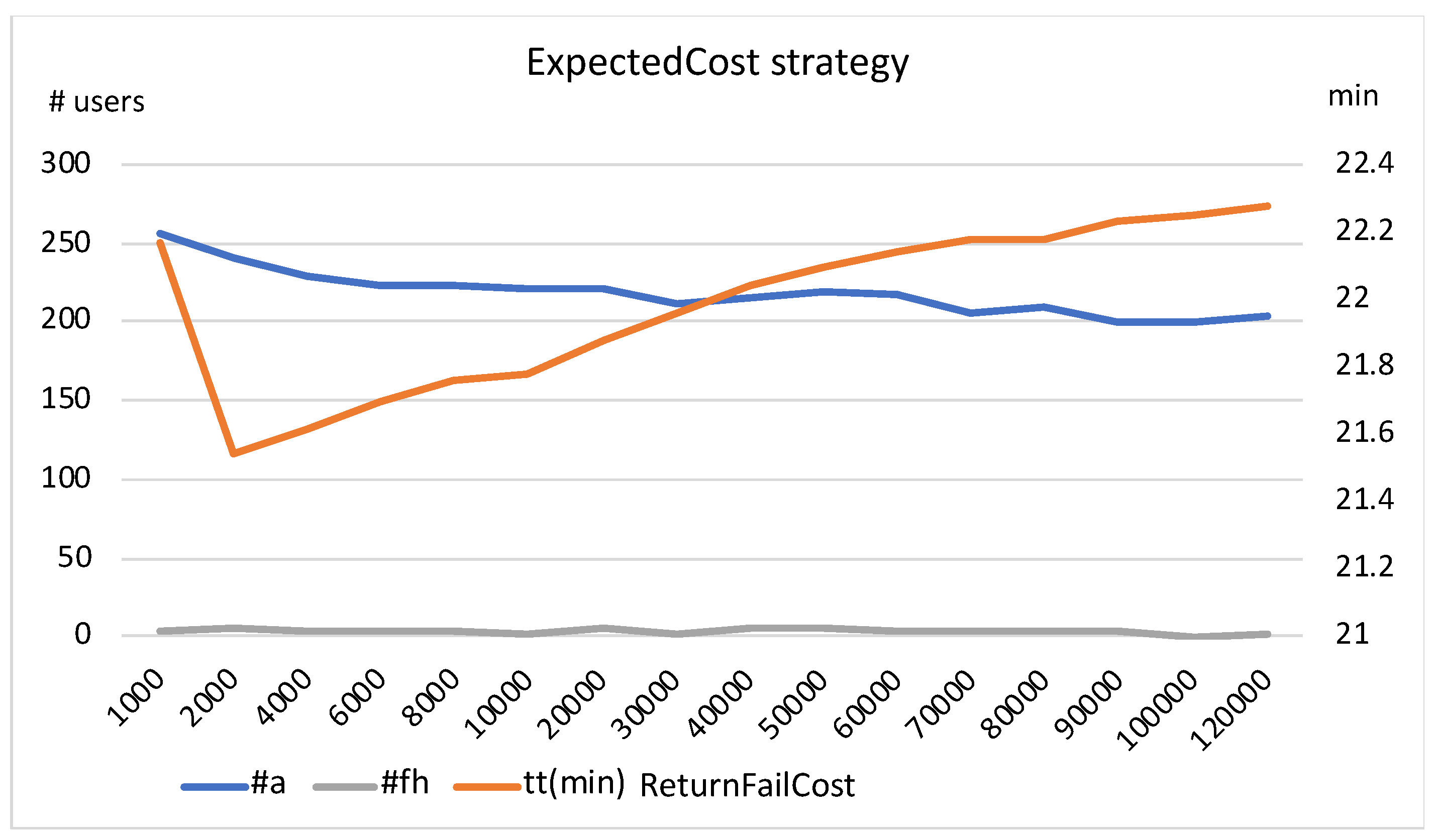
As shown in
Figure 2, the abandonment rate decreases with increasing
, and the travel time decreases up to a value of ~2000, and then increases. At higher values, both travel time and abandonment rate become almost stable. The lowest travel time is obtained with a value of ~2000. Exactly the same behaviour is observed for other values of
. We also observed in our experiments that, as the value of
increases, the number of failed returns (#fr) falls rapidly towards ~0 at the value of
= 4000 (for the sake of clarity, this is not shown in the figure).
In
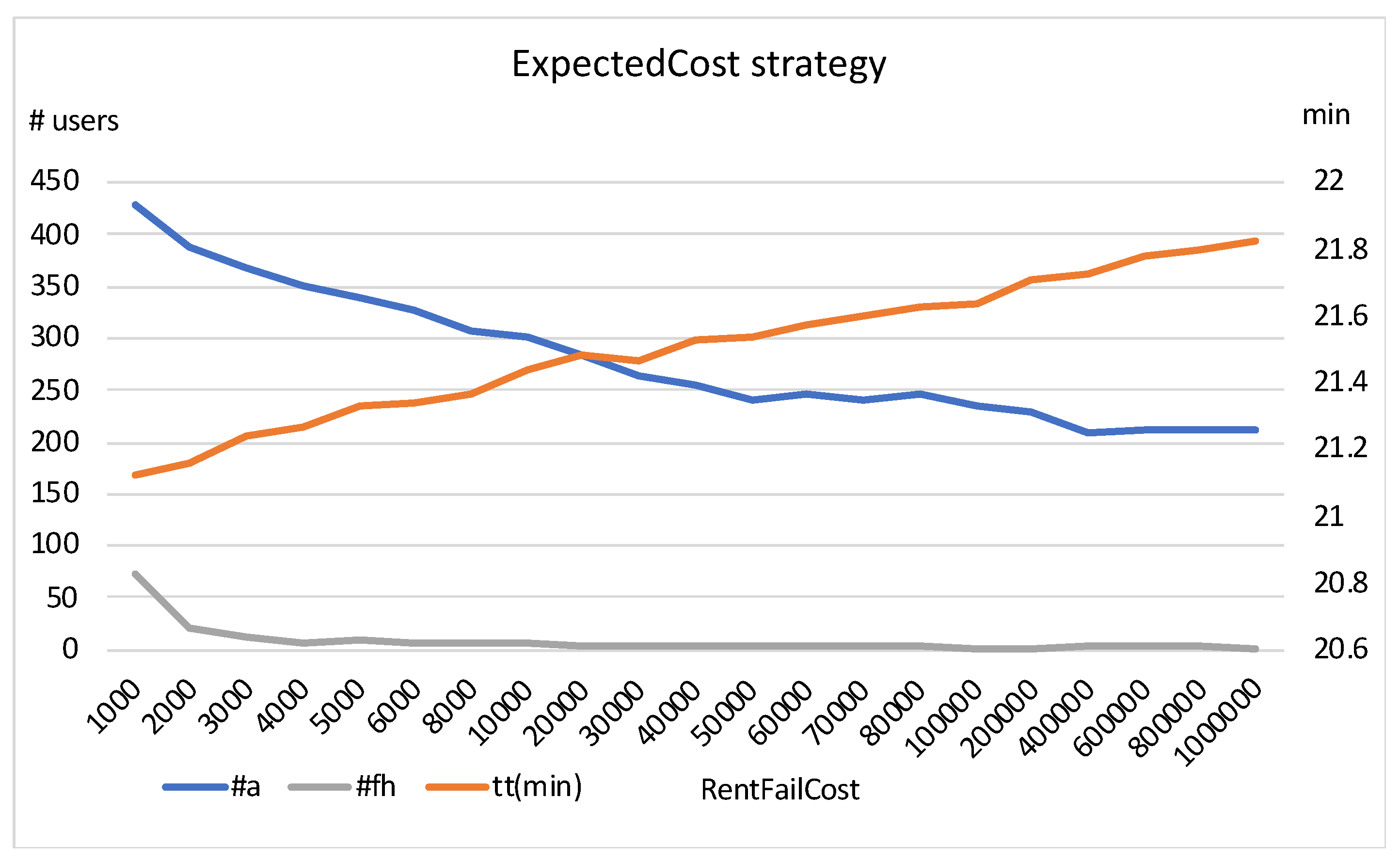
Figure 3, we show a fixed value of
(the value that generally obtains the lowest travel time for different values of
), and we increase
. As can be seen, higher values of
produce lower abandonment rates and fewer failed rental attempts, but lead to increased travel times. It seems that the values remain almost stable at a certain point.
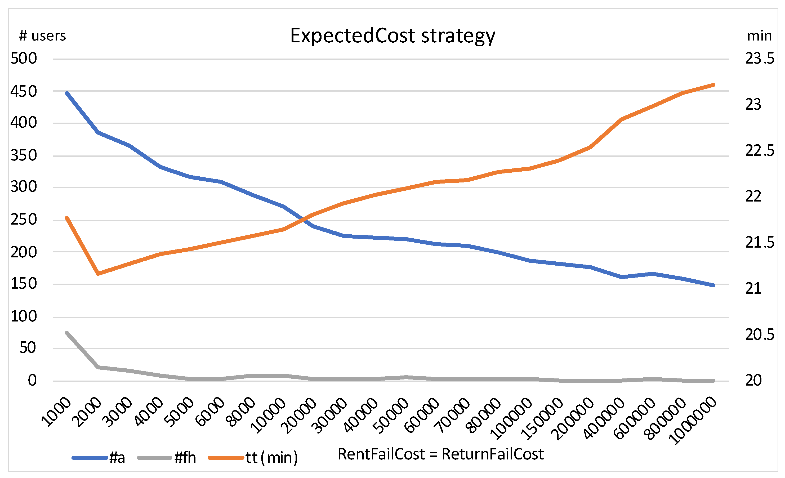
If we increase
and
at the same time, as shown in
Figure 4, the abandonment rate reduces continuously and considerably, but at the cost of an increase in travel time. The failed rental attempts tend towards 0.
Comparing the ExpectedCost strategy with DistanceExpectedResources, the former can be parametrised in order to prioritise abandonment rate or travel time. However, it is interesting to observe that for the same ratio of travel time, both methods obtain almost the same dropout rate, and vice versa. In other words, the rather simple DER strategy performs as well as the much more sophisticated EC strategy. In our opinion, the explanation of this fact is that the DER strategy not only proposes an appropriate station to rent or return a bike in terms of the utility for an individual user, but also encourages users to take or return bikes at stations with more bikes/slots. In this way, the strategy implicitly improves the unbalancing problem, helping to obtain a better distribution of bikes (and slots) and, thus, to reduce the abandonment rate and the travel time of potential future users.
6. Recommendation Based on Local and Global Utility
As argued previously, the DER strategy with a rather simple calculation model has a quite acceptable performance, because it combines the local utility of a recommendation for a user with a certain improvement of the global situation for the future. In this section, we use this idea to extend the ExpectedCost strategy in the same sense. The idea is to account not only for the cost of a station for a certain user, but also for the changes in the costs to potential future users, if they decide to take (or return) a bike at given station. In particular, taking into account the future demand of bikes or slots at a station, we estimate how taking or returning a bike will increase or decrease the number of expected unsuccessful rental and return attempts of future users at a station within a certain timeframe.
6.1. Calculating the Future Impact of Rentals and Returns
To estimate the impact that a bike rental or return has globally on system performance, we analysed how such an event would change the number of expected unsuccessful rental and return attempts of future users—that is, the impact can be measured through the difference in expected unsuccessful events during a given time interval if a bike is taken (or returned) at the beginning of this time interval. Moreover, given a station and the expected rental rate during the interval (obtained by analysing historical demands, for example), the number of expected unsuccessful rental attempts is the number of all rental attempts multiplied by the probability that such attempts fail. We formalize this idea below.
Modelling a station
as a queue, the average probability of the station being in state 0—that is, having no available bikes—during a time interval
with
is given by:
Based on the system of differential Equations (13)–(15), and given the initial probability distribution
and a step-size
with
, we can use the fourth-order Runge–Kutta method (RK4) to estimate
. Let
, where
, denote the sequence of iteratively calculated values for
from
to
at steps
with RK4. Then, we can use a Riemann sum to approximate
:
Finally, given the rental appearance rate for a station
in the interval
,
, the expected number of failed rental attempts in the interval is estimated by:
In a similar way, we can calculate the expected failed return attempts for a station
in an interval
:
where
is the capacity of station
.
If a user
issues a rental request
, we use
and
to estimate the future impact that a potential rental would have at a station
. The idea is to first calculate the probability distribution of available bikes when the user arrives at the station. Afterwards, we analyse the expected rental and return failures that would arise after the arrival and during a given timeframe (
) if the user rented out a bike and if they did not do so. The difference between these values can be used as a measure for estimating the future impact of renting a bike at a station. Formally, we first calculate the probability distribution of bike availability at the expected arrival time of user
, with
, as explained in
Section 4. Using
as the initial distribution, and applying Equations (24)–(26), we can calculate
and
Then, we transform from
to a distribution
, where one bike is “taken” away. This means:
Now, taking
as the initial distribution, we calculate
and
. Finally, we can obtain the rental failure impact (
) and return failure impact (
) of the potential rental:
It should be noted that , because the expected rental failure rate is necessarily higher if a bike is taken from a station; thus, would be positive. On the other hand, , since the number of available slots increases if a bike is taken from the station. Thus, the values of and represent the expectation of failed rental and return attempts that are caused by user when they take a bike at station .
In a similar way—but transforming
to a distribution
, where one bike is “added”—we can calculate the expected failed rental and return attempts that are caused if user
returns a bike at station
:
6.2. Recommendation Based on Expected Cost and Future Impact
We calculate the global cost of renting at a station by combing its local cost with the impact on the overall system in the next given timeframe:
is a parameter that assigns more or less importance to the local cost versus the global impact.
and
represent the cost associated with the number of extra future rental and return failures, respectively. This cost should depend on whether a potential user who arrives at a station and fails to rent or to return a bike has some alternative to rent or return a bike at a station nearby. With this idea, we define:
where
and
. This means that
is the lowest local cost of stations in the vicinity of station
(within a distance of
meters), and taking the parameter
as the penalization cost. In the worst case—e.g., when no station exists within a distance of
meters from
—the value of
will be
. In the same way,
will be at most
. Note that the local costs for users who would arrive at station
are appproximated by considering they arrive at mid timeframe after the arrival of user
.
Based on the global costs, we define the recommendation strategy
ExpectedCostFutureImpact:
where:
where:
In summary, the parameters of this strategy are:
—the maximum distance to rental stations;
and —the penalization costs applied if a user is unsuccessful when trying to rent or return a bike;
—the timeframe for predicting the future impact of a rental or return action;
and —the penalization costs applied when estimating the costs of local alternative stations for users who cannot find a bike or slot at station in the future;
—the maximum distance to consider alternative stations for users who cannot find a bike or slot at station ;
—the factor applied to the global impact on the cost estimation.
7. Evaluation of ExpectedCostFutureImpact Recommendation
We used the same settings as in
Section 5 to evaluate the
ExpectedCostFutureImpact strategy. In the experiments, we fixed the following parameters: the values of
600 m, as a reasonable distance that a user might be willing to walk to get a bike, and
500 m.
In the first set of experiments, we analysed this approach with different penalization costs, where the timeframe
was set to 1 h and the factor
= 1. Some results are presented in
Table 4.
Analysing the results presented in the table, we can observe that, in general, higher penalization costs lead to lower dropout rates but longer travel times, whereas lower costs have the opposite effect: more abandonments and shorter travel times. A good combination of both metrics can be obtained with values close to the following:
= 3000,
= 2500,
= 3000, and
= 1000. In particular, the abandonment rate can be reduced considerably if a recommendation considers not only the local cost for a user (to rent or return a bike), but also the impact on potential users in the future. For example, the strategy with the penalization schema 3000/2500/3000/1000, as compared to
EC (
70,000/
2000), reduces the number of abandonments from 240 to 15 by maintaining the same travel time (21.6 min). In
Section 5, the
EC (
70,000/
2000) strategy showed a good behaviour in terms of abandonment rate and low travel time.
Using the penalization cost pattern 3000/2500/3000/1000, and fixing the factor
= 1, in
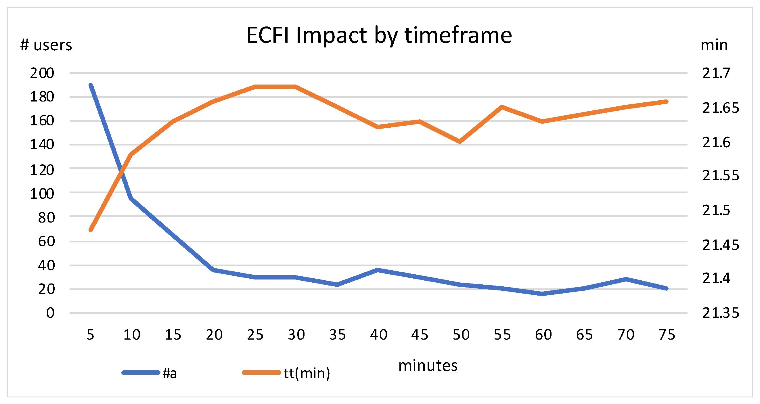
Figure 5 we analyse the influence of the prediction timeframe in the results.
Figure 5 indicates that, as expected, short prediction timeframes present higher abandonment rates but faster travel times. It is more likely that future users will not find an available bike or slot, but users are sent to “closer” stations since the considered future impact will be lower. At some point, the values for dropout rate and travel time tend to stabilize, and even increase slightly. Good results are obtained with a prediction timeframe of ~20 min.
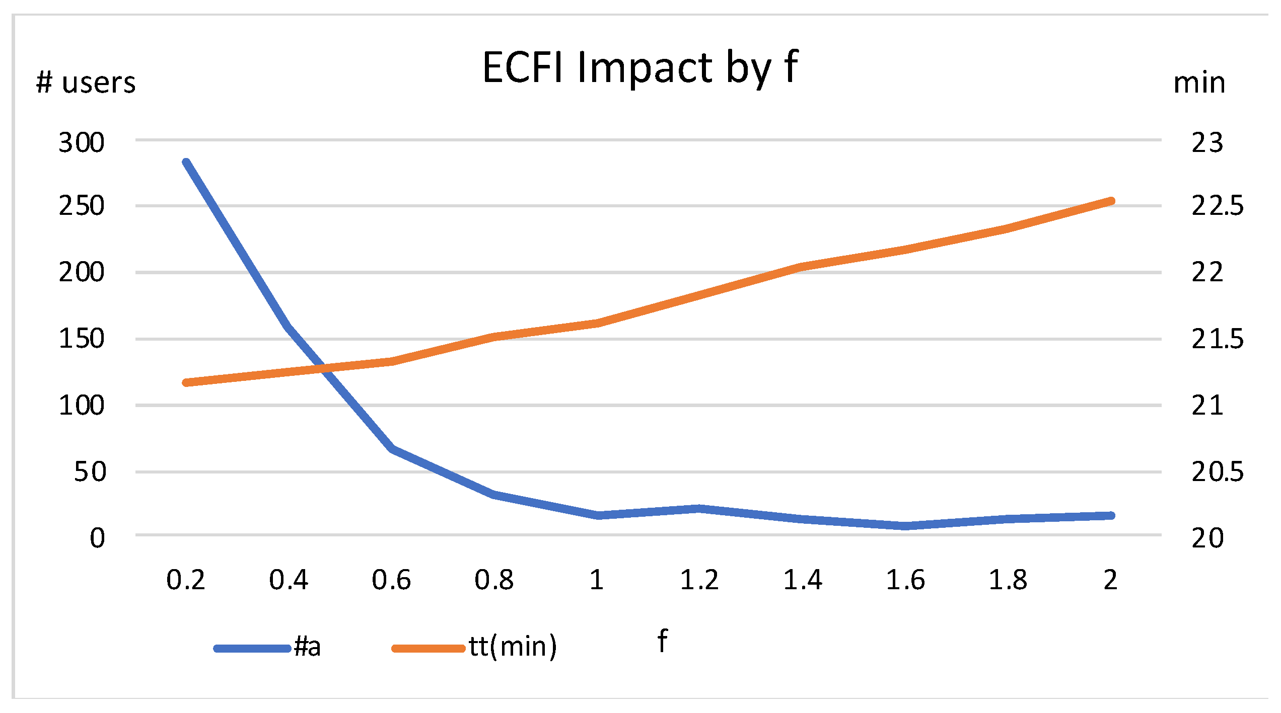
The best way to prioritise between average travel time and abandonment rate is via the factor
. In
Figure 6, we show different results obtained when varying
. Low values for
decrease travel time, but lead to more abandonments. A good compromise is obtained with
around 1.
As we mentioned in
Section 5, the experiments in this paper are based on real data, but we reduced the station capacities and the overall number of bikes in the system to approximately half of their original values. The reason for this was that such a situation is more challenging and, thus, the differences in the recommendation strategies are more appreciable. In
Table 5, however, we present and compare the standard strategies with the best variations of the
ExpectedCost and the
ExpectedCostFutureImpact strategies, in a scenario with the original (real) station capacities and bike numbers. As expected, all strategies significantly improved their performance with real station capacities. As shown, the novel strategy
ExpectedCostFutureImpact proposed in this paper also performs better than the other strategies in this situation, in terms of both abandonment rate and travel time.
8. Conclusions
Bike-sharing systems are becoming an integral part of intelligent transportation infrastructure in smart cities. Station-based BSSs have the advantage of being more resilient with regards to misuse and vandalism, and also account for seamless charging if the BSS fleet contains electric bicycles. A typical problem in station-based BSSs is the possibility that some stations may run out of available resources due to high and unbalanced demands at peak times. However, if no bikes are available near their location, or if finding an available parking slot at the destination is difficult, users may drop out of the BSS and use other, less eco-friendly means of transportation.
In this paper, we addressed the balancing problem in BSSs by developing recommendation strategies that help users to select a station to rent or return a bike, considering the distance/time to that station as well as the likelihood that they will find a bike/slot when they actually arrive at the station.
Our contribution is twofold: In the first part of the paper, we presented and analysed station selection (or recommendation) strategies that are user-centred—that is, they try to find the best station considering only the utility or expected cost of a specific user. We presented the DistanceExpectedResources strategy, which assumes that recent recommendations are being followed by users and, thus, can better estimate the resources that are expected to be available at the moment when a user actually arrives at a certain station. We also presented the ExpectedCost strategy, which minimizes a user’s cost, combining the distance from their origin (or destination) to the location of candidate stations, and the probability of finding an available bike (or empty slot) when they arrive. This strategy models stations as queues and uses demand data to estimate the probability of finding available bikes or slots. We compared the performance of the presented strategies through simulation experiments with real data from the BiciMAD BSS in Madrid. Both methods outperform baseline station selection strategies such as “going to the closest” or “going to the closest station with available bikes/slots”, in terms of both (1) the number of users who abandon the system without renting a bike, and (2) the total time in the system.
In the second part of the paper, we proposed a station recommendation strategy that seeks an equilibrium between local (user-centred) and global utility. With regard to the latter, recommendations prioritise stations that are good for a particular user, but also imply some positive impact on the distribution of bikes and slots in the overall system, and for potential future users. In particular, we defined the ExpectedCostFutureImpact strategy, which extends the ExpectedCost approach by also analysing the impact that choosing a particular station will have on future rentals and returns. In the simulation experiments, this solution outperformed all other strategies, with respect to both the number of abandonments and total travel time.
In future works, we aim to look into explicit (e.g., monetary) incentive mechanisms so as to persuade individually rational users to follow our recommendations while maintaining their trust in the system. These incentives are likely to be proportional in some way to the globalRentCost. Another interesting line for future research in this context consists of learning, from experience, the likelihood that specific (types of) users will follow the recommendations given. This would allow a more fine-grained adjustment of our recommendation model based on user profiles, and could also be used to implement specific user-centred incentives. Finally, as we mentioned in the introduction, BSSs could be conceived as part of a sophisticated multimodal intelligent transportation solution. The synergic effects within such a system of systems open up a whole range of new opportunities, especially with regards to better availability of green transportation services and a reduced number of dropouts.


