Abstract
This study focuses on the acoustic installation effects that may occur during typical aeroacoustic experiments when the latter are conducted in a closed-vein wind tunnel. More precisely, in regard to the specific problem of airfoil trailing edge noise, an analytical model is derived, which allows predicting the wall-induced reverberation effects that such a noise shall be subjected to, when radiating within a closed-vein, hard-wall, wind tunnel. These effects are then assessed through a parametric investigation so as to characterize their impact on in situ acoustic measurements that would be performed using flush-mounted microphones located on the vein’s walls. From a phenomenological perspective, the study highlights how important the reverberation effects by the vein can be. In particular, results reveal how their impact on the noise measurements may greatly vary, depending on the trailing edge noise source location (i.e., the airfoil incidence) and, to a lesser extent, its frequency. The outcomes allow identifying these locations where the installation effects are least, i.e., where to better position a flush-mounted microphone, should in situ noise measurements be conducted. From a methodological viewpoint, the study showcases how the proposed formalism could constitute a simple albeit useful diagnosis tool for mitigating the experimental biases weighing on airfoil trailing edge noise tests to be conducted within closed-vein facilities, whether this would be done a priori by flush-mounting the microphone(s) where these biases are minimal or a posteriori by de-biasing the noise measurements accordingly.
1. Introduction
Industries across all sectors share a common need for innovative technologies offering both higher performance and lower emissions. Although chemical emissions are of primary importance, acoustic ones have become just as critical. Among the numerous sources of environmental noise, those of aerodynamic origin plague various industry sectors, e.g., transport (aircraft noise, railway noise), energy (wind turbine noise), and so on. One can more especially cite the so-called airfoil self-noise, which is generated when a streamlined profile (wing, blade, etc.) is immersed into an incoming flow. As the pioneering study by Brooks et al. [1]. revealed, airfoil self-noise is made of five primary components, most of which result in broadband and/or tonal noise emissions originating from the airfoil trailing edge (TE). For instance, the so-called laminar boundary layer TE (LBL-TE) noise [1,2,3] stems from the interaction of the airfoil with low to moderate Reynolds number flows, typically resulting in one to several tonal, dipolar, acoustic emissions of high intensity. The latter are believed to originate from an aeroacoustic feedback loop mechanism, which involves a selective amplification of laminar boundary layer instabilities due to the recirculation bubble(s) that may exist on either side of the airfoil when flow detachments occur (e.g., pre-stall onset) [2,3]. Other TE noise sources exist, such as the vortex shedding entailed by a blunted trailing edge (which also generates a strong tonal, dipolar acoustic emission), or the flow separation occurring in the early stage of stall (as opposed to the deep stall one, which rather results in noise radiating from the entire airfoil). Given its multiple components and complex physics, the airfoil trailing edge (TE) noise is still only partly understood [1,2,3], despite half a century of investigations using either experimental [1,4,5,6,7,8,9,10,11,12,13,14,15,16,17,18,19], theoretical [15,16,17,18,19], or computational [20,21,22,23,24,25] means.
Because in situ testing is extremely costly to perform, it is common to characterize aerodynamic noise emissions through small-scale experiments. Traditionally, aeroacoustic tests are conducted within anechoic, open jet wind tunnels, whereas closed-vein installations are rather devoted to pure aerodynamic experiments. Indeed, although closed-vein wind tunnels are known to restitute more accurately the actual flow physics, their confined character incur some unwanted acoustic installation effects, namely, noise reverberation and resonance phenomena due to acoustic backscattering on their walls. It is known, however, that open-jet facilities also come with their own issues, which may complicate (and, in some cases, jeopardize) the experimental characterization and subsequent physical analysis of aeroacoustic phenomena that are sought after. First, open-jet facilities are not entirely free from those side-effects that are commonly attributed to closed-vein wind tunnels, to begin with reverberation issues. Indeed, under some circumstance, the interaction of the noise sources with the experimental apparatus (e.g., mounting side-plates, nozzle, collector) may result in significant acoustic backscattering effects [8,13,20,26,27,28]. Alternatively, the interaction between the shear layers generated at the nozzle lips and the mock-up may incur some extraneous noise emission (as clearly pointed out by Moreau et al. [8] regarding the well-known airfoil noise experimental campaign by Brooks et al. [5]). Even more specific to airfoil noise tests is the fact that, when located within an open jet, a lifting body deflects more importantly the flow streamlines (downwash effect). This results in a modified flow incidence (e.g., effective angle of attack) whose uncertainty can be of several degrees between different apparatus [8,13]. This is likely to alter the airfoil self-noise emission processes, especially for what concerns its TE noise component, which is known to be extremely sensitive to the incoming flow (overall loading, separation/recirculation bubble location, etc.). Aside from that, the flow quality may also be altered by other phenomena, such as low-frequency pressure fluctuations (or “pumping” effects), which are inherent to open-jet wind tunnels. Last but not least, open jets are likely to alter the far-field noise radiation, due to both acoustic refraction (by the jet shear layers [28]) and acoustic diffusion (by the jet fine scale turbulence). Although these effects can be corrected a posteriori through analytical and/or semi-empirical means [29,30,31,32,33], such corrections imply some restrictive assumptions that make them partly conclusive only [25] (e.g., the plug flow model by Amiet [29,30]).
All these reasons explain why some researchers explored the use of closed-vein wind tunnels for conducting aeroacoustics experiments [34], including several studies focusing specifically on airfoil TE noise [6,7,9,10,11,12,13,14]. Following that, the model is placed within a closed-vein test section whose walls are then equipped with flush-mounted microphones so as to measure the noise signature. The latter is expected to be closer to what happens in reality, since the closed-vein ensures a flow that is similar to those obtained in real conditions (as well as in computations). Only the confinement effects need to be handled, whether they relate to aerodynamics (blockage effects) or acoustics (reverberation effects). Concerning blockage effects, they are not deemed to be too problematic, since airfoil TE noise experiments are usually performed for reduced values of flow speed and/or incidence [1]. For instance, the LBL-TE noise is known to primarily emerge at low to moderate Reynolds numbers, which implies a small airfoil chord and/or a low flow speed. In addition, it is also known that LBL-TE noise is generated when the flow is laminar over most of the airfoil’ surface, which requires the incidence to be kept small enough, namely, below the stall angle. All in all, one can thus expect blockage effects to be rather minimal for an airfoil TE noise experiment that would be conducted in a closed-vein wind tunnel. Regarding reverberation effects, one option is to cover the test section hard-walls with noise absorbing materials [6,11] or to replace them with as-like anechoic panels (Kevlar) [12,13]. This, however, requires to re-design part of the wind tunnel, which may raise practical challenges - from simply modifying its walls up to surrounding it by an anechoic environment. Furthermore, this also raises fundamental questions, e.g., how to properly design acoustic liners and/or deal with their potential issues [35] when the latter are to be exposed to grazing flows, how to mitigate the relative flow alteration [13], acoustic transmission losses [13] and/or background noise exacerbation [36] incurred by Kevlar panels, etc.
Another, simpler, option would be to keep the hard-wall wind tunnel as is, while accounting properly for its reverberation effects. This, for instance, is commonly achieved when performing noise source localization using acoustic holography techniques within reverberant environments [37,38,39]. There, specific post-processing techniques are employed, which allow de-biasing the localization results from all reverberation effects induced by the vein. In the present case, such de-biasing could be achieved a posteriori by correcting the noise measurements from all reverberation biases, or they could rather be conducted a priori by flush-mounting the microphone(s) where these biases are less. This however requires the reverberation effects to be characterized, both qualitatively and quantitatively. As was previously shown by the present author and other researchers for similar airframe noise problems, assessing the so-called acoustic installation effects incurred by facility apparatus can be achieved using numerical simulation [20,27,28]. Doing so, however, usually entails a computational complexity and/or cost which may restrict the generality of the observations made, if only because it prevents extensive parametric investigations to be performed. Therefore, one may wish to rather privilege the use of analytical means, in the fashion of what was made for exploring the aerodynamic installation effects incurred by closed-vein wind tunnels [40,41]. To the author’s knowledge, assessing analytically their acoustic counterpart has not been attempted yet. This is what is proposed in the present study, whose outcomes are both methodological (modeling aspects) and phenomenological (acoustic installation effects). More precisely, here, an analytical model is first derived, which allows predicting the wall-induced reverberation effects that an as-like airfoil TE noise source (2D harmonic dipole) shall be subjected to, when radiating within a closed-vein, hard-wall, wind tunnel. These effects are then assessed through a parametric investigation so as to characterize their impact on noise measurements that would be performed using flush-mounted microphones located on the vein’s walls.
The paper is organized as follows; Section 2 details the derivation of the analytical model, whose relevance is then illustrated through a representative test case. In Section 3, the latter test case is generalized through a parametric study, which offers characterizing better the acoustic installation effects and their underlying physical mechanisms. Finally, some conclusions and perspectives are drawn.
2. Analytical Model
In the present section, an analytical model is derived, which allows predicting the installation effects incurred by the wind tunnel vein onto the TE noise emission. The derivation is initially kept as generic as possible, being then tailored to the present problem of a dipolar, tonal, source. It is then illustrated via a representative test case that would correspond to a typical airfoil TE noise experiment conducted within a closed-vein wind tunnel.
2.1. Problem Description
We consider the generic problem of an airfoil that is located within a closed-vein wind tunnel whereas being exposed to an incoming flow. Under those conditions the airfoil tailing edge (TE) is likely to generate acoustic waves, which then propagate within the duct. During their propagation, these noise waves are subjected to various acoustic installation effects coming from the environment, namely reflection by the vein walls, as well as convection and refraction by the flow. Let us assume that the flow is slow enough for its convection (and subsequent refraction) effects onto the acoustic propagation to be legitimately neglected. In this case, the installation effects reduce to the reflection by both the top and the bottom walls. In addition, under such a low Mach condition, the TE edge noise source mostly behaves like a 2D dipole [42,43], whose radiation axis is orthogonal to the airfoil centerline.
To model this, let us consider a 2D airfoil of chord c (c = a + b) that is located within a duct of height 2h (cf. Figure 1). The airfoil is set at an angle-of-attack α whereas being exposed to an incoming flow of axial velocity , with M the Mach number, and c0 the sound speed of the medium whose density is . Let us consider that the trailing edge, which is located at , emits acoustic waves within the duct.
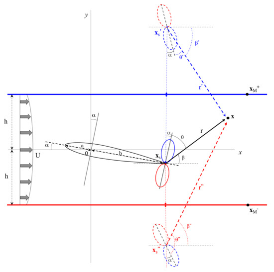
Figure 1.
Sketch of the experimental set-up, with geometrical construction of the specular reflections using source images.
2.2. Instantaneous Pressure
By the principle of superposition, the instantaneous acoustic pressure field perceived by any given observer can be defined as
where and stand for the incident and reflected pressure fields, respectively.
2.2.1. Incident Pressure Field
The incident pressure field results from the direct ‘source-to-observer’ propagation of the acoustic waves, and it can be expressed as follows:
where is the pressure resulting from the source emission alone, i.e., out of any installation effect due to the duct. In the (here assumed) absence of any flow, this incident pressure solely depends on both the propagation distance (r) and the emission angle (θ) between the source and the observer. The propagation distance is simply the Euclidean length between the two points, which in the present case of a two-dimensional (2D) problem, is given by
2.2.2. Reflected Pressure Fields
The reflected pressure field results from the specular reflection of the emitted acoustic waves by both the top and the bottom walls. Still using the principle of superposition, it can be expressed as
where and , respectively, stand for the reflected field originating from the top and the bottom wall alone. Each one of these reflected pressure fields can be constructed using a source image [39], i.e., a virtual source that would mirror the actual one through the considered wall (cf. Figure 1).
Of note, we here limit ourselves to primary reflections, i.e., we neglect all secondary reflections that would come from multiple and successive backscatters by the top and bottom walls (e.g., noise source → top (resp. bottom) wall → bottom (resp. top) wall → observer). Accounting for these additional reflections would imply considering an infinity of virtual sources, to be located one above the other (i.e., the second virtual source would correspond to the image of the first one, once mirrored by the opposite wall). Doing so would complexify the analysis unnecessarily, considering the less critical role played by these secondary sources. Indeed, compared to their primary counterparts, these further scattered waves are likely to see their amplitude decreasing rapidly, due to their comparatively longer propagation path. This, at least, is valid for observers that are located close enough to the actual source such that they experience a significant relative difference between the direct (actual) and the scattered (virtual) propagation distances. This would not hold for observers located further away from the trailing edge (e.g., ), and for which secondary reflections should be kept.
Pressure Field Reflected by the Top Wall (Alone)
The pressure field reflected by the sole top wall corresponds to a virtual incident field that would be emitted by the source image (cf. Figure 1):
where and respectively stand for the virtual propagation distance and emission angle between the mirroring source and the observer (sketched in blue color in Figure 1). With such mirroring source located in , similarly to above, the virtual propagation distance becomes
By construction, the virtual emission angle is now given by
where
Notably, in the present case of a top wall that is parallel to the x-axis, one has
and
Therefore
and
Pressure Field Reflected by the Bottom Wall (Alone)
In a similar fashion, the pressure field reflected by the sole bottom wall corresponds to a virtual incident field that would be emitted by the source image (cf. Figure 1):
where and respectively stand for the virtual propagation distance and emission angle between the mirroring source and the observer (sketched in red color in Figure 1). Such mirroring source is now located in , and the virtual propagation distance thus becomes
Here again, the bottom wall is parallel to the x-axis, which leads to
and
Therefore
and
2.2.3. Total Pressure Field
In summary, the resulting pressure field at any given observer is given by
with
2.2.4. Incident, Reflected and Total Pressure Fields at the Wall
Let us consider the specific (albeit common) situation where in situ noise measurements are achieved using a flush-mounted microphone that is placed on one of the duct walls. In this case, the observer coordinates become . For an observer that would be placed on the top wall (i.e., ), the overall pressure field thus becomes
with
One can here notice that and , i.e., . Therefore, in this particular case, the acoustic field that is reflected by the top wall matches exactly the incident one. The latter will thus be doubled up by the former, due to perfectly correlated constructive interferences. On the other hand, the acoustic field that is reflected by the bottom wall will bring an additional modulation, through either constructive or destructive interferences.
For an observer that would be placed on the bottom wall , the pressure becomes
with
In this case, and , i.e., , that is, the acoustic field reflected by the bottom wall is the same as the incident one. Similar to what happens for its top wall counterpart, both fields will sum up, due to perfectly correlated constructive interferences. The result will then be further modulated due to the acoustic field that is reflected by the top wall, which will induce either constructive or destructive interferences.
2.2.5. Particular Case of a Harmonic Dipolar Source
Let us consider the particular albeit common situation where the TE noise source corresponds to a harmonic dipole pulsating with a frequency f. It emits acoustic waves that then propagate within the (supposedly quiescent) medium, being characterized by a wavenumber where is the source pulsation.
Incident Field
Under a far-field assumption (i.e., ), the resulting incident field can be approximated as follows:
In the above expression, stands for the amplitude whereas relates to the directivity, with the angle subtended by the observer to the dipole axis (cf. Figure 1). For a dipole under a far-field condition (compact source), the directivity is that of a cardioid, i.e., the acoustic radiation is maximum along the dipole axis, and nil in the orthogonal direction:
When the dipole corresponds to a point source of strength Q, it radiates in a 3D fashion, thereby emitting waves of maximum amplitude:
If, however, the dipole rather corresponds to a line of sources, it radiates in a 2D fashion, and the amplitude becomes:
This last case corresponds to the present problem, for which the airfoil trailing edge noise acts as a 2D dipole located at the TE. One can thus express the source field as follows:
Or, when equivalently expressed in non-complex quantities,
In the above, refers to the maximum amplitude, which is driven by the frequency (on which depends the source ‘compactness’, through the wavelength):
Reflected and Total Fields
In this particular case of a harmonic dipolar source, the reflected field becomes
with
and
The above reflected fields (Equations (46) and (47)) will sum up with the incident one (Equation (43)), thereby leading to the total pressure field.
Incident, Reflected and Total Pressure Fields at the Wall
For an observer located on the top wall, the resulting overall pressure is obtained by replacing the expression of Equation (32) with those appearing in Equations (43) and (47).
Similarly, for an observer located on the bottom wall, the resulting overall pressure is obtained from Equation (37) using expressions from Equations (43) and (46).
2.2.6. Illustration via a Test Case
To illustrate the above developments, let us consider a 2D test case that is representative of a typical airfoil TE noise experiment that would be conducted within a closed-vein facility of half-height h (cf. Figure 1). The airfoil has a chord and it is rotated around its mid-chord point () with an angle of attack α = 20°. Let us assume that, under those conditions, the airfoil emits a strong, tonal, dipolar TE noise emission of frequency corresponding to a Strouhal number (with the sound speed, m/s). In real life, this test case could correspond to a small-scale experiment for which a 10 cm chord airfoil would be blown within a vein of height 2h = 0.5 m, thereby radiating a TE self-noise of frequency f = 1 kHz (which is consistent with typical observations from the literature).
Notably, since the wavenumber can be expressed as a function of the Strouhal (), the far-field condition invoked in the dipole approximation ( cf. Section 2.2.5) translates into . In the present case (St = 0.294), this condition is verified for all observers such that .
Figure 2 depicts the instantaneous pressure field corresponding to an emission time of 10 periods (t = 10T), with such field being decomposed into several components, for illustration purposes. First, the incident field clearly reveals how the TE dipolar source emits following a very directive fashion, with radiation lobes that are oriented orthogonally to the α-inclined airfoil center line (see Figure 2a). This incident field is then reflected by the top wall, leading to backscatter patterns which resemble to the radiation of a virtual source that would mirror the real one (see Figure 2b). Such reflected field finally sums up with its bottom wall counterpart, thereby leading to the strong interference patterns that translate the vein’s installation effects (see Figure 2c). Once cumulated, these various components lead to the total pressure field (see Figure 2d), which differs significantly from the original one (compare for instance Figure 2d to Figure 2a).
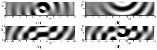
Figure 2.
Low frequency (St = 0.294) noise radiation from the trailing edge of an airfoil set at relatively high incidence (α = 20°). Instantaneous pressure fields, as recorded within the vein after 10 source periods: (a) Incident field (, cf. Equations (2) and (43)); (b) top wall reflected field (, cf. Equations (7) and (46)); (c) all reflected fields (, cf. Equations (6) and (45); (d) total field (, cf. Equations (24) and (37)). For visualization purposes, all pressure fields are here normalized by Amax and depicted over an amplitude range [−1; 1] using 60-iso contours.
Notably, this resulting overall pressure field reveals specific features that are characteristic of the physics of acoustic propagation in ducts. For instance, one can clearly distinguish various sets of standing waves that are distributed along the y-axis, whereas being more prominent nearby the source region (x/h ~ 0.2). From a physical viewpoint, these y-aligned standing waves obviously originate from the top and bottom walls’ cumulative reflections. From a mathematical perspective, they stem from the specific modal basis that is typical of acoustic propagation in 2D ducts. The latter basis is indeed characterized by an infinite set of modes (n: 0 → ∞), each one being allotted a specific y-standing wave component (~) and x-propagative feature (~). Notably, the x-propagative feature is driven by the axial wavenumber, which may be either real (propagative mode) or imaginary (evanescent mode). Whereas all modes are present nearby the source, only the propagative ones can subsist further away from it—which explains the progressive loss of acoustic levels that one can here observe upstream and downstream from the airfoil TE.
All this illustrates well how the reverberation effects incurred by the vein lead to a complete redistribution of the noise radiation patterns. This is made more explicit in Figure 3, which depicts the incident, the overall reflected and the total instantaneous pressure fields recorded along either the top or the bottom walls.
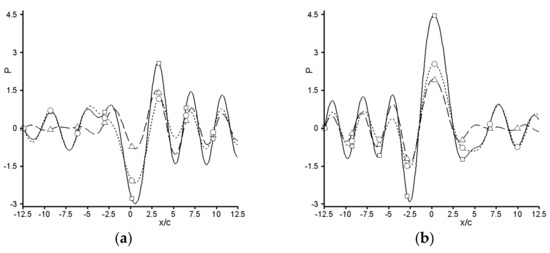
Figure 3.
Low frequency (St = 0.294) noise radiation from the trailing edge of an airfoil set at relatively high incidence (α = 20°). Instantaneous pressure fields, as recorded along the top (a) and bottom (b) walls. Incident field (), long dashes with delta symbols), all reflected fields (, small dashes with circle symbols), total field (, solid line with square symbols). For visualization purposes, the pressure fields are here normalized by Amax.
As can be seen, the interplay between the incident and reflected fields is more or less important, depending on the location. For some points (e.g., x/c ~ 0.5 on bottom wall), it induces constructive interferences, thereby leading to a resulting (total) pressure field that is almost twice as its original (incident) counterpart. The opposite occurs in other locations (e.g., x/c ~ −0.75 on top wall), where the interferences are destructive, i.e., the reflected field cancels the incident one, thus leading to an overall total pressure that is nil.
Obviously, the above observations are made at a specific moment of the source emission (t = 10T), which may not reflect what happens over time. To answer this point, an integrated measure is needed, which is introduced hereafter through the Root Mean Square (RMS) pressure.
2.3. Root Means Square (RMS) Pressure
2.3.1. RMS Pressure Field
The RMS (Root Mean Square) pressure represents the time-integrated value of the noise field, or its acoustical energy. It is classically defined by:
When developing the total field (, cf. Equation (1)), one gets
The first and second terms respectively correspond to the incident and reflected fields, whose interaction is given by the third term. By further developing the reflected field (, cf. Equation (6)), one gets
Recasting the latter expression into Equation (51) leads to
or, written in terms of the sole (real and virtual) sources’ pressure field, (cf. Equations (2), (7) and (15)),
By integrating the latter quantity over one source period, one then readily obtains the RMS field in any point of the domain (see Equation (50)). Notably, although such an integration can be performed numerically, one can also derive it via analytical means, as is done hereafter for the present case of a harmonic dipolar source.
2.3.2. Particular Case of a Harmonic Dipolar Source
Incident, Reflected and Total RMS Pressure Fields
First, one can note that all terms in Equation (54) can be expressed under a similar form (with and )
In the above equation, and relate to the source directivity and wavenumber, respectively. The former term is given by
On the other hand, the second term is expressed as
From there, one gets
and
All in all, this leads to,
i.e.,
or
In the above identity, the three first terms under the square root translate the contribution of the incident and the two reflected fields, respectively. The three last terms rather translate the interferences between these various fields, with either reinforcement or cancellation effects.
Here, it is worth noticing that the three terms associated with either the incident or the reflected fields do not depend on the source frequency, but solely on its location, via (, ). Oppositely, the three terms associated with these fields’ interferences are driven by both the source location and frequency (via the wavenumber, ). Finally, the amplitude term, , solely depends on the frequency (via the pulsation, ω).
Incident, Reflected and Total RMS Pressure Fields at the Wall
For an observer that would be located on the top wall, the resulting overall RMS pressure can be obtained by either applying to Equation (48) the time integration of Equation (50) or, more simply, by recasting Equation (64) using the particular identities and that are verified at the wall (see Section 2.2.4). This leads to
Similarly, for an observer that would be located on the bottom wall, the resulting overall RMS pressure is derived from Equation (49) (along with Equation (50)) or by recasting Equation (64) such that and (see Section 2.2.4).
The above Equations (64)–(66) constitute the primary methodological outcome of the present study. They allow predicting in a straightforward manner what would be the resulting acoustic field to occur within and along the walls of a 2D vein, should a harmonic dipolar noise of frequency (f) be radiated from the trailing edge of an airfoil set at an incidence (α). By extension, these equations offer discriminating the field’s various components (e.g., incident, reflected), so as to isolate the installation effects incurred by the vein and, thus, to assess their impact on the noise measurements. This point is illustrated hereafter.
2.3.3. Illustration via a Test Case
Still regarding the previous test case, Figure 4 depicts the RMS pressure fields recorded within the vein. As previously, each component is isolated on purpose, e.g., the incident field, the reflected fields along with their various interactions, and the resulting total field. Again, the latter differ significantly from the former (compare for instance Figure 4a–d), both quantitatively (higher amplitude levels) and qualitatively (more complex patterns).
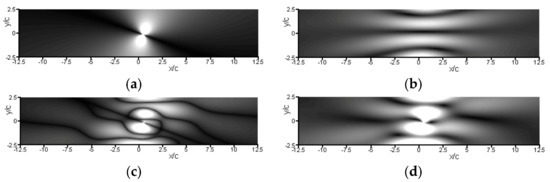
Figure 4.
Low frequency (St = 0.294) noise radiation from the trailing edge of an airfoil set at relatively high incidence (α = 20°). RMS pressure fields: (a) Incident field (1st term in Equation (64)); (b) top plus bottom wall reflected fields and their interaction (2nd, 3rd and last term in Equation (64); (c) incident and reflected fields’ interaction (4th and 5th terms in Equation (64)); (d) total field (, all terms in Equation (64)). For visualization purposes, all RMS pressure fields are normalized by Amax and depicted over an amplitude range [0; 2] using 60-iso contours.
To assess more precisely their differences, Figure 5 depicts the deltas (in dB) between the incident and total RMS pressure fields. As revealed by this map, the installation effects can be significant depending on the observer location, with deltas ranging from −15 dB (cf. the blue zones) to more than 30 dB (cf. the white areas). Notably, the impact is higher in those regions which originally corresponded to the shadow zone of the dipole, namely along its axis (i.e., the projected airfoil centerline). There, the rise of amplitude levels incurred by both the reflection and interference effects leads to deltas of up to 60 dB in some points, to begin with those located along the walls.
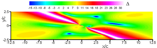
Figure 5.
Low frequency (St = 0.294) noise radiation from the trailing edge of an airfoil set at relatively high incidence (α = 20°). Deltas (in dB) between the incident and total RMS pressure fields.
This is more visible in Figure 6, which depicts both the incident and the total RMS pressures recorded along the top and bottom walls (cf. Figure 6a and Figure 6b, respectively), as well as their associated deltas (cf. Figure 6c). Here again, one can see how the incident pressure is modulated by its reflected counterparts and their subsequent interaction, thereby leading to an entirely different total RMS pressure. When considering for instance those points where the incident pressure is maximum (x/c ~ 0.8 and x/c ~ 0.0 of the top and bottom walls, respectively), the total field appears to be roughly 2.5 times more important, thereby leading to a delta of approx. +8 dB. Interestingly (even though logically) enough, it is rather in those locations where the incident pressure is close to zero that the delta skyrockets (see for instance what happens at points |x/c| ~ 7 on top and bottom walls, where deltas reach +60 dB and +58 dB, respectively).
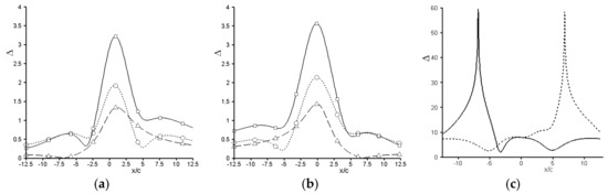
Figure 6.
Low frequency (St = 0.294) noise radiation from the trailing edge of an airfoil set at relatively high incidence (α = 20°). Left (a) and center (b) side, respectively: RMS pressure recorded along the top and bottom walls (depicted in linear scale, once normalized by Amax). Incident field (long dashes with delta symbols), all reflected fields (small dashes with circle symbols) and total field (solid line with square symbols). Right side (c): Deltas (in dB) between the incident and total RMS pressure fields, as recorded along both the top (solid lines) and bottom (dashes) walls.
The above results illustrate well how importantly the reverberation effects can alter the TE noise signature, thereby potentially biasing its in situ measurement using flushed mounted wall microphones.
At this stage, however, it is worth noticing that these results are specific to the present test case and should not be readily extended to other situations for which the TE source would differ from the present one, whether in terms of nature (harmonic dipole), frequency (St = 0.294) and/or location (i.e., airfoil chord and incidence, c = h/2.5, α = 20°). Exploring alternative situations is the matter of the next section.
3. Parametric Investigation
The present section focuses on the variability of the vein’s installation effects onto the acoustic signature to be measured by wall-mounted microphones, depending on the TE noise characteristics, i.e., its location (α) and/or frequency (St). To do so, a parametric investigation is conducted using the formalism introduced above, the previous test case being extended so as to cover a wider range of incidences (α up to 25°) and frequencies (St up to 3). The reason for exploring these particular ranges of flow incidence and noise frequency is that they are representative of typical small-scale experiments focusing on airfoil self-noise, such as those by Brooks et al. [1] (who explored a similar range, i.e., α ≤ 25° and f ≤ 10 kHz).
3.1. Varying the TE Noise Source Location and/or Frequency
The variability of the delta effects with respect to the sole TE noise source location (i.e., airfoil incidence) is assessed first. To do so, the previous case of a low frequency source (St = 0.294) is considered again, the angle of attack being now varied from α = 0° to α = 25° by increments of Δα = 5°. Figure 7 depicts the corresponding deltas between the incident and total RMS pressure fields, as recorded along both the top and bottom walls. Of note, given the symmetry of the problem, cases of negative incidences (α = 0° → −25°) would deliver identical outcomes, except that top and bottom walls results would be inverted. In other words, the delta effects to be recorded on the top (resp. bottom) wall for a negative α would match those acquired on the bottom (resp. top) wall for its positive |α| counterpart. As can be seen, the deltas exhibit similar albeit distinct patterns, depending on the incidence. One can first notice that only the case α = 0° sees the deltas of its top and bottom walls perfectly mirroring each other. This naturally results from the combined effect of a perfectly symmetric configuration (uninclined airfoil) and a perfectly antisymmetric noise emission (dipolar source). Contrarily, all other cases (α ≠ 0°) are characterized by delta effects that do not mirror each other, which comes from the broken symmetry of the configuration (inclined airfoil).
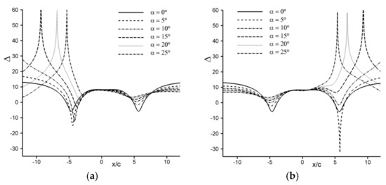
Figure 7.
Low frequency (St = 0.294) noise radiation from the trailing edge of an airfoil set at low to high incidences (α = 0°, 5°, 10°, 15°, 20°, 25°). Deltas (in dB) between the incident and total RMS pressure fields, as along the top (a) and bottom (b) walls.
At moderate to high incidences (α = 15° to 25°), one recovers the patterns previously observed for the α = 20° case (which is reproduced here in grey color, for reference). In particular, one retrieves the delta peak of up to +60 dB impacting the top (resp. bottom) wall upstream (resp. downstream) the airfoil, whereas moving away from it as the incidence decreases. Again, this peak reflects the walls backscattering effect onto that shadow zone which initially characterized the incident field along the airfoil chord line (cf. Figure 4 and Figure 5). Logically, as the airfoil incidence decreases, this peak travels away, up to disappearing beyond the |x|/c = 12.5 limit when α gets down to 10°.
At lower incidences (α = 10° to α = 0°), whilst the +60 dB delta peak is no longer visible, a negative delta peak is seen to appear at x/c ~ −4.75 and x/c ~ 5.75 on top and bottom walls, respectively. This peak is more importantly pronounced for an incidence of α = 5°, exhibiting an amplitude of approximately −10 dB and −30 dB on the top and bottom walls, respectively. Such a negative delta effect finds its origin in the reciprocal cause of the previous positive +60 dB peak; whereas the latter originated from the constructive interferences between the incident and reflected fields, here, it is rather their destructive counterparts that are at play, resulting in an overall pressure that is less than originally.
This effect is especially more visible in Figure 8 and Figure 9, which depict the corresponding incident and total pressure fields (cf. Figure 8), as well as their associated deltas (cf. Figure 9). There, one can clearly see how the confined acoustic field is driven by all constructive and destructive interferences (cf. Figure 8b), which then result in areas where the total RMS pressure is less than its incident counterpart (compare for instance Figure 8c,d). Subsequently, their delta turns negative over a few spatially distributed zones (cf. Figure 9), some of which extend up to the top and bottom walls, thereby explaining the peculiarities of Figure 7.
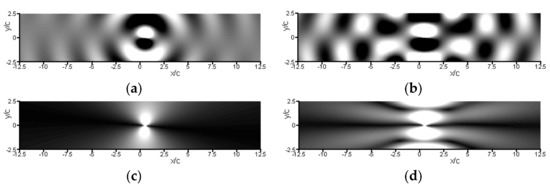
Figure 8.
Low frequency (St = 0.294) noise radiation from the trailing edge of an airfoil set at low incidence (α = 5°). Top: Instantaneous pressure field recorded within the vein after 10 source periods, depicted as incident (a) and total (b) components. Bottom: corresponding RMS pressure field, with incident (c) and total (d) components. For visualization purposes, all pressure fields are normalized by Amax and depicted using 60-iso contours distributed over an amplitude range of [−1; 1] (a,b) and [0; 2] (c,d).
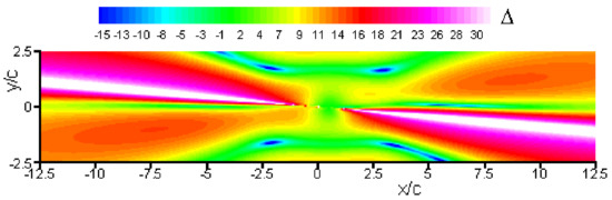
Figure 9.
Low frequency (St = 0.294) noise radiation from the trailing edge of an airfoil set at low incidence (α = 5°). Deltas (in dB) between the incident and total RMS pressure fields.
In addition to its sole location, the impact of the TE noise source frequency is also explored. To this end, the previous assessment of the airfoil incidence effect onto the low-frequency TE noise (St = 0.294, cf. Figure 8) is repeated for three different frequencies (St = 0.882, 1.47, 2.94). For each case, Figure 10 depicts the deltas between the incident and total RMS pressure fields, as recorded along either the top or the bottom walls. At first sight, the patterns appear to be rather conservative throughout all frequencies. In particular, in its upstream (resp. downstream) part, the top (resp. bottom) wall is systematically impacted by the +60 dB delta peaks, which emerge for the same higher incidences (α = 15°, 20°, 25°). This is coherent with the fact that this peak originates from the incident field’ shadow zone, whose location depends solely on the dipole inclination, whatever the frequency is. Oppositely, the negative delta peaks see their number as well as their respective amplitudes and locations varying importantly with the frequency. This is in line with the fact that these peaks rather relate to the interference effects, which were shown to depend on both the source location and frequency (cf. Section 2.3.2). In particular, more and more of these negative peaks emerge as the source frequency increases, due to the many more noise waves (of shorter wavelengths) and, thus, subsequent interference effects. Consequently, at higher frequencies, the resulting deltas (i.e., installation effects) undergo much quicker variations along both the top and bottom walls. This may complexify the identification of those particular wall locations where to better position a flush-mounted microphone, should in situ noise measurements be conducted.
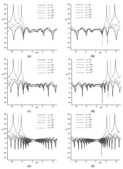
Figure 10.
Moderate to high frequency (St = 0.882, 1.47, 2.94) noise radiation from the trailing edge of an airfoil set at low to high incidences (α = 0°, 5°, 10°, 15°, 20°, 25°). From top to bottom: St = 0.882 (a,b), St = 1.47 (c,d), St = 2.94 (e,f). Deltas (in dB) between the incident and total RMS pressure fields, as recorded along the top (left: a,c,e) and bottom (right: b,d,f) walls.
To explore that point, the variability of the wall-recorded deltas towards the source frequency is investigated in a more systematic manner. For all given incidences (α = 0°, 5°, 10°, 15°, 20°, 25°), Figure 11 depicts the top and bottom walls’ respective RMS delta as a function of the source frequency (St = 0.0147 to 2.94, with ΔSt = 0.03675). First, one can see again that whatever the frequency is, the +60 dB delta peaks emerge when the incidence is high enough (α > 10°), whereas moving towards the airfoil as it further increases. One can then observe again that whatever this incidence is, the deltas alternate from positive to negative values as the observer moves along each wall, with such alternance occurring more quickly as the frequency increases. Finally, one can see that, whatever the frequency and incidence are, these deltas are less important on the top (resp. bottom) wall region such that (resp. ).
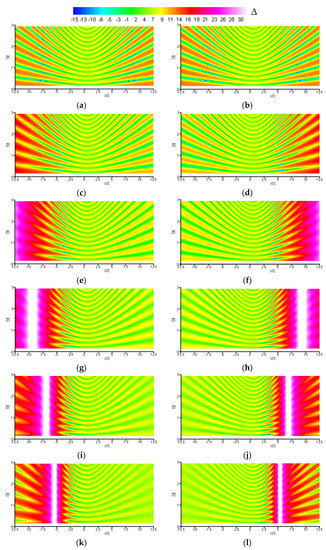
Figure 11.
Low to high frequency (St = [0.0147; 2.94]) noise radiation from the trailing edge of an airfoil set at low to high incidences (from top to bottom): α = 0° (a,b), α = 5° (c,d), α = 10° (e,f), α = 15° (g,h), α = 20° (i,j), α = 25° (k,l). Deltas (in dB) between the incident and total RMS pressure fields, as recorded along the top (left: a,c,e,g,i,k) and bottom (right: b,d,f,h,j,l) walls.
From this, one can conclude that these two areas are the optimal zones where to position a flush-mounted microphone, should in situ noise measurements be conducted. At this stage, however, it is worth noting that it is custom to locate microphones downstream the airfoil (x/c > 0), if only for avoiding the multiple backscattering to possibly occur between the mock-up and each wall. In conclusion, whatever the frequency and (positive) incidence is, the microphone should ideally be located on the top wall, at a position such that (please note that a negative incidence would lead to opposite trends, i.e., the microphone should rather be positioned on the bottom wall, still such that .) Further assessing this observation is the matter of the next subsection.
3.2. Characterizing the Installation Effects on Flush-Mounted Microphones Located Right Downstream the Trailing Edge
To further assess what would be the ideal location(s) where to position a flush-mounted microphone, the present section focuses on these top and wall regions such that .
3.2.1. Characterization of the Installation Effects
Figure 12 depicts the corresponding RMS deltas, as recorded for three specific frequencies (St = 0.294, 1.47, 2.94) and all five incidences (α = 0° to 25°).
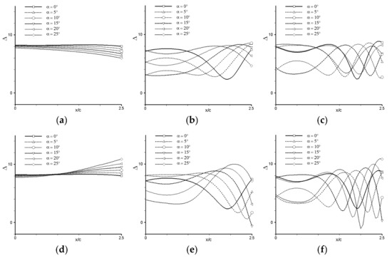
Figure 12.
Low to high frequency (St = 0.294, 1.47, 2.94) noise radiation from the trailing edge of an airfoil set at low to high incidences (α = 0°, 5°, 10°, 15°, 20°, 25°). From left to right: St = 0.294 (a,d), St = 1.47 (b,e), St = 2.94 (c,f). Deltas (in dB) between the incident and total RMS pressure fields, as recorded along the top (up: a–c) and bottom (down: d–f) walls.
Overall, it appears that there is no specific location for which the RMS deltas are minimum at all angles and frequencies considered. In particular, it is again confirmed that the top wall is somehow less impacted than the bottom wall (the opposite would hold for negative incidences). More precisely, for points that are located less than a chord away downstream the source (x/c < 1.5), the top and bottom walls are affected in a similar manner. In particular, at low frequency (St = 0.294), the delta is roughly constant whatever the airfoil incidence is, namely Δ ~ +8 dB for both walls. At moderate (St = 1.47) and high (St = 2.94) frequencies, this delta varies with the incidence whereas staying within similar bounds (Δ ~ +3.5 dB to +8 dB for both walls). Oppositely, for points that are located further downstream (x/c > 1.5), the top and bottom walls are impacted differently; whereas their deltas go on varying with the incidence (α), such variation is less for the top wall (Δ ~ 2 dB to 9 dB) compared to its bottom counterpart (Δ ~ −1 dB to 11 dB). Based on the above observations, one can infer that a microphone should preferably be located on the x/c < 1.5 portion of either the top or the bottom wall, thereby being impacted less, overall. Oppositely, the worse location would correspond to a microphone located on the x/c > 1.5 portion of the bottom wall, thereby suffering from deltas with a higher variability, depending on the (positive) incidence and frequency.
To further assess and illustrate this point, two pairs of microphones are considered; the first pair of microphones (M1±) is positioned such that = 0.5, i.e., they are located right at the zenith of the airfoil TE location, on either the top or bottom wall (M1+ and M1−, respectively). The second pair of microphones (M2±) is located approximately 1.5 chord downstream the TE, i.e., = 2, being also positioned on either the top or bottom wall (M2+ and M2−, respectively). For each microphone, Figure 13 depicts the delta between the incident and the total RMS pressure fields, plotted here as a function of both the airfoil incidence (α) and the source frequency (St). From a qualitative viewpoint, both pairs of microphones exhibit an identical pattern, namely a regular oscillation of their associated RMS delta as the source frequency (St) increases. Notably, for the two microphones located on the top wall (M1+ and M2+), these oscillations get slightly slower when the incidence increases, whereas the opposite is true for their bottom wall counterparts (M1− and M2−). From a quantitative perspective, the downstream microphones (M2±) appear to exhibit higher deltas than their upstream counterpart (M1±), although this depends on the airfoil incidence (i.e., source location).
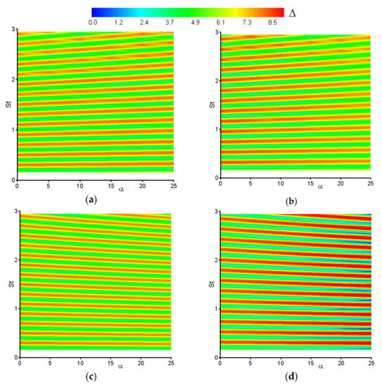
Figure 13.
Low to high frequency (St = [0.294; 2.94]) noise radiation from the trailing edge of an airfoil set at low to high incidences (α = [0°; 25°]). Deltas (in dB) between the incident and total RMS pressure fields, as recorded for two pairs of microphones: M1± (= 0.5) and M2± ( = 2) located on top and bottom walls: M1+ (a), M1− (c), M2+ (b), M2− (d).
To illustrate this point better, Figure 14 depicts again the RMS delta recorded at each four microphones, this delta being now plotted as a function of the sole source frequency (St), for either a nil (α = 0°) or a high (α = 25°) incidence. In other words, Figure 14 displays two α-cuts excerpted from Figure 13, each being associated with one of the two extrema in incidence. For the top wall microphone M1+, when the airfoil incidence is nil (α = 0°), the RMS delta oscillates between Δmin = 3.0 dB and Δmax = 8.0 dB, cycling over a range of frequencies that is about ΔSt ~ 0.2. Notably, this delta reaches a minimum (resp. maximum) for source frequencies such that Stmin ~ 0.2 mod(ΔSt) (resp. Stmax ~ 0.3 mod(ΔSt)). Differently, when the airfoil incidence is high (α = 25°), even though the delta remains of same amplitude, its oscillation frequency shifts towards ΔSt ~ 0.22 whereas its minimum and maximum peaks move to Stmin ~ 0.22 mod(ΔSt) and Stmax ~ 0.33 mod(ΔSt), respectively. Considering now the bottom wall microphone M1−; at zero incidence (α = 0°), its RMS delta matches that of its top wall counterpart (Δmin ~ 3.2 dB, Δmax ~ 8.2 dB, ΔSt ~ 0.2), which can be explained by obvious symmetry reasons (uninclined airfoil). On the other hand, when set at a high incidence (α = 25°), its RMS delta is seen to oscillate less importantly (Δmin ~ 3.2 dB, Δmax = 8.0 dB) and over a shorter cycle of frequencies (ΔSt ~ 0.185). Looking then at the downstream pair of microphones M2±; when the airfoil is again free of any incidence (α = 0°), they both experience an identical RMS delta, which oscillates slightly more importantly in amplitude (Δmin ~ 2.5 dB, Δmax = 8.5 dB) and rapidly in frequencies (ΔSt ~ 0.211), compared to that of their M1± counterpart. Finally, when the airfoil is put at high incidence (α = 25°), the top wall microphone M2+ exhibits a RMS delta that oscillates much less (Δmin ~ 3.6 dB, Δmax = 8.0 dB) albeit more rapidly (ΔSt ~ 0.23), compared to its bottom wall counterpart M2− (Δmin ~ −1 dB, Δmax = 9.75 dB, ΔSt ~ 0.198).
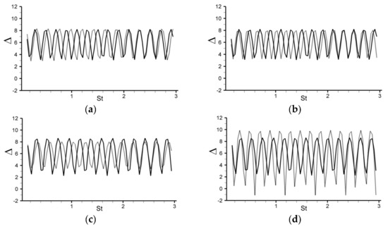
Figure 14.
Low to high frequency (St = [0.294; 2.94]) noise radiation from the trailing edge of an airfoil set at low (α = 0°, solid line) or high (α = 25°, dashed line) incidences. Deltas (in dB) between the incident and total RMS pressure fields, as recorded for two pairs of microphones: M1± (= 0.5) and M2± ( = 2) on top and bottom walls: M1+ (a), M1− (c), M2+ (b), M2− (d).
The above results illustrate the high variability of the acoustic installation effects, which depend not only on the noise source characteristics (location, frequency), but also on the microphone position. The reason behind this is explored in the next subsection.
3.2.2. Interpretation of the Installation Effects
The above oscillations of the RMS delta can be explained by the alternance of constructive and destructive interferences between the incident and reflected fields that reach the microphones. Indeed, depending on the TE noise source frequency (i.e., wavelength) and location (i.e., propagation distance), each microphone will see these incident and reflected waves reaching it with a specific phase delay. Whenever the waves are perfectly in phase, their amplitude will sum up and the RMS delta will be higher. Contrarily, if some waves are in phase opposition, they will partly cancel each other, thereby reducing the RMS delta.
For the top (resp. bottom) wall microphones, this effect can be inferred using Equation (65) (resp. Equation (66)). In this equation, the two first terms are balanced by a third one, which involves a quantity (with and for the top and bottom walls, respectively). This quantity varies between 1 and −1, depending on the values taken by the 2π-modulo remainder of . The latter term is driven by the difference in the propagation paths between the incident and reflected waves, which ultimately translates into possible phase delays. Indeed, considering that the wave number is with λ the wavelength, one has . The phase delay and subsequent interference effect thus depends on how the difference in propagation paths scales with the wavelength. For instance, whenever the former is an exact multiple of the latter (, then , i.e., the RMS delta is minimized (given the negative sign of the cosines product, cf. Equations (65) and (66)). Oppositely, when the difference in propagation paths is an odd multiple of half the wavelength ( then , and the RMS delta is maximized (cf. Equations (65) and (66)). As an illustration, let us consider the particular (and simplest) case of M1± microphones ( when the airfoil is put at no incidence (α = 0), i.e., the source is located at , . Considering that, in the present case b = c/2 as well as c = h/2.5 (cf. Section 2.2.6), the top wall microphone M1+ is such that (cf. Equations (29), (31) and (65))
and
On the other hand, its bottom wall counterpart M1− is such that (cf. Equations (34), (35) and (66))
and
Therefore, for both microphones, the difference in propagation paths becomes Consequently, their RMS delta will be minimum for source frequencies such that , i.e., , with m = 1, 2, …, etc. The lowest one corresponds to m = 1, i.e., λ = 2h. Considering the present Strouhal definition ( and the fact that , this gives St = 1/5 = 0.2, which matches with the above observations, Stmin ~ 0.2 mod(ΔSt). Oppositely, the RMS delta will be maximum for source frequencies such that + 1)/2, i.e., , with m = 1, 2, …, etc. The lowest one corresponds to m = 1, i.e., λ = 4h, i.e., St = 1/10 = 0.1, which matches with the above observations (Stmax ~ 0.3 = 0.1 mod(ΔSt)).
Obviously, the above relationships become less trivial when the airfoil is put at incidence (α ≠ 0), with the source now located at . For instance, considering again the top wall microphone, one gets (with, again, b = c/2)
and
Considering again that c = h/2.5, this leads to
As an illustration, in the high incidence case (α = 25°), the difference in propagation paths associated with the top microphone now becomes . The RMS delta will thus oscillate over a cycle in frequencies such that , i.e., , i.e., St = c/λ = 1/(2.5 × 1.83) = 0.218, which coincides with the previous observations (ΔSt ~ 0.22).
Similar analyses can be made for the other pair of microphones M2± and/or different incidences, which are not detailled here for the sake of conciseness.
All the above observations further illustrate how the acoustic installation effects induced by the vein confinement may affect the TE noise signature, as well as its subsequent measurement using flush-mounted microphones. Additionally, they also exemplify how this bias can be assessed in a rather straightforward manner, so as to be prevented a priori or corrected a posteriori.
4. Conclusions
With respect to the mitigation of the environmental noise of aerodynamic origin, the present study aims at enabling the experimental characterization of airfoil noise using closed-vein, aerodynamic wind tunnels. The latter facilities are indeed known to restitute better the aerodynamic flow features (and, thus, noise sources), but at the price of incurring important acoustic installation effects, namely, reverberation by the duct’s walls. This question is here explored with respect to the specific albeit important problem of the aerodynamic noise generated by the trailing edge (TE) of airfoils, when the latter are sunk into low-to-moderate Reynolds number flows. To this end, an analytical model is derived, which allows predicting the wall-induced reverberation effects that an as-like airfoil TE noise source (2D harmonic dipole) shall be subjected to, when radiating within a closed-vein, hard-wall, wind tunnel. This is exemplified through a representative test case, which is then explored through a parametric study, thereby allowing to illustrate better how these acoustic installation effects may impact the noise measurements that would be performed using flush-mounted microphones located on the vein’s walls.
From a phenomenological perspective, the study highlights how important the reverberation effects by the vein can be, depending on the TE noise source location (i.e., airfoil incidence) and, to a lesser extent, its frequency. In particular, it is shown how these effects may impact very diversely any given flush-mounted microphone, depending on its position. As demonstrated here, this results from the (constructive or destructive) noise interferences inherited from the way the acoustic wavelength (i.e., TE noise frequency) combines with the propagation distance (i.e., TE and microphone respective locations).
From a methodological viewpoint, the study illustrates how the acoustic installation effects incurred by the vein can be straightforwardly assessed, using the proposed analytical formalism. The latter may thus constitute a useful diagnosis tool for mitigating the experimental biases that would weigh on airfoil TE noise tests to be performed within a closed-vein facility, whether by preventing them a priori (e.g., exploring where to better locate the flush-mounted microphones) or by remedying them a posteriori (e.g., de-biasing the noise measurements accordingly).
Of course, the simplicity of the proposed analytical formalism comes at the price of some underlying assumptions. First, as of now, the approach solely incorporates those acoustic installation effects which are incurred by the vein’s walls (reverberation), excluding those that may be induced by the flow (e.g., convection, refraction). Second, only primary specular reflections are considered here, all secondary ones being neglected. Although these approximations are deemed to be very acceptable in regard to the particular problem that is considered here (airfoil TE noise), relaxing these two constraints constitute the immediate perspective of this work.
Funding
This research received no external funding.
Conflicts of Interest
The author declares no conflict of interest.
Appendix A. Derivation of the RMS Expression
Starting from the trigonometric relation , it is easy to show that
and
Additionally, if one sets a = b, one also gets
First, let us evaluate
with , by definition. One knows that
Therefore
since periodicity imposes that
Therefore
From the trivial relationship
One immediately gets
Through integration by parts, it’s easy to show that
Therefore
All in all, by Equations (A3), (A8), (A10) and (A12), one gets
On the other hand, by Equations (A2), (A8), (A10) and (A12), one gets
References
- Brooks, F.; Stuart, D.; Marcolini, A. Airfoil Self-Noise and Prediction; NASA Technical Report 1218; National Aeronautics and Space Administration, Office of Management, Scientific and Technical Information Division: Washington, DC, USA, 1989. [Google Scholar]
- Arcondoulis, E.; Doolan, C.; Zander, A.; Brooks, L. A review of Trailing Edge Noise Generated by Airfoils at Low to Moderate Reynolds Number. Acoust. Aust. 2010, 38, 135–139. [Google Scholar]
- Golubev, V. Recent Advances in Acoustics of Transitional Airfoils with Feedback-Loop Interactions: A Review. Appl. Sci. 2021, 11, 1057. [Google Scholar] [CrossRef]
- Clark, L.T. The Radiation of Sound From an Airfoil Immersed in a Laminar Flow. J. Eng. Power 1971, 93, 366–376. [Google Scholar] [CrossRef]
- Paterson, R.W.; Vogt, P.G.; Fink, M.R.; Munch, C.L. Vortex Noise of Isolated Airfoils. J. Aircr. 1973, 10, 296–302. [Google Scholar] [CrossRef]
- Nash, E.C.; Lowson, M.V.; McAlpine, A. Boundary-layer instability noise on aerofoils. J. Fluid Mech. 1999, 382, 27–61. [Google Scholar] [CrossRef]
- McAlpine, A.; Nash, E.; Lowson, M. On the Generation of Discrete Frequency Tones by the Flow around an Aerofoil. J. Sound Vib. 1999, 222, 753–779. [Google Scholar] [CrossRef]
- Moreau, S.; Henner, M.; Iaccarino, G.; Wang, M.; Roger, M. Analysis of Flow Conditions in Free-jet Experiments for Studying Airfoil Self-Noise. AIAA J. 2003, 41, 1895–1905. [Google Scholar] [CrossRef]
- Nakano, T.; Fujisawa, N.; Oguma, Y.; Takagi, Y.; Lee, S. Experimental study on flow and noise characteristics of NACA0018 airfoil. J. Wind. Eng. Ind. Aerodyn. 2007, 95, 511–531. [Google Scholar] [CrossRef]
- Atobe, T.; Tuinstra, M.; Takagi, S. Airfoil Tonal Noise Generation in Resonant Environments. Trans. Jpn. Soc. Aeronaut. Space Sci. 2009, 52, 74–80. [Google Scholar] [CrossRef][Green Version]
- Hansen, K.; Kelso, R.; Doolan, C. Reduction of Flow Induced Tonal Noise Through Leading Edge Tubercle Modifications. In Proceedings of the 16th AIAA/CEAS Aeroacoustics Conference, Stockholm, Sweden, 7–9 June 2010. [Google Scholar] [CrossRef]
- Plogmann, B.; Herrig, A.; Würz, W. Experimental investigations of a trailing edge noise feedback mechanism on a NACA 0012 airfoil. Exp. Fluids 2013, 54, 1–14. [Google Scholar] [CrossRef]
- Devenport, W.J.; Burdisso, R.A.; Borgoltz, A.; Ravetta, P.A.; Barone, M.F.; Brown, K.; Morton, M.A. The Kevlar-walled anechoic wind tunnel. J. Sound Vib. 2013, 332, 3971–3991. [Google Scholar] [CrossRef]
- Moreau, D.J.; Doolan, C.J. Tonal noise production from a wall-mounted finite airfoil. J. Sound Vib. 2016, 363, 199–224. [Google Scholar] [CrossRef]
- Tam, C.K.W. Discrete tones of isolated airfoils. J. Acoust. Soc. Am. 1974, 55, 1173–1177. [Google Scholar] [CrossRef]
- Longhouse, R. Vortex shedding noise of low tip speed, axial flow fans. J. Sound Vib. 1977, 53, 25–46. [Google Scholar] [CrossRef]
- Arbey, H.; Bataille, J. Noise generated by airfoil profiles placed in a uniform laminar flow. J. Fluid Mech. 1983, 134, 33–47. [Google Scholar] [CrossRef]
- Kingan, M.J.; Pearse, J.R. Laminar boundary layer instability noise produced by an aerofoil. J. Sound Vib. 2009, 322, 808–828. [Google Scholar] [CrossRef]
- Yakhina, G.; Roger, M.; Moreau, S.; Nguyen, L.; Golubev, V. Experimental and Analytical Investigation of the Tonal Trailing-Edge Noise Radiated by Low Reynolds Number Aerofoils. Acoustics 2020, 2, 293–329. [Google Scholar] [CrossRef]
- Salas, P.; Moreau, S. Aeroacoustic Simulations of a Simplified High-Lift Device Accounting for Some Installation Effects. AIAA J. 2017, 55, 1–16. [Google Scholar] [CrossRef]
- Desquesnes, G.; Terracol, M.; Sagaut, P. Numerical investigation of the tone noise mechanism over laminar airfoils. J. Fluid Mech. 2007, 591, 155–182. [Google Scholar] [CrossRef]
- Jones, L.E.; Sandberg, R. Numerical analysis of tonal airfoil self-noise and acoustic feedback-loops. J. Sound Vib. 2011, 330, 6137–6152. [Google Scholar] [CrossRef]
- Zhang, Y.; Wu, X.; Li, W. Direct numerical simulations of tonal noise generation for a two-dimensional airfoil at low and moderate Reynolds numbers. In Proceedings of the 46th AIAA Fluid Dynamics Conference, Washington, DC, USA, 13–17 June 2016. [Google Scholar] [CrossRef]
- Ricciardi, T.R.; Arias-Ramirez, W.; Wolf, W.R. On secondary tones arising in trailing-edge noise at moderate Reynolds numbers. Eur. J. Mech. B/Fluids 2019, 79, 54–66. [Google Scholar] [CrossRef]
- Nguyen, L.; Golubev, V.; Mankbadi, R.; Yakhina, G.; Roger, M. Numerical Investigation of Tonal Trailing-Edge Noise Radiated by Low Reynolds Number Airfoils. Appl. Sci. 2021, 11, 2257. [Google Scholar] [CrossRef]
- Michel, U. On the systematic error in measurements of jet noise flight effects using open jet wind tunnels. In Proceedings of the 21st AIAA/CEAS Aeroacoustics Conference, Dallas, TX, USA, 22–26 June 2015. [Google Scholar] [CrossRef]
- Moreau, S.; Schram, C.; Roger, M. Diffraction Effects on the Trailing Edge Noise Measured in an Open-jet Anechoic Wind Tunnel. In Proceedings of the 13th AIAA/CEAS Aeroacoustics Conference (28th AIAA Aeroacoustics Conference), Rome, Italy, 21–23 May 2007. AIAA paper 2007-3706. [Google Scholar]
- Redonnet, S. Investigation of the acoustic installation effects of an open-jet anechoic wind tunnel using computational aeroacoustics. Appl. Acoust. 2020, 169, 107469. [Google Scholar] [CrossRef]
- Amiet, R. Correction of open jet wind tunnel measurements for shear layer refraction. In Proceedings of the 2nd Aeroacoustics Conference, Hampton, VA, USA, 24–26 March 1975. [Google Scholar] [CrossRef]
- Amiet, R. Refraction of sound by a shear layer. J. Sound Vib. 1978, 58, 467–482. [Google Scholar] [CrossRef]
- Morfey, C.; Joseph, P. Shear layer refraction corrections for off-axis sources in a jet flow. J. Sound Vib. 2001, 239, 819–848. [Google Scholar] [CrossRef]
- Bahr, C.J.; Brooks, T.F.; Humphreys, W.M.; Spalt, T.B.; Stead, D.J. Acoustic Data Processing and Transient Signal Analysis for the Hybrid Wing Body 14- by 22-Foot Subsonic Wind Tunnel Test. In Proceedings of the 20th AIAA/CEAS Aeroacoustics Conference, Atlanta, GA, USA, 16–20 June 2014. [Google Scholar] [CrossRef]
- Porteous, R.; Geyer, T.; Moreau, D.; Doolan, C. A correction method for acoustic source localization in convex shear layer geometries. Appl. Acoust. 2018, 130, 128–132. [Google Scholar] [CrossRef]
- Pereira, L.T.L.; Martini, F.; de Almeida, C.O.; Bent, P. Feasibility of measuring noise sources on a detailed nose landing gear at low-cost development. Appl. Acoust. 2021, 182, 108263. [Google Scholar] [CrossRef]
- Marx, D.; Aurégan, Y.; Bailliet, H.; Valière, J.-C. PIV and LDV evidence of hydrodynamic instability over a liner in a duct with flow. J. Sound Vib. 2010, 329, 3798–3812. [Google Scholar] [CrossRef]
- Bahr, C.J.; Hutcheson, F.V.; Stead, D.J. Unsteady Propagation and Mean Corrections in Open-Jet and Kevlar® Wind Tunnels. AIAA J. 2021, 1–12. [Google Scholar] [CrossRef]
- Castellini, P.; Sassaroli, A. Acoustic source localization in a reverberant environment by average beamforming. Mech. Syst. Signal Process. 2010, 24, 796–808. [Google Scholar] [CrossRef]
- Wang, L.; Liu, Y.; Zhao, L.; Wang, Q.; Zeng, X.; Chen, K. Acoustic source localization in strong reverberant environment by parametric Bayesian dictionary learning. Signal Process. 2018, 143, 232–240. [Google Scholar] [CrossRef]
- Zamponi, R.; Chiariotti, P.; Battista, G.; Schram, C.; Castellini, P. 3D Generalized Inverse Beamforming in wind tunnel aeroacoustic testing: Application to a Counter Rotating Open Rotor aircraft model. Appl. Acoust. 2020, 163, 107229. [Google Scholar] [CrossRef]
- Allen, J.H.; Vincenti, W.G. Wall Interference in a Two-Dimensional Wind Tunnel, with Consideration of the Effect of Compressibility; NACA report n 782; 1947. Available online: https://digital.library.unt.edu/ark:/67531/metadc279436/ (accessed on 5 August 2021).
- Xie, Y.; Liu, G.; Chen, D. Wall Interference Assessment of Two-Dimensional Wind Tunnel Test Using Panel Method. In Proceedings of the 2020 IEEE 3rd International Conference on Electronics Technology (ICET), Chengdu, China, 8–11 May 2020; pp. 386–391. [Google Scholar] [CrossRef]
- Schlinker, R.; Fink, M.; Amiet, R. Vortex noise from non-rotating cylinders and airfoils. In Proceedings of the 14th Aerospace Sciences Meeting, Washington, DC, USA, 26–28 January 1976. AIAA paper 76-81. [Google Scholar]
- Munin, A.G.; Prozorov, A.G.; Toporov, A.V. Experimental study of noise generated in a low-velocity flow. Sov. Phys. (Acoust.) 1992, 38. Available online: https://www.researchgate.net/publication/295448886_Noise_experimental_research_of_airfoil_flow_with_low_velocities (accessed on 5 August 2021).


Publisher’s Note: MDPI stays neutral with regard to jurisdictional claims in published maps and institutional affiliations. |
© 2021 by the author. Licensee MDPI, Basel, Switzerland. This article is an open access article distributed under the terms and conditions of the Creative Commons Attribution (CC BY) license (https://creativecommons.org/licenses/by/4.0/).