In this section, results of classification; temporal and spatial analysis; damage estimation at the county-, city-, and grid-level via three algorithms; and damage map validation are presented.
5.1. Classification
In this study, binary classification and multi-class classification have been done. Binary classification is used to classify messages into two classes of damage and non-damage so that their results can finally be used to estimate the earthquake damage. Multi-class classification is used to categorize messages to increase post-crisis situational awareness and to monitor the process of changing conditions over time and to determine the concentration of various topics in different locations.
For classification, the pre-processed data were divided into training and test data. Then, based on the training data of each trained classification model and then using the test data, the accuracy of the prediction models were evaluated.
For binary classification, the final dataset comprised 26,942 tweets that were manually labeled to produce the training dataset of 5038 (including 4031 non-damage and 1007 damage) tweets. This dataset was divided into two sections. 70% of them were used for training and 30% of them are used for testing. Precision, accuracy, recall, Kappa, and F-measure were used for evaluating the performance of binary classification algorithms.
Table 1 demonstrates the performance of Naive Bayes, SVM, and deep learning binary classification.
In
Table 1, precision and recall were obtained from the average of two damage and non-damage classes by equal weight. The results of
Table 1 show that the SVM algorithm performed better in all the indices and Naive Bayes algorithm performed poorly in all the indices. The deep learning algorithm also performed moderately in all of the indicators. However, its results were closer to SVM than to Naive Bayes.
For multi-class classification, Neguyan et al. [
16] datasets, including 14,006 earthquake-labeled tweets (Napa and Nepal earthquake labeled datasets (
https://crisisnlp.qcri.org/), accessed on 16 October 2019) were used to create the training dataset. This dataset was split into two categories—60% of them were applied for training and 40% of them were applied for testing. The results show SVM classifier accurately identified damage-related messages. Precision, accuracy, recall, Kappa, and F-measure were used for evaluating the performance of multi-class classification algorithms.
Table 2 demonstrates the performance of Naive Bayes, SVM, and deep learning multi-class classification.
In
Table 2, precision and recall were obtained from the average of all five classes by equal weight. The results of
Table 1 show that the SVM algorithm performed better in all the indices and maïve Bayes algorithm performed relatively poorly in all the indices. The deep learning algorithm also performed moderately in all of the indicators.
5.2. Temporal and Spatial Analysis
In this section temporal and spatial analysis are presented.
Individuals’ concerns about a disaster will vary as the disaster evolves. For example, at the beginning of an earthquake, most of the messages may be related to damage and infrastructure, followed by discussions about donations and endowments. The topics shared on social networks are almost an example of the public’s thoughts. In this study, temporal patterns of binary classification topics (damage and non-damage) and multi-class classification topics (injured, dead, and missing people; infrastructure; donation; response effort; and other relevant information) via three classification algorithms were investigated.
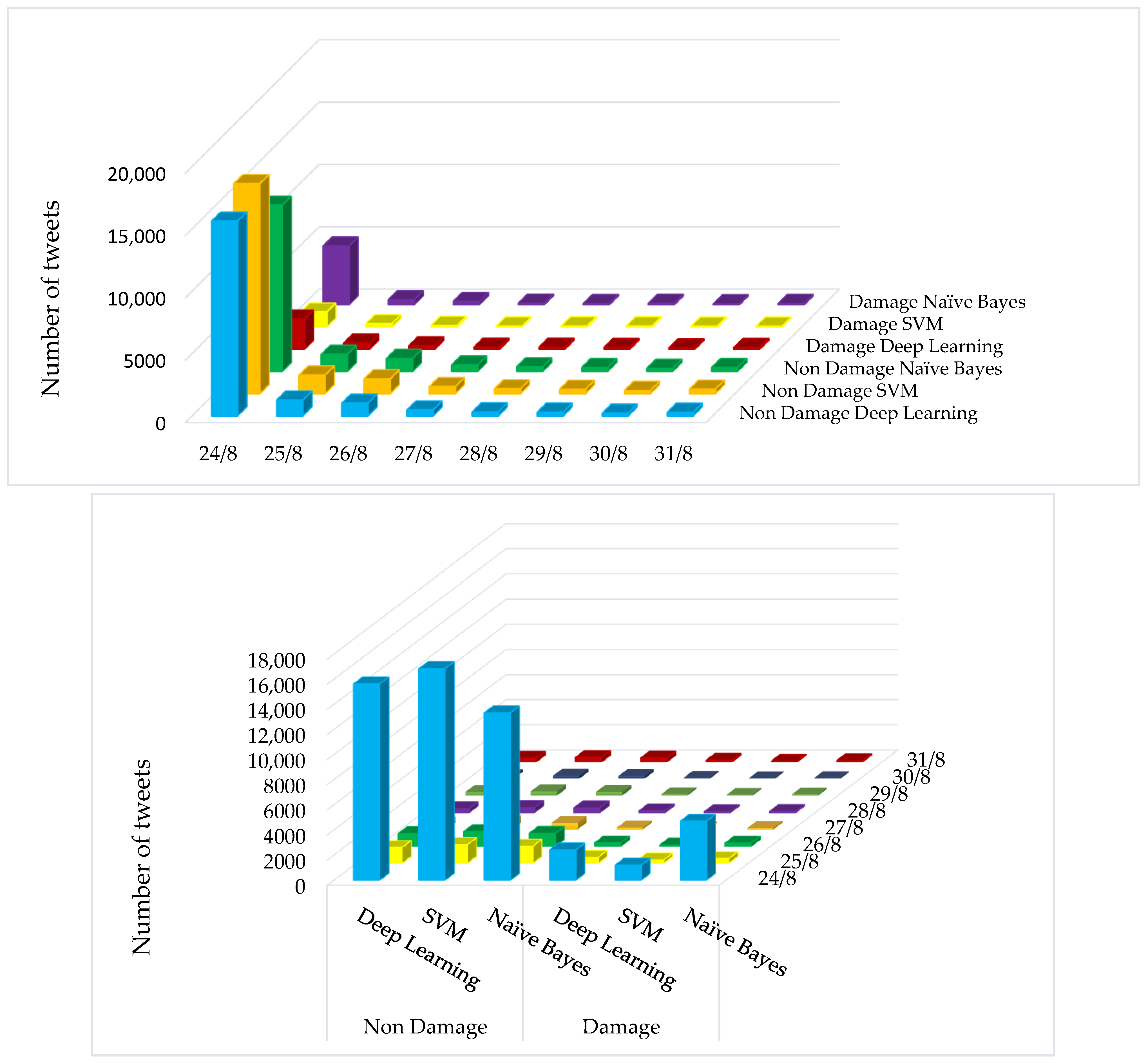
Figure 4 shows the number of tweets classified using three classification algorithms, Naive Bayes, SVM, and deep learning, on two classes of damage and non-damage on each day one week after the earthquake (August 24). Naive Bayes classification algorithm (
Figure 4) showed that among the tweets collected on the day of the earthquake, 26.05% of the tweets (4698 tweets) reported earthquake damage and the rest (13,336 tweets) did not report damage. In addition, most of the damage-related messages related to the earthquake day and decreased in the following days. In addition, the results of the SVM classification algorithm (
Figure 4) showed that among the tweets collected on the day of the earthquake, 6.61% of tweets (1193 tweets) reported earthquake damage and the rest of the tweets (16,841 tweets) did not report damage. After the day of the earthquake, 5185 tweets were collected, out of the tweets collected after the day of the earthquake, 12.44% of the tweets (645 tweets) showed damage caused by the earthquake and the rest (4540 tweets) reported no damage. The results of the deep learning algorithm (
Figure 4) also showed that 13.36% of tweets (2410 tweets) reported damage from earthquakes on the day of the earthquake and the rest of tweets (15,624 tweets) did not show damage. Among the tweets collected after the day of the earthquake, 25.86% of tweets (equivalent to 1341 tweets) reported damage caused by the earthquake and the rest of tweets (3844 tweets) did not show damage.
In general, in all three classification algorithms, most of the damage-related messages corresponded to the earthquake day and decreased in the following days. In addition, Naive Bayes extracted the most damage-related messages and SVM has extracted the least damage-related messages.
Figure 5 shows the distribution of tweets classified in five classes on each day a week before and after the earthquake (24 August) for the Naive Bayes, SVM, and deep learning classification algorithms. According to the results of Naive Bayes (
Figure 5), it can be seen that the tweets collected on the day of the earthquake had the lowest number of tweets for the “Injured_Dead_and_Missing_people”, “Donation”, and “Infrastructure” classes, respectively with 1.54 percent (279 tweets), 4.82 percent (869 tweets), and 5.27 percent (951 tweets). The highest number of tweets also belonged to the “Other_relevant_information” and “Response_efforts” classes, with 80.71% (14,556 tweets) and 7.64% (1379 tweets), respectively. In addition, among the tweets collected in the days following the earthquake, 0.62% (32 tweets), 0.73% (39 tweets), and 4.32% (224 tweets) belonged to the “Donation”, “Injured_Dead_and_Missing_people”, and “Infrastructure” classes, and 5.57% (289 tweets) and 88.74% (4601 tweets) tweets belonged to the “Injured_Dead_and_Missing_people” and “Other_relevant_information” classes, respectively. According to SVM algorithm results (
Figure 5), no tweets collected on the day of the earthquake were classified in the “Injured_Dead_and_Missing_people”, “Donation”, and “Infrastructure” classes. The number of tweets in the “Other_relevant_information” and “Response_efforts” classes was 99.97% (18,030 tweets) and 7.64% (1379 tweets), respectively, among the tweets collected on the day of the earthquake. The results of the deep learning model (
Figure 5) also showed that the number of tweets collected on the day of the earthquake had the lowest number of tweets for the “Donation”, “Infrastructure”, and “Response_efforts” classes, respectively, with 0.38% (104 tweets), 2.96% (797 tweets), and 6.62% (1779 tweets). The highest number of tweets also belonged to the “Other_relevant_information” and “Injured_Dead_and_Missing_people” classes, with 80.79% (21,711 tweets) and 9.23% (2482 tweets), respectively. In addition, the tweets collected in the days after the earthquake, amounting to of 0.6% (31 tweets), 4.38% (227 tweets), and 5.01% (260 tweets), related to classes “Donation”, “Infrastructure”, and “Response_efforts”, respectively. In addition, 5.09% (264 tweets) and 84.92% (4403 tweets) belonged to the classes “Injured_Dead_and_Missing_people” and “Other_relevant_information”, respectively.
Overall, most of the messages classified in the three algorithms were in the class “Other_relevant_information”. Additionally, most of the messages related to infrastructure damages and injured, dead, and missing people were reported on the day of the earthquake.
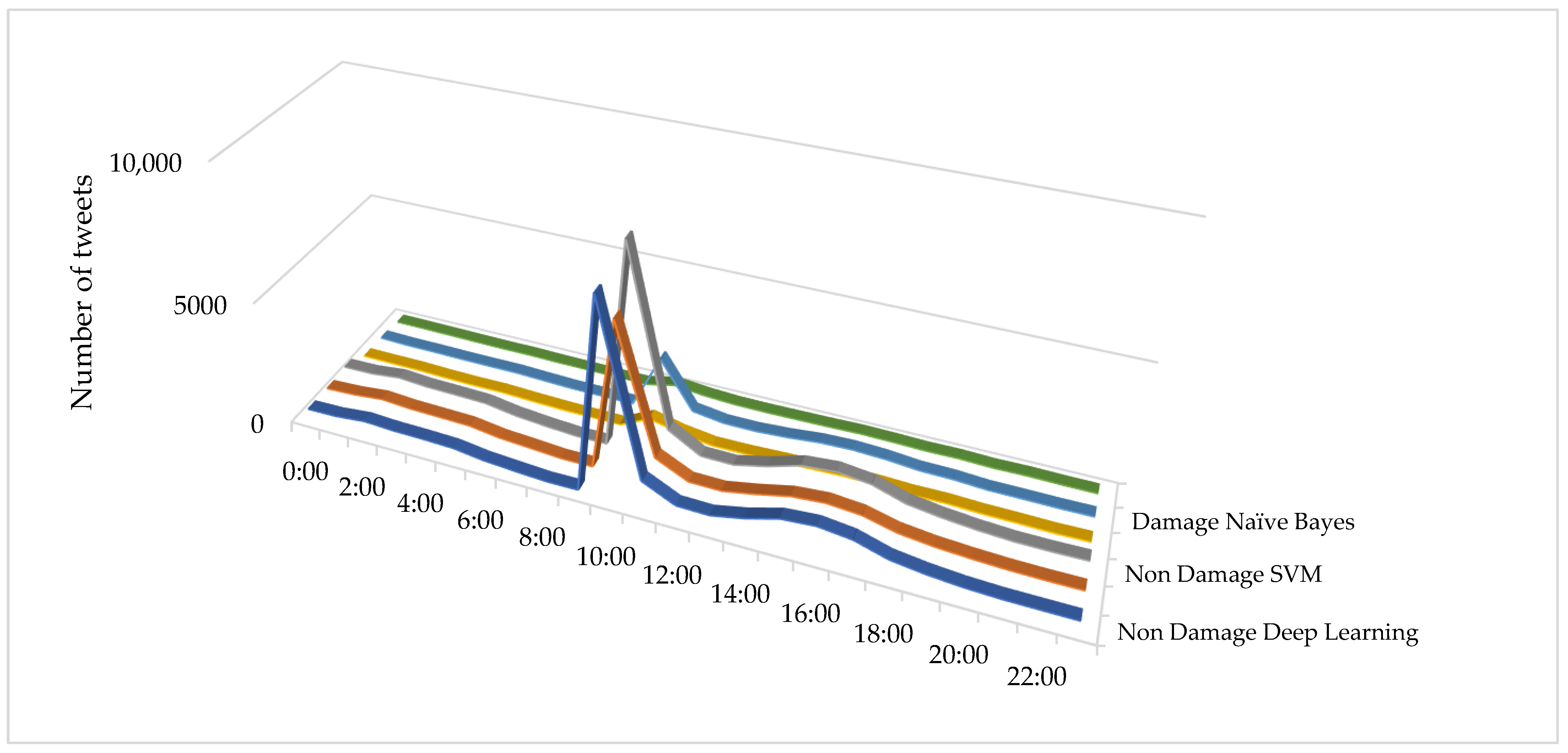
Figure 6 shows the total distribution of classified tweets into the two classes of damage and non-damage at each hour of the earthquake day, by the three Naive Bayes, SVM, and deep learning classification algorithms. In total, 42% (11,293 tweets) of tweets were collected between 9 am and 12 pm. The results of Naive Bayes classification algorithm (
Figure 6) showed that 25.61% of the collected tweets from 9 am to 12 noon (2893 tweets) reported damage, and the rest of the tweets (8403 tweets) reported no damage. In addition, 28.39 percent of the tweets (7630 tweets) were collected between the hours of 14 and 19, of which 24.66 percent (1882 tweets) reported earthquake damage and 5748 tweets reported no damage. The SVM algorithm’s results (
Figure 6) showed that of the 1293 tweets collected between 9 am and 12 noon, 4.77 percent of tweets (539 tweets) reported damage and the rest of the tweets (including 10,757 tweets) reported no damage. In addition, 28.39 percent of tweets (7630 tweets) were collected between the hours of 14 and 19, of which 9.22 percent (704 tweets) reported earthquake damage and 6926 reported no damage. The results of the deep learning algorithm also showed that of the 11,293 tweets collected between 9 am and 12 pm, 10% of tweets (1119 tweets) reported damage, and the rest of the tweets (10,174 tweets) reported no damage. A total of 28.39% of the tweets (7630 tweets) were collected between the hours of 14 and 19, of which 18.6% (1422 tweets) reported earthquake damage and 6208 reported no damage.
In general, all algorithms had a sudden increase in the number of tweets at the time of the earthquake (10 am). There was also another increase in the number of messages at 4 pm, which may be related to the end of office hours and increased activity on social media.
Figure 7 shows the distribution of tweets, classified into five classes, by hour on the day of the earthquake (24 August) for the three—Naive Bayes, SVM, and deep learning—classification algorithms. Examination of the results of Naive Bayes classification algorithm (
Figure 7) showed that most tweets classified between 9 am and 12 pm belonged to the classes “Other_relevant_information” and “Response_efforts” with 79.04% (8929 tweets) and 7.26% (821 tweets), respectively. In addition, tweets for the “Donation”, “Infrastructure”, and “Injured_Dead_and_Missing_people” classes amounted to 6.94% (785 tweets), 5.01% (566 tweets), and 1.72% (195 tweets), respectively. According to SVM algorithm results (
Figure 7), it can be seen that all tweets classified between 9 am and 12 pm belonged to the “Other_relevant_information” class and only one tweet belongs to the “Infrastructure” class. In addition, the deep learning algorithm results (
Figure 7) showed that most tweets classified between 9 am and 12 pm belonged to the classes “Other_relevant_information” and “Injured_Dead_and_Missing_people”, with 33.64% (9041 tweets) and 6.58 percent (1770 tweets), respectively. Additionally the tweets for the “Infrastructure”, “Response_efforts”, and “Donation” classes were 0.98% (265 tweets), 0.67% (182 tweets), and 0.13% (35 tweets) respectively
Figure 7 shows a sudden increase in the number of tweets, at the time of the earthquake (10 am). In addition, the highest increase was for high-urgency classes.
The spatial analysis of social networks could assist us in comprehending the spatial distribution and concentration of emergency topics. For policymakers, this would be helpful for responding to the disaster in a timely manner and with a full understanding of the public concern.
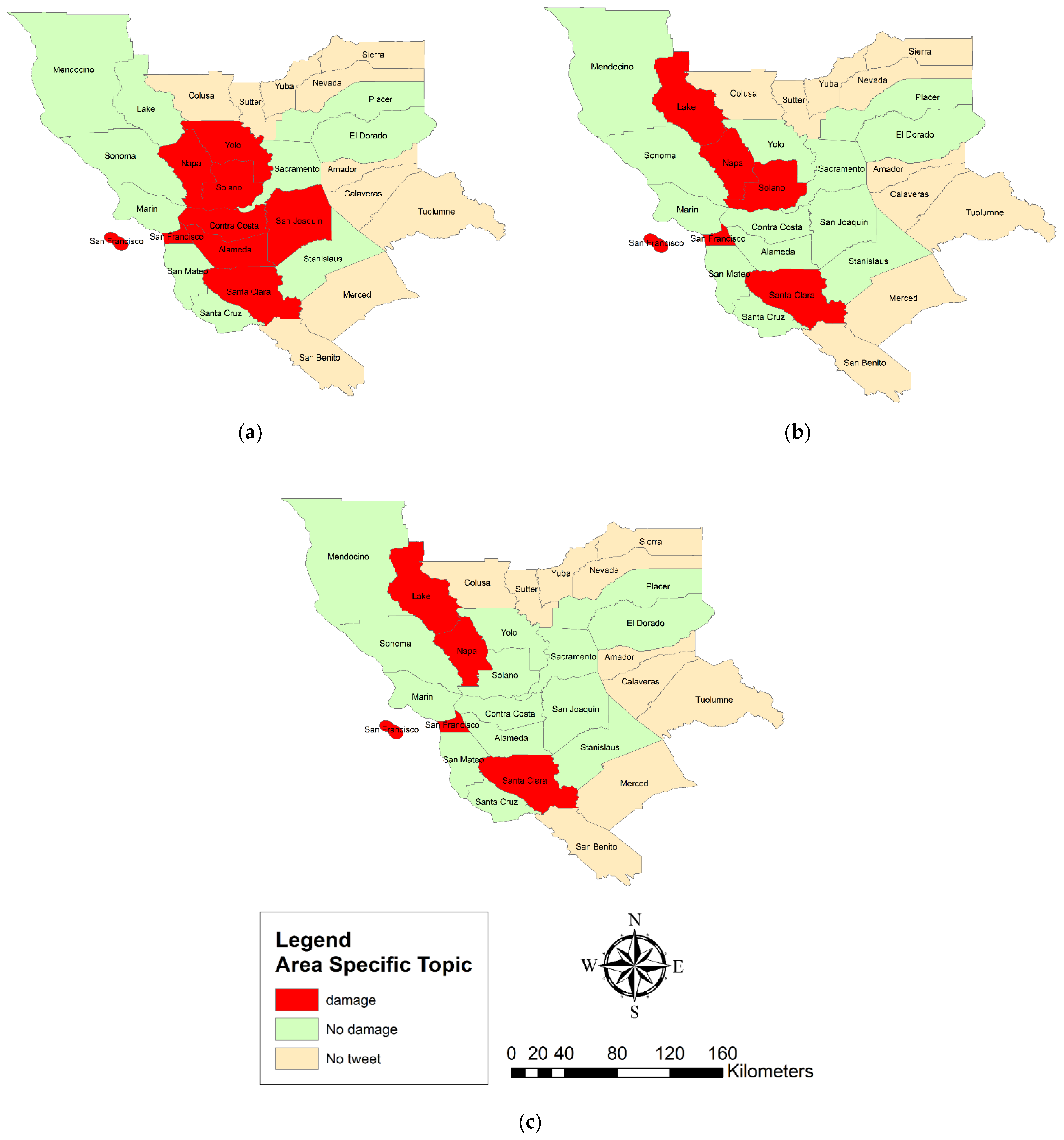
Figure 8 shows the LQ analysis of the tweets’ spatial topic concentration at the county scale, classified by Naive Bayes (a), SVM (b), and deep learning (c) in the two classes of damage and non-damage. According to
Figure 8a, most tweets collected from the counties of Napa, Yolo, Solano, Contra Costa, San Joaquin, San Francisco, Almeda, and Santa Clara showed damage. However, according to
Figure 8b, the results of the SVM algorithm showed that most tweets collected from Napa, Lake, Solano, San Francisco, and Santa Clara counties and other counties reported no damage. In addition, according to the LQ map derived from the deep learning algorithm results (
Figure 8c), most damage tweets were reported in Napa, Lake, San Francisco, and Santa Clara counties.
In all algorithms, Napa, as a center of the earthquake, was considered as having the primary concentration of damage-related messages in all algorithms. This indicates that our approach has been able to identify the damage well and has considered the earthquake center one of the most affected counties. In addition, San Francisco and Santa Clara counties were considered to be damage concentration counties. This may be due to the high urbanization in these two cities, which has led to increased use of social networks and, consequently, more damage-related messages. It is, therefore, suggested that future research consider the effects of urbanization and eliminate its impact on damage estimation.
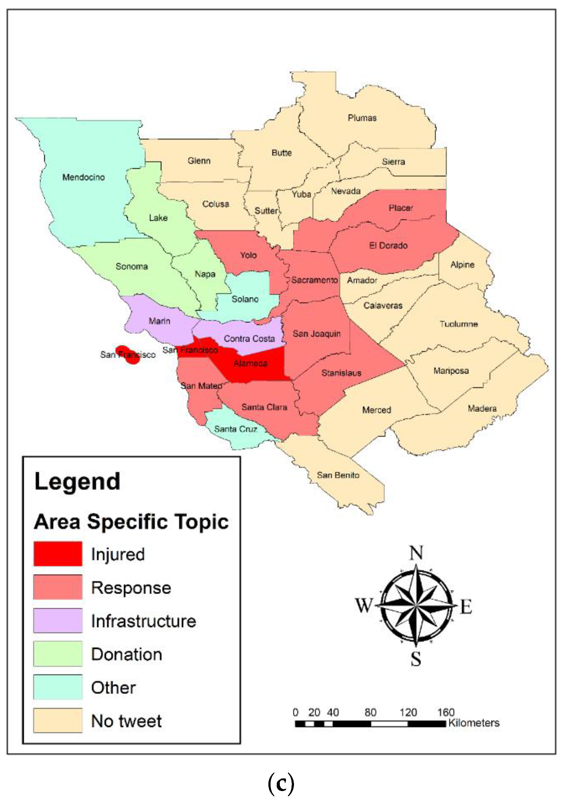
Figure 9 shows the LQ analysis of the tweets’ spatial topic concentration at the county scale, classified by Naive Bayes (a), SVM (b), and deep learning (c) in the two classes of damage and non-damage. According to the results of the Naive Bayes algorithm (
Figure 9a), most of the tweets collected from the Lake, Sonoma, and Santa Clara counties belonged to the “Injured_Dead_and_Missing_people” class, and most of the tweets reported by Marin, Solano, Contra Costa, and Stanislaus were in the “Response_efforts” class. Most of the tweets reported in Napa were of the “Infrastructure” class, and the tweets in Yolo, Almeda, San Francisco, and San Mateo were in the “Donation” class. This indicates that in the center of the earthquake and nearby counties, most of the messages focused on infrastructure damage, injured people, and response, but moving away from the earthquake center, other issues, such as donations, arose.
While according to the LQ map of the SVM algorithm (
Figure 9b), most of the tweets collected in San Francisco and San Mateo belonged to the “Response_efforts label” class, and most of the tweets reported in Napa belonged to the “Infrastructure” class. In other counties, most of the reported tweets belonged to the “Other_relevant_information” class. The LQ map of the deep learning algorithm showed that most of the tweets collected from the Almeda and San Francisco counties belonged to the “Injured_Dead_and_Missing_people” class and most of the tweets reported in Yolo, Placer, El Dorado, Sacramento, San Joaquin, Stanislaus, Santa Clara, and San Mateo belonged to the “Response_efforts” class. In addition, most of the tweets in the Marin and Contra Costa counties were from the “Infrastructure” class, and the Lake, Napa, and Sonoma tweets were from the “Donation” class.
Based on
Figure 9, it can be generally acknowledged that most of the infrastructure damage-related messages focused on Napa County. This indicates that most damages to infrastructure, buildings, and roads occurred in the center of the earthquake.
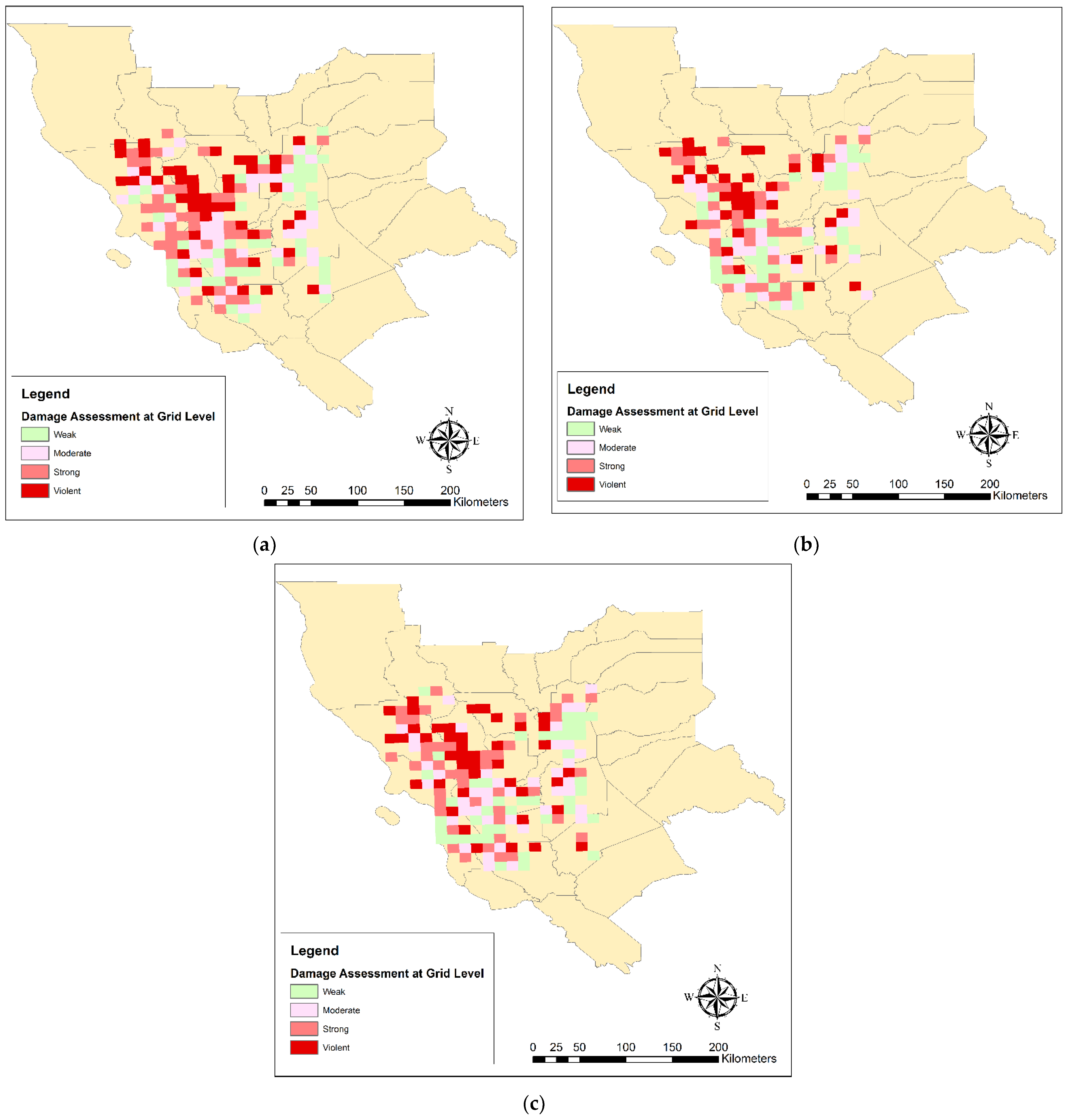
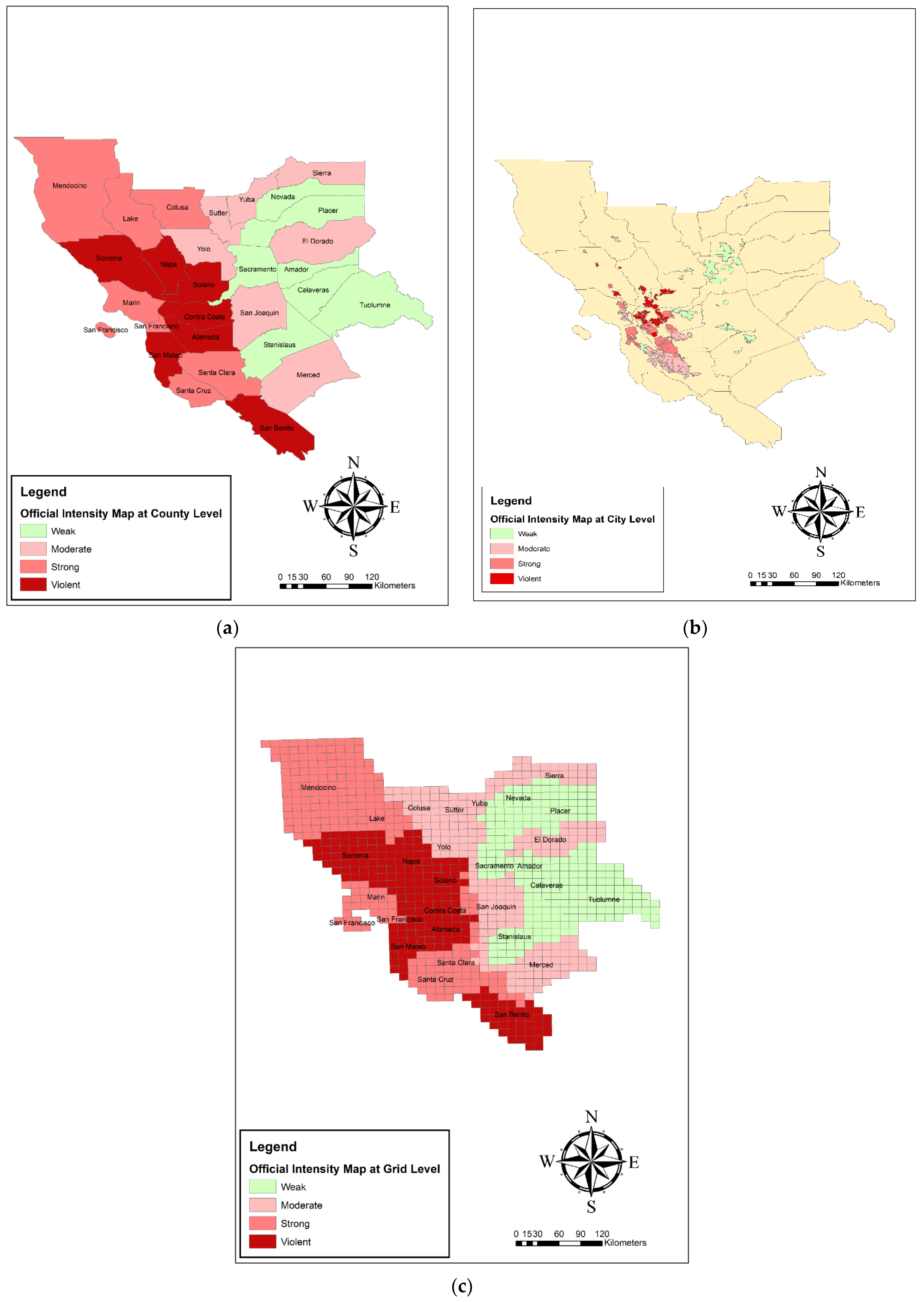
5.4. Damage Validation
In this section, the estimated damage maps from each of the Naive, SVM, and deep learning algorithms were validated using the official damage map at three county, city, and 10 by 10 km grids scales. The official damage map, which was computed based on the FEMA HAZUS loss model, is shown at the three, county, city, and 10 by 10 km grid, scales in
Figure 13.
Table 3 presents the results of the validation of the estimated damage map from Naive Bayes, SVM, and deep learning at the county scale with official data. Based on the validation results by the three indices of Kendall’s tau, Pearson correlation, and Spearman’s rho, the deep learning classifier was selected as the best model at the county scale. In additino, Kendall’s tau and Spearman’s rho indexes, which were used to rank values, performed better than Pearson indices, which worked with the values themselves.
Table 4 presents the results of the validation of the estimated damage map from Naive Bayes, SVM, and deep learning at the city scale with official data. Based on the validation results by the three indices of Kendall’s tau, Pearson correlation, and Spearman’s rho, the SVM classifier was selected as the best model at the city scale.
Table 5 presents the results of the validation of the estimated damage map from Naive Bayes, SVM, and deep learning at the 10 × 10 km grids scale with official data. Based on the validation results by the three indices of Kendall’s tau, Pearson correlation, and Spearman’s rho, the SVM classifier was selected as the best model at the city scale.
Table 6 presents the results of validation of the estimated damage map from Naive Bayes, SVM, and deep learning at the 10 × 10 km raster grids scale with accuracy, precision, recall, and F-score indices. These indices were obtained from the confusion matrix. Based on the validation results by the four indices of accuracy, precision, recall, and F-score, the Naive Bayes classifier was selected as the best model at the 10 × 10 km raster grids.
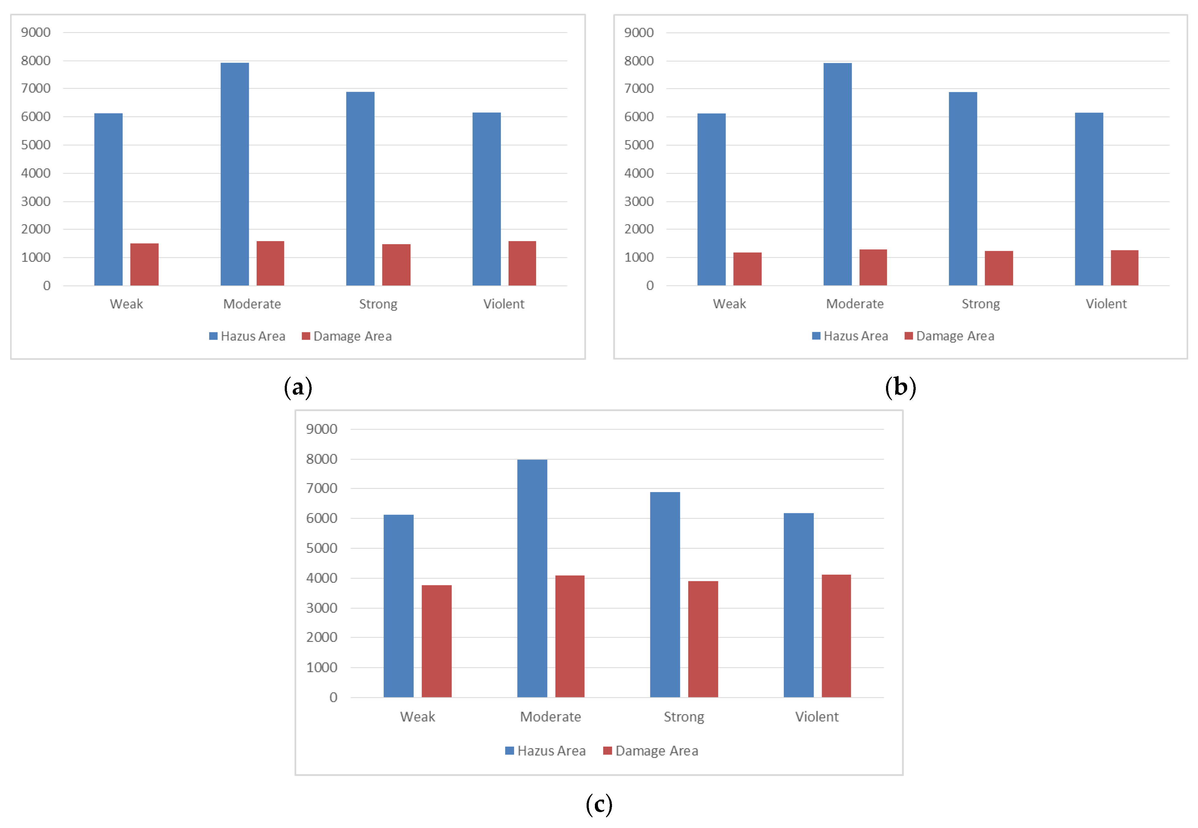
Figure 14 shows the area values (km
2) included by each class in our estimated damage map and FEMA HAZUS loss model map for the Naive Bayes, SVM, and deep learning algorithms. Obviously, the area covered by the four classes in the FEMA HAZUS loss model map for all three algorithms must be equal. In addition, the areas covered by the four classes in the estimated damage map for the two Naive Bayes and SVM algorithms were approximately equal. However, the obtained area corresponded to the results of the four classes in the damage map for the deep learning algorithm, on average 2.8 times more than the same value in the two Naive Bayes and SVM algorithms. In general, the results of the deep learning algorithm in the area covered by four classes were closer to the FEMA HAZUS loss model map (official damage map).
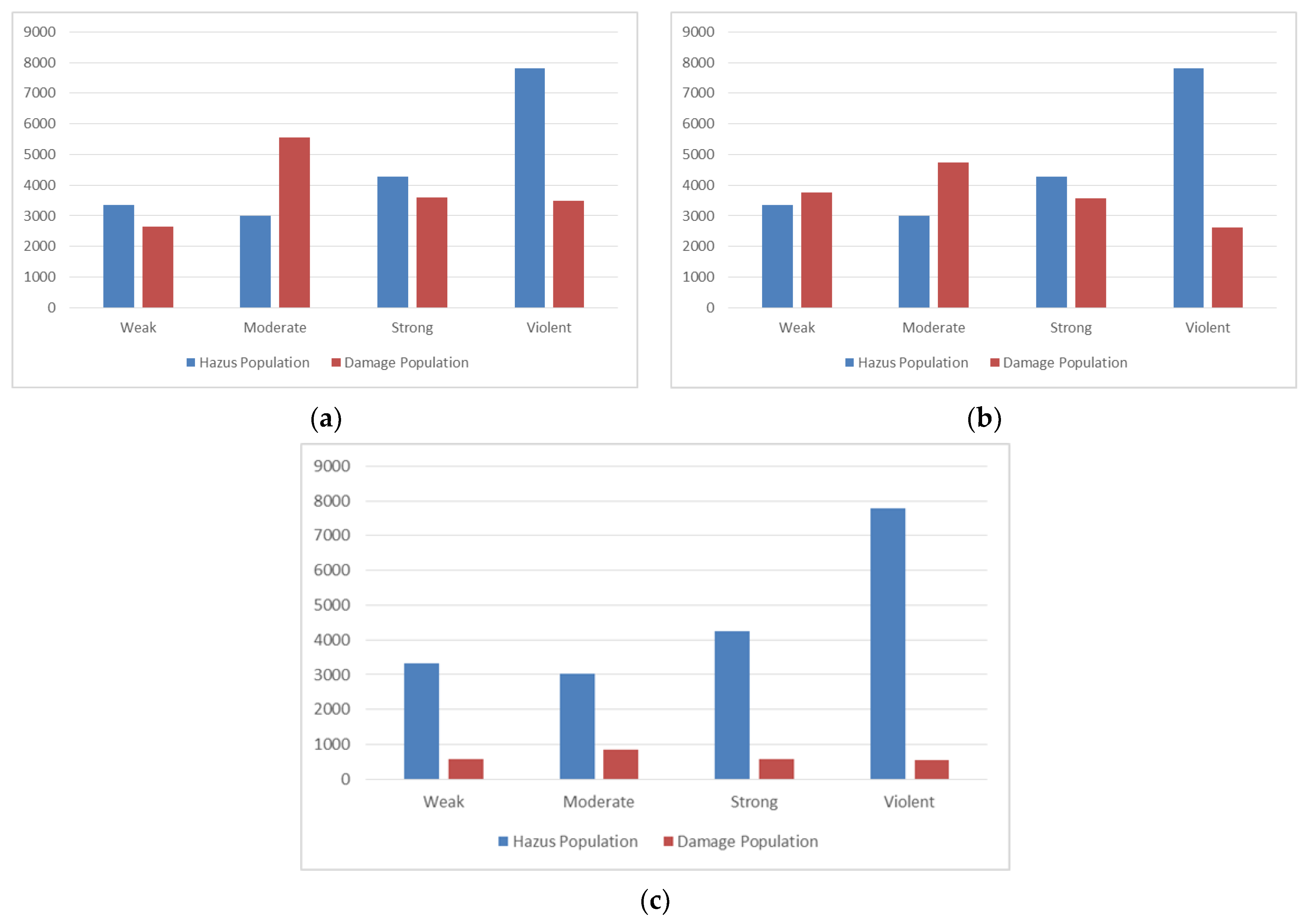
Figure 15 shows the population (in units of a thousand) covered by each class in our estimated damage map and FEMA HAZUS loss model map for the Naive Bayes, SVM, and deep learning algorithms. Obviously, the areas covered by the four classes in the FEMA HAZUS loss model map for all three algorithms must be equal. The populations encompassed by the three classes of weak, strong, and violent were approximately equal in the estimated damage map for the Naive Bayes and SVM algorithms. However, the population size of the moderate class in the Naive Bayes algorithm was almost 800,000 units higher than the similar value in the SVM algorithm.
Additionally, the covered populations corresponded to the results of the four classes in the estimated damage map for the deep learning algorithm, on average 0.18 times lower than the same value in the Naive Bayes and SVM algorithms. In general, the results of the SVM algorithm in the populations covered by three classes of weak, moderate, and strong were closer to the FEMA HAZUS loss model map (official damage map).


