Article

Prediction of Total Imperviousness from Population Density and Land Use Data for Urban Areas (Case Study: South East Queensland, Australia)

School of Engineering and Built Environment, Griffith University, Kessels Road, Nathan, QLD 4111, Australia
*
Author to whom correspondence should be addressed.
Appl. Sci. 2021, 11(21), 10044; https://doi.org/10.3390/app112110044
Submission received: 29 September 2021 / Revised: 23 October 2021 / Accepted: 25 October 2021 / Published: 27 October 2021
(This article belongs to the Section Earth Sciences)

Abstract

:
Total imperviousness (residential and non-residential) increases with population growth in many regions around the world. Population density has been used to predict the total imperviousness in large areas, although population size was only closely related to residential imperviousness. In this study, population density together with land use data for 154 suburbs in Southeast Queensland (SEQ) of Australia were used to develop a new model for total imperviousness estimation. Total imperviousness was extracted through linear spectral mixing analysis (LSMA) using Landsat 8 OLI/TIRS, and then separated into residential and non-residential areas based on land use data for each suburb. Regression models were developed between population density and total imperviousness, and population density and residential imperviousness. Results show that (1) LSMA approach could retrieve imperviousness accurately (RMSE < 10%), (2) linear regression models could be used to estimate both total imperviousness and residential imperviousness better than nonlinear regression models, and (3) correlation between population density and residential imperviousness was higher (R2 = 0.77) than that between population density and total imperviousness (R2 = 0.52); (4) the new model was used to predict the total imperiousness based on population density projections to 2057 for three potential urban development areas in SEQ. This research allows accurate prediction of the total impervious area from population density and service area per capital for other regions in the world.

1. Introduction

South East Queensland (SEQ) is one of the major urban living areas in Australia, in which the population is expected to grow over the next few decades based on government plans. Queensland governments define some centers (new residential suburbs) as potential development areas (PDAs) in the SEQ region (https://www.qld.gov.au/, (accessed on 10 August 2021)). Development of the PDAs will lead to an increase in the total impervious surface area (TISA) including residential buildings and service area, e.g., commercial and industrial services, roads, and parking lots. Total imperviousness (the ratio of TISA to total area) has been shown to be a reliable metric to describe urban development [1]. Several studies explored the destructive impact of the increase in total imperviousness on hydrology and climate condition in urbanized regions [2,3,4,5]. Therefore, accurate estimation of total imperviousness due to population growth in the future is of great importance for developing sustainable environmental management plans.
Census, economic, and geographic data have been known as the main urban growth causative factors [6,7,8,9]. Among them, census data are the most available data which have been recorded every five years in most countries (e.g., Australia) (https://itt.abs.gov.au, (accessed on 15 July 2021)). Additionally, census data have been recorded in large areas such as counties or suburbs [10,11]. On the other hand, urban built-up areas, known as total imperviousness, have been derived at small (e.g., buildings) to regional areas from satellite images [12,13,14]. Imperviousness derived from remote sensing techniques represents total imperviousness (residential and non-residential).
To extract total imperviousness over large areas, previous studies used medium spatial resolution satellite images (e.g., Landsat) [10,11,14,15]. For example, Azar et al. [16] used Landsat images to derive imperviousness at county scale in Haiti. Per-pixel and sub-pixel classification techniques have been used [17,18,19] to extract total imperviousness from Landsat images. Per-pixel methods (e.g., maximum likelihood and support vector machine) based on medium spatial resolution images often overestimate or underestimate total imperviousness, due to presence of mixed pixels especially in urban areas [20]. However, sub-pixel classification approaches such as Artificial Neural Network (ANN) and Spectral Mixture Analysis (SMA) have shown a better performance to quantify the fraction of each land use in each pixel [21,22].
A few simple methods have been used to predict total imperviousness from population density data in large areas [23,24]. Sunde et al. [25] used a coefficient, showing total imperviousness per person, to predict the total imperviousness from population projections. Other studies predicted total imperviousness from population density using established regression models [26,27,28]. Sutton [29] developed a linear regression model between population data and urban area, derived from nighttime satellite imagery, to estimate imperviousness for a large number of urban centers in the United States. Carlson [30] used a nonlinear regression model to predict total imperviousness from population density for two catchments in the US.
The above-mentioned methods have overestimated total imperviousness in dense residential suburbs, where the most of built-up areas are residential buildings. This was mainly because non-residential impervious area is not related to the local population density. Thus, in this study, we aimed to develop a new model to predict the total impervious area in dense residential PDAs in SEQ, Australia. This model could allow us to predict total imperviousness in urban development areas in Australia and other areas in the world with higher accuracy. The specific objectives of this study were to address the following research questions:
  • Whether or not a sub-pixel classification approach can extract imperviousness with acceptable accuracy in our case study, which is a complex urban–rural frontier.
  • What is the nature of the relationship, linear or nonlinear, between population density and total imperviousness, and between population density and the residential impervious at the suburb scale?
  • Whether or not population density is a better predictor of residential imperviousness than total imperviousness at suburb scale?
  • Whether or not our recommended method could be used to estimate total imperviousness more accurately than previous regression models between population density and total imperviousness in dense residential suburbs?

2. Material and Methods
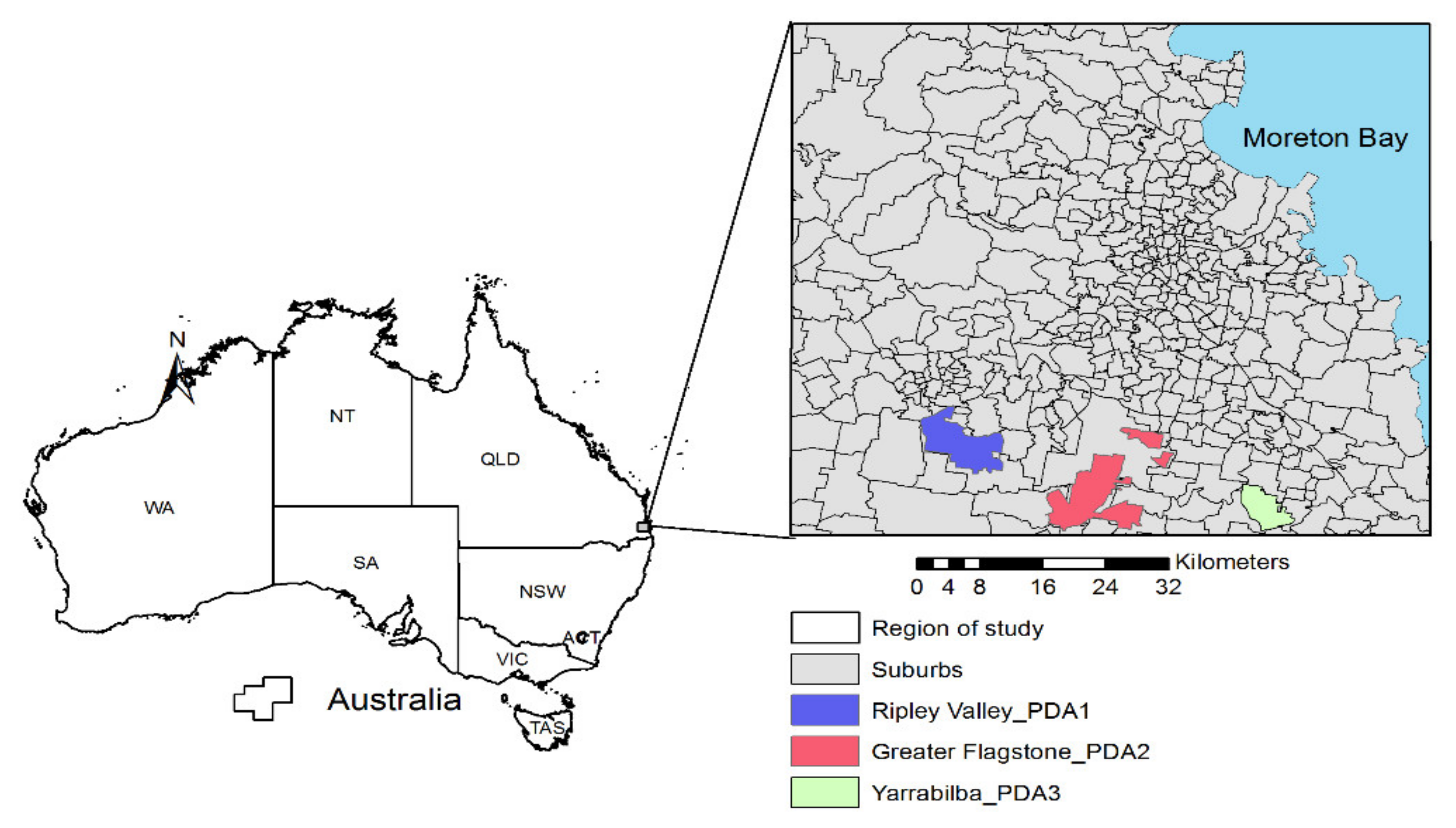
2.1. Study Area

The study area consists of more than 310 suburbs, located in South East Queensland, Australia (Figure 1). SEQ contains major urbanized areas such as Brisbane, Logan, and Ipswich cities in with a population of around 3.5 million people in 2016. Based on population growth projections, potential development areas (PDAs) were defined in SEQ region (https://www.qld.gov.au/, (accessed on 10 August 2021)). Ripley Valley (46 km2), Greater Flagstone (72 km2), and Yarrabilba (22 km2) are three largest PDAs in Queensland. These PDAs are located in one of the largest urban growth areas in Australia (Figure 1). They offer opportunities for further residential growth to meet the region’s affordable housing needs. Once the area is fully developed, Ripley Valley, Greater Flagstone, and Yarrabilba are expected to have a population of 120, 120, and 50 thousand people, respectively, by 2060.

2.2. Dataset

Landsat images (TM, ETM and OLI/TIRS), as a medium resolution image, were used widely to derive imperviousness in environmental studies [31,32,33,34,35,36]. Hence, Landsat 8 OLI/TIRS image (collection 1 Level-2) which provides surface reflectance data (path/row: 89/79) in July 2016 was used in this study (https://earthexplorer.usgs.gov/, (accessed on 20 October 2021)). Cloud-free Landsat 8 OLI/TIRS images and that with minimal system-induced errors such as stripping or bad pixels which have higher quality rate for image analysis purposes were selected. No atmospheric correction and no image to image registration were needed because Level-2 Surface Reflectance data are atmospherically and geometrically corrected. High resolution and cloud-free Google Earth images in July 2016 were used to obtain imperviousness data for evaluating the accuracy of Landsat-derived imperviousness data. Population data at the suburb scale was obtained from Australian Bureau of statistics (https://itt.abs.gov.au/, (accessed on 15 July 2021)). Population data were available for 154 suburbs for the year 2016. Therefore, 154 suburbs from a total of 310 suburbs were selected for this study. Area of the selected suburbs was obtained from polygon layer of suburbs provided by the Australian Government website (https://data.gov.au/, (accessed on 10 August 2021)). Residential polygons were derived from SEQ land use map in 2015.

2.3. Extraction of Total Imperviousness

Two main steps were used in this research to derive imperviousness from Landsat 8 OLI/TIRS.
  • Step 1: Removal of water bodies
Modified Normalized Difference Water Index (MNDWI) (Equation (1)), as a widely used satellite-derived index, was used to remove water pixels from Landsat images [37].
MNDWI = R Green - R SWIR 1 R Green + R SWIR 1
where, RGreen and RSWIR1 refer to Landsat 8 OLI/TIRS surface reflectance values of consistent bands Green (band 3) and SWIR1 (band 6). MNWDI is a good indicator of liquid water and less sensitive to atmosphere that has been widely used in environmental research [38,39,40,41]. With MNWDI, those pixels with a threshold value of greater than 0 were represented as water bodies and masked from the image.
  • Step 2: Sub-pixel classification approach
The linear spectral mixture analysis (LSMA)-based method was applied in this study to extract total imperviousness from Landsat images [42]. The LSMA approach assumes that the surface reflectance measured by a sensor in each band is a linear combination of the surface reflectance of end members (each end member represents a pure land cover type) within the pixel and that the surface reflectance proportions of the end members represent proportions of the area covered by distinct features on the ground. The linear spectral mixing model is expressed as:
R j = i = 1 N f i R ij + e j
i = 1 N f i = 1
where Rj is the surface reflectance for each band (j) in the Landsat 8 OLI/TIRS image (6 bands), N is the number of end members, fi is the fraction of end member i, Rij is the surface reflectance by the end member i in band j, and ej is the unmodeled residual. Six Landsat 8 OLI/TIRS reflective bands (Visible, NIIR, and SWIR bands) were used to develop fraction images with LSMA. Additionally, constrained condition was imposed based on Equation (3) which means the sum of all fractions must equal 1. Moreover, four endmembers including vegetation, low-albedo (e.g., dark impervious surface materials), high-albedo (e.g., commercial/industrial/transportation areas), and soil, were selected as input to LSMA in this study. Total imperviousness in each pixel was extracted from the sum of high-albedo and low-albedo fraction images [43,44] (Figure 2). A detailed description of the LSMA method, selected Landsat reflective bands, and end-member selection were found in previous literature [34,45]. In order to assess the accuracy of extracted imperviousness map, 300 random samples (each sample contains 3 × 3 Landsat pixels) were initially selected over the Landsat imperviousness map. Samples were selected over the whole study area with different degrees of urbanization (0 to 100%). This stratified sampling method allowed us to check the performance of the LSMA algorithm for a wide range of imperviousness in the study area. The selected samples over Landsat images were linked to the corresponding Google Earth image. Impervious areas were digitized manually for each sample in the Google Earth image [46,47]. The impervious areas were then divided by the total sample area to calculate imperviousness in percent for each sample. Both Landsat and Google earth images had similar acquisition dates (June of 2016) that reduce errors related to land use change in the validation process. Values of imperviousness derived from Landsat and Google Earth were compared by widely used statistical criteria including the coefficient of determination (R2), the root mean square error (RMSE), and the mean absolute error (MAE).

2.4. Relatioship between Population Density and Total Imperviousness

Total imperviousness derived from the LSMA approach at Landsat pixel was aggregated for each suburb (Figure 2). Among around 250 suburbs, 154 suburbs, where population density data are available, were selected for further analysis. Total imperviousness (%) and population density (persons/km2) for each suburb were used as dependent variable and independent variable, respectively. Linear and nonlinear regression models were developed. Performance of the regression models was assessed by the coefficient of determination (R2), mean absolute error (MAE), and root mean square error (RMSE).

2.5. Model Development between Population Density and Residential Imperviousness

Residential polygon boundary of the land use map (Figure 3), which involves residential building, footpath, and street, was used to separate residential imperviousness. Residential and non-residential imperviousness are shown in Figure 3. Subsequently, residential imperviousness and non-residential imperviousness in each suburb were calculated (Figure 3).
Linear and nonlinear regression models were established between the population density (the independent variable) and residential imperviousness (dependent variable). Similar to Section 2.4, R2, MAE, and RMSE were used to find the best regression model.

2.6. Estimation of the Total Imperviousness Dense Residential Suburbs

Two methods were used to estimate total imperviousness in dense residential suburbs in this study. For this purpose, 67 suburbs with residential imperviousness more than 70% were selected. In method 1, the best relationship between population density and total imperviousness (see Section 2.4) was used. In method 2, residential imperviousness was predicted from population density using the best regression model explained in Section 2.5. Non-residential imperviousness was also predicted using the following steps:
First, to prevent overestimation of non-residential imperviousness, a ratio (M) showing non-residential impervious area per person in the 67 dense residential suburbs, with more than 70% residential imperviousness, was calculated (Equation (4)).
M = 1 N ISA c 1 N P
where, ISAc, P, and N are non-residential impervious areas, population, and number of dense residential suburbs, respectively.
Second, non-residential imperviousness (Ic) for each suburb was computed using Equation (5):
I c = M P A
where P is the population and A the area of each suburb.
Total imperviousness was calculated by aggregating non-residential imperviousness (Ic) and residential imperviousness (Ir) (Equation (6)) for the suburbs:
I = I r + I c
Ultimately, estimated total imperviousness by the two methods were assessed by some commonly used statistical criteria, e.g., RMSE and MAE.

3. Results

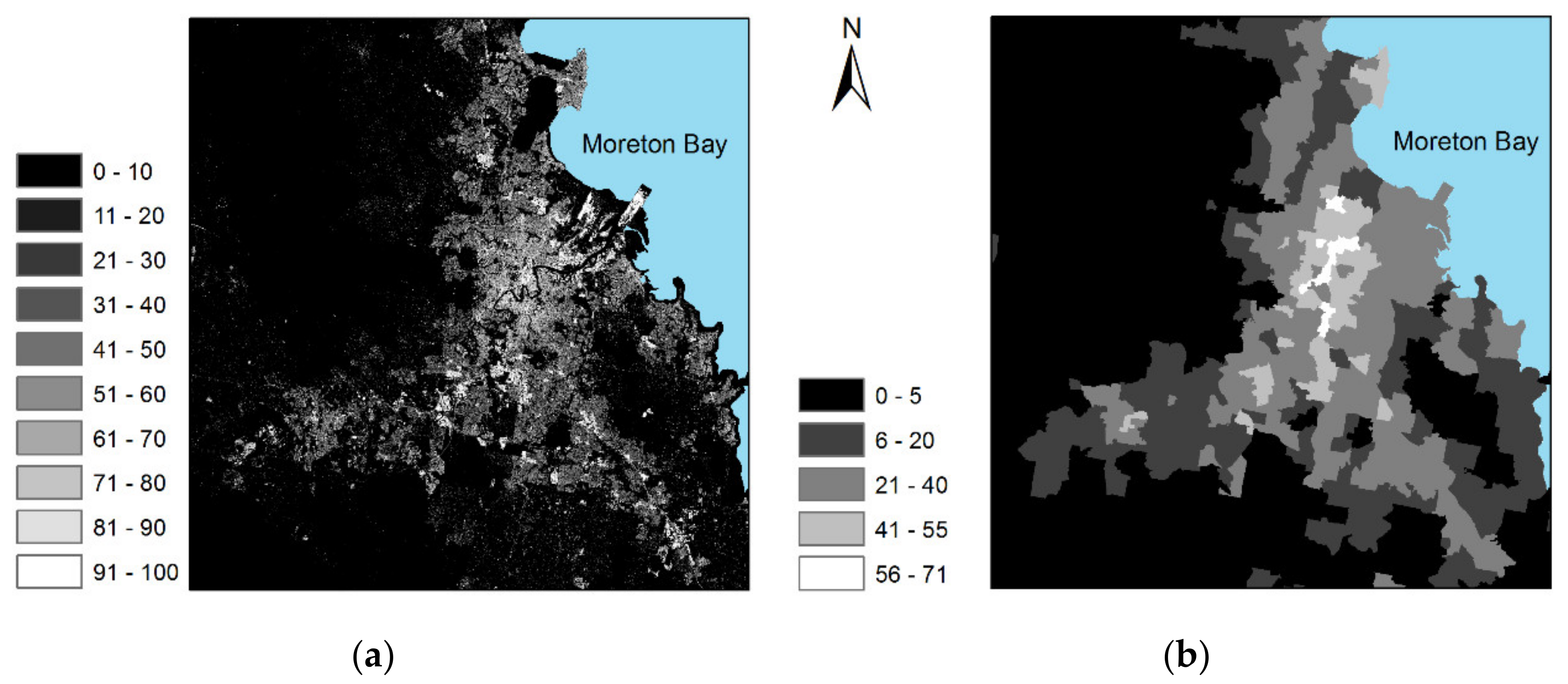
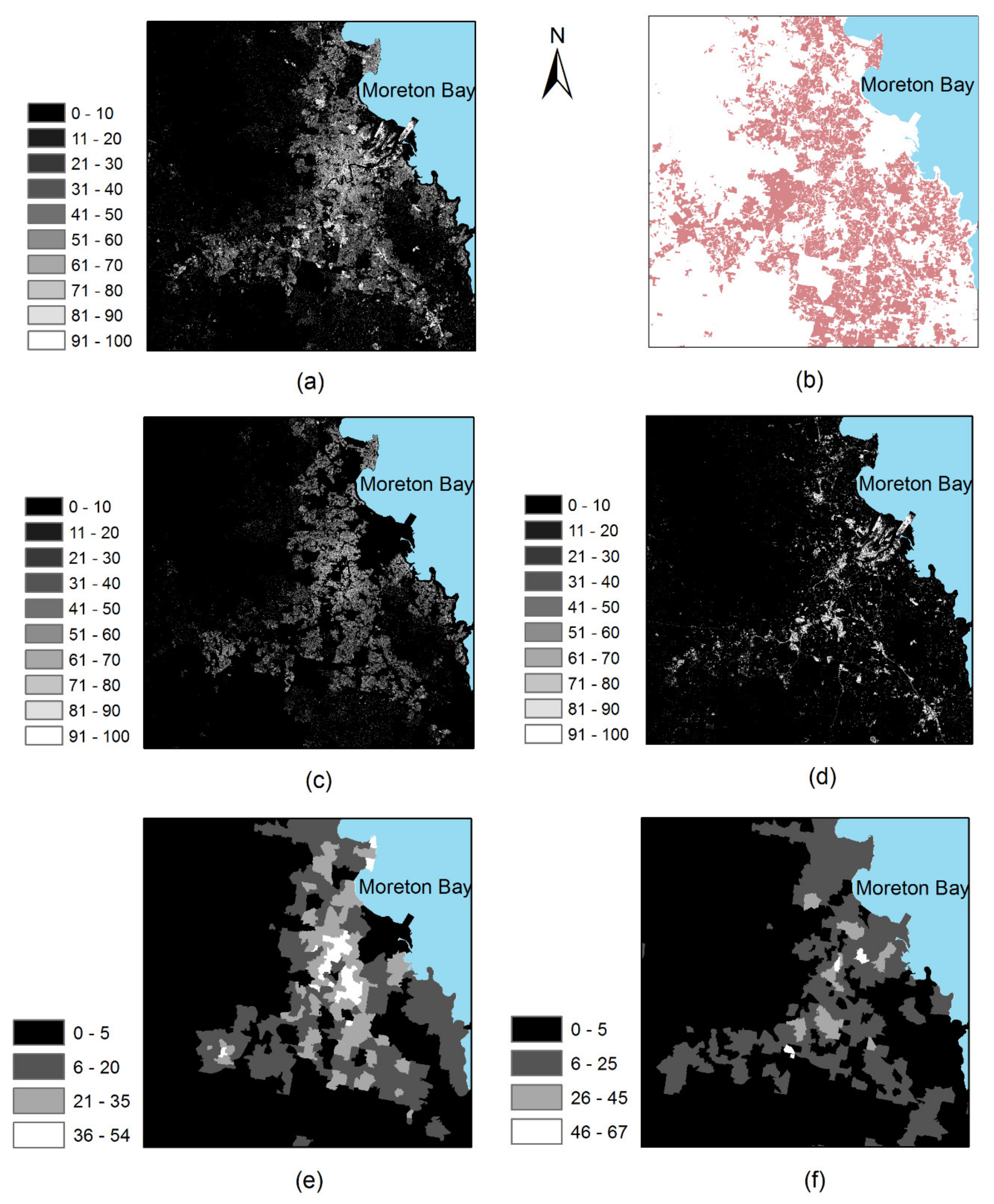
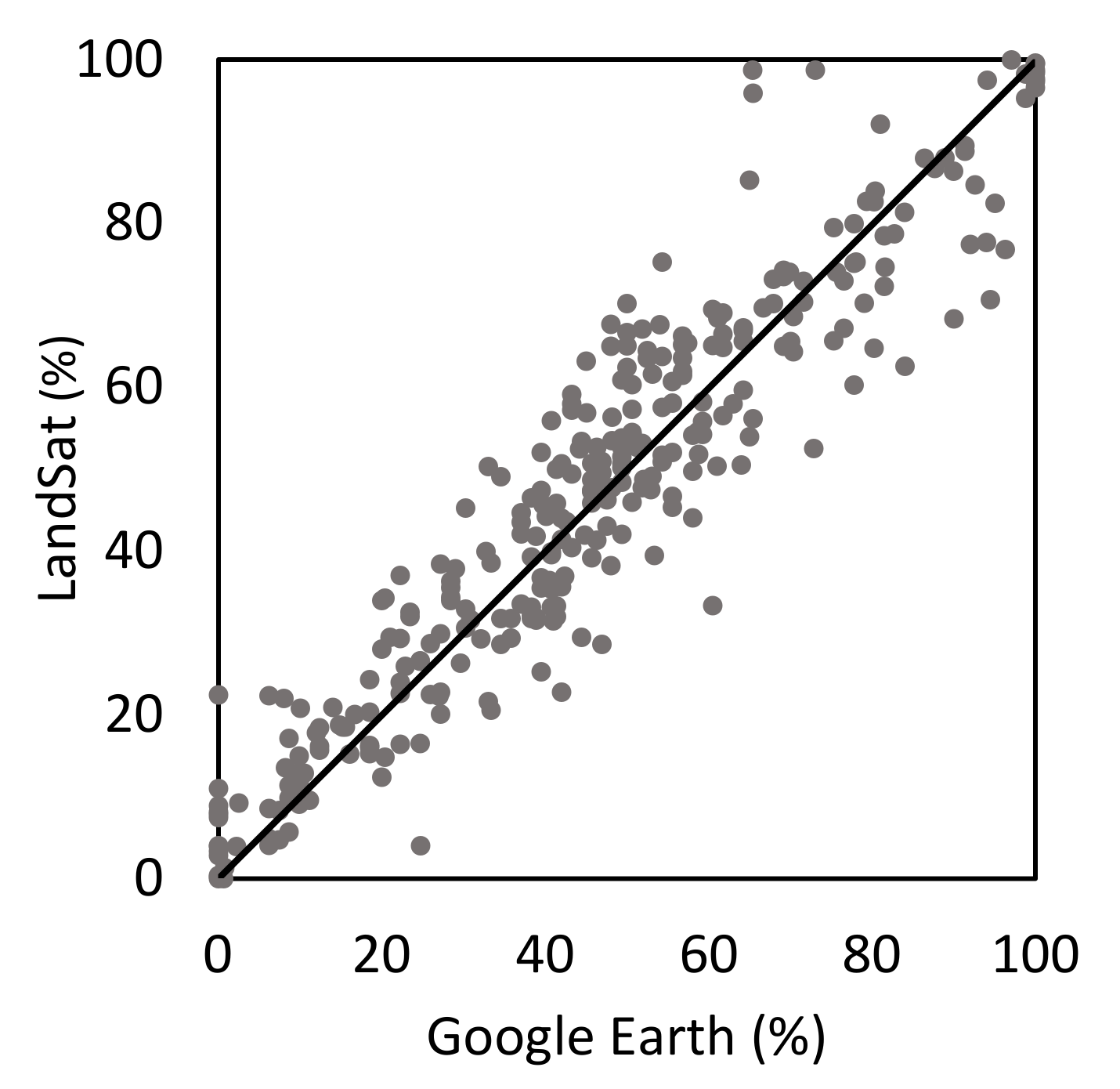
3.1. Evaluation of Extracted Total Imperviousness

Landsat derived imperviousness by LSMA approach was compared to corresponding Google Earth data (Figure 4) in 300 samples. Results showed good agreement between the estimated and the observed data (Figure 4) with a determination coefficient (R2) of 0.87. RMSE of 9% and MAE of 7% also demonstrated a reliable accuracy for imperviousness estimated from Landsat 8 OLI/TIRS by the fully constrained LSMA approach in this study. The LSMA approach, however, overestimated and underestimated imperviousness in samples with imperviousness less than 20% and higher than 80% (Figure 4).
Overestimation mainly occurs in samples with a high fraction of bare soil. This is mainly because bare soil is so similar to some impervious surface materials in terms of spectral behavior [34]. Evaluation indicators from this study were comparable with previous results (Table 1). For example, RMSE from this study is equal to or better than previous results [48,49]. Moreover, MAE is lower than that from study conducted by Li and Lu [10] and Van de Voorde et al. [50]. This comparison indicates that the magnitude of the error is acceptable for this case study (SEQ region) which is a complex urban–rural frontier in Australia.

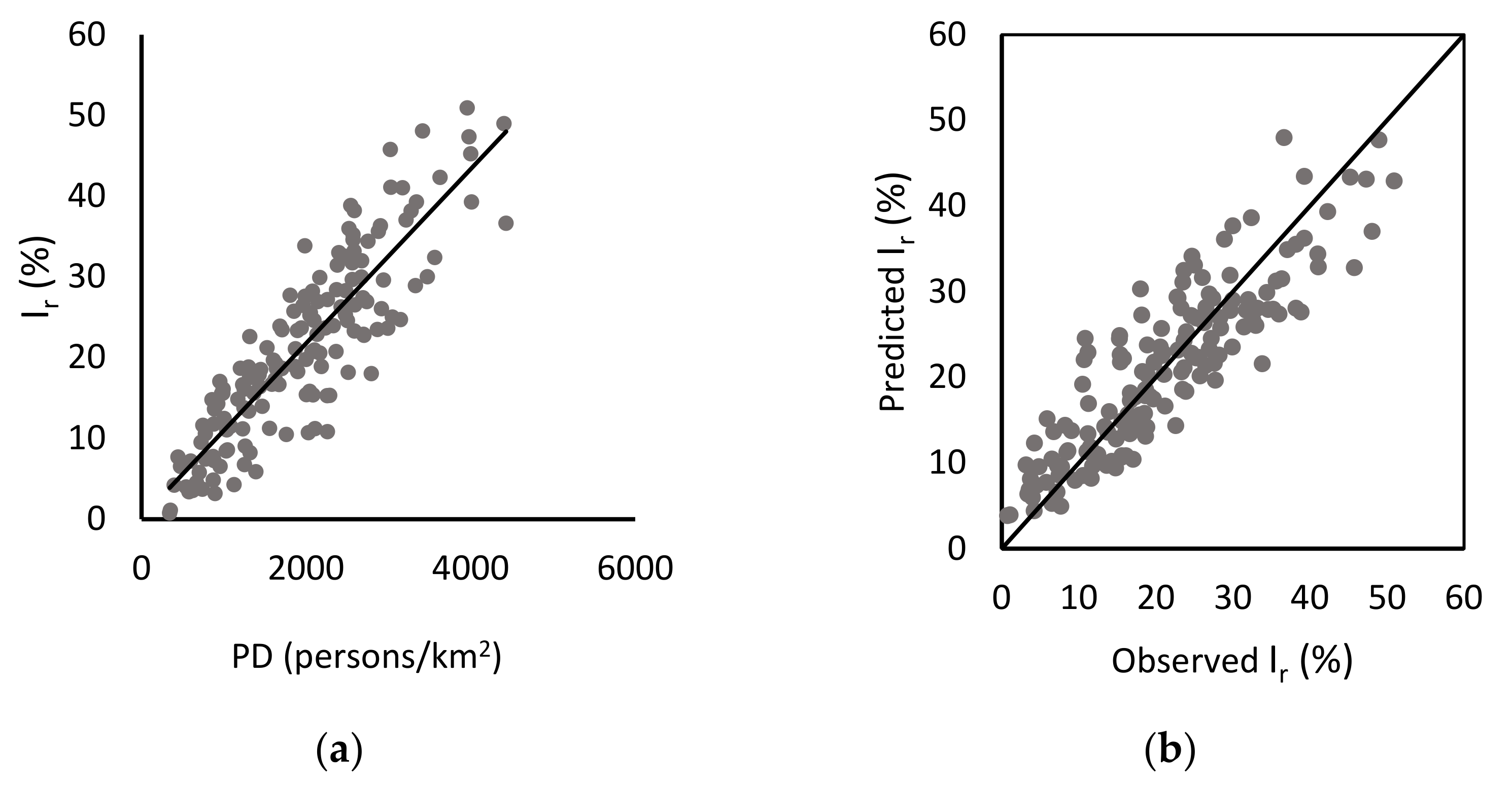
3.2. Relationship between the Total Imperviousness and Population Density

Total imperviousness and population density values for the 154 selected suburbs ranged from 5% to 62%, and 343 to 4430 (persons/km2) in this study. The data range in this study was larger than that (total imperviousness: 1–24% and population density: 70–950 persons/km2) in recent previous studies over large areas (county scale) in China [10]. Different linear and nonlinear regression models were created between population density (PD) and total imperviousness (TI) (Table 2). Capability of the models was assessed using three criteria of R2, MAE, and RMSE. Among them, the linear regression model showed the highest accuracy with determination of coefficient (R2), mean absolute error (MAE), and root mean absolute error (RMSE) of 0.52, 6.77, and 9.06, respectively. Power regression also showed good accuracy compared to the linear regression. The values for the three criteria are approximately similar to corresponding values from the linear model. Other regression models (exponential and logarithmic) demonstrated lower accuracy. Totally, the linear model can more accurately represent the relationship between population density and total imperviousness at suburb scale than nonlinear models in this study (Figure 5). Predicted total imperviousness for the 154 suburbs by the linear regression model versus observed data is shown in Figure 5.
This result is corresponding to the result shown by Azar et al. [16]. They also demonstrated that the linear regression model is the best model to explore the relationship between population density and total imperviousness compared to the nonlinear regressions over a large area. However, Li and Lu [10] indicated that their relationship can be expressed with an exponential equation. In comparison with this study, Azar et al. [16] and Li and Lu [10] showed a stronger relationship between population density and total imperviousness with R2 of 0.85 and 0.88, respectively. Both of these previous studies, however, have developed regression models between the population density and total imperviousness at a scale much larger than that in this study. For example, Li and Lu [10] developed the regression model at the county scale (>1000 km2) in China, which was significantly larger than the suburb scale (1–26 km2) considered in this study.
The relationship between population density and total imperviousness in this study is poor because there are some significant outliers in data. As shown in Figure 5, there are some outliers which refer to suburbs with low population density and high total imperviousness. It is found that they are mostly associated with suburbs where non-residential imperviousness (e.g., industrial areas, shopping areas and public services) is a significant component of the total imperviousness. For example, three of the outliers shown by red color are suburbs with imperviousness of more than 80%. In contrast, two of the outliers shown by blue color are suburbs with residential imperviousness of more than 90%.

3.3. Relationship between the Population Density and Residential Imperviousness

The range of residential imperviousness and population density used in this study is within 0.7–51% and 365–4762 persons/km2. Linear and three nonlinear regression models were developed between population density (PD) and residential imperviousness (Ir) (Table 1). Based on R2, MAE, and RMSE, residential imperviousness in the 154 suburbs can be estimated with a higher accuracy by linear regression model than power regression model. Therefore, the linear regression model which leads to lower error is selected as the best model in this study (Figure 6). Exponential and logarithmic models, however, significantly estimate the residential imperviousness with lower correlation and accuracy compared to the linear and power models. Figure 6 also shows predicted residential imperviousness by the best model and observed data.
Results reveal a stronger relationship between population density and residential imperviousness than that between the population density and total imperviousness (Figure 5 and Figure 6). This is mainly owing to removal of important non-residential impervious areas such as service buildings (hospitals, universities, shopping centers), industrial areas, and major highways in each suburb. If the current land use map could separate other non-residential impervious areas such as streets and pedestrian pathways, a stronger model than the recent linear regression model (Table 3) can be developed. In this model, errors related to building structures are the major source of error which reduces accuracy of the developed model between population density and residential imperviousness. Having said that, information about height of building, as an important characteristic of building structure at suburb scale, is not available in this study.

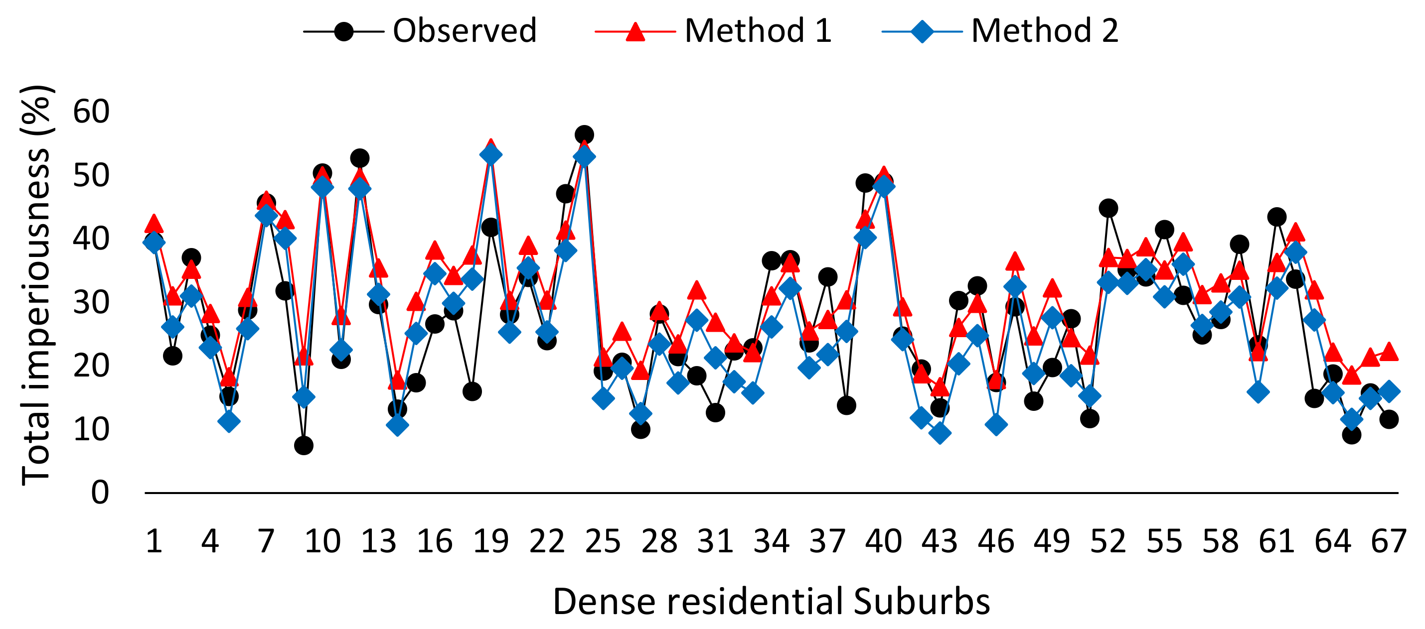
3.4. Accuracy Assessment of the Two Methods for Dense Residential Suburbs

Non-residential impervious area per person (M) for the 67 suburbs was equal to approximately 12 m2. As mentioned in Section 2.6, total imperviousness from the two methods was estimated and compared. RMSE and MAE between observed and estimated total imperviousness derived from method 1 and method 2 was approximately 7.2 and 6.2, and 6 and 5, respectively. It is demonstrated that our recommended method (method 2) had a better overall accuracy than method 1 to estimate total imperviousness in 67 dense residential suburbs in the SEQ.
Figure 7 shows observed total imperviousness and its corresponding predicted values derived from the two methods for each dense residential suburb. Compare to method 2, method 1 overestimated total imperviousness in most of the dense residential suburbs. Additionally, in suburbs that both of the methods show overestimation, method 2 predicted lower overestimation than method 1. Moreover, analyzing the results revealed that average of total imperviousness in all suburbs was overestimated by up to 15% by method 1; however, near 2.5% underestimation was observed using method 2. It demonstrates the overall overestimation of total imperviousness in the 67 dense residential suburbs predicted from method 1 compared to method 2 in this case study.

3.5. Prediction of Total Imperviousness for New Urban Regions in 2057

Method 2, as the more accurate method than method 1, was used to predict total imperviousness in this study. Population density projections in 2057 for three potential development areas (PDAs) were used to predict residential imperviousness by the linear regression model (Table 3). Residential imperviousness, as the main part of development in the PDAS, is expected to occupy 28.3%, 18.2%, and 24.7% area of Ripley Valley, Greater Flagstone, and Yarrabilba. Moreover, according to the non-residential impervious area per person (M = 12 m2), non-residential imperviousness is expected to be approximately 3.1%, 2%, and 2.7% in the PDAs (Table 4). Totally, this study predicted that total imperviousness would be around 31.4%, 20.2%, and 27.4% for the three PDAs. Results showed that more than 20% of area of the PDAs would be replaced with impervious surface area (ISA) in the future. Therefore, sustainable environmental management decisions should be taken to reduce adverse effects of the expected increase in the imperviousness on the ecosystem of these regions.
Here, some sources of uncertainty which may affect the reliability of the predicted total imperviousness are discussed. First, there is uncertainty in the predicted residential imperviousness using the linear regression model (Table 3). The 95% confidence intervals were calculated to show the uncertainty interval for the predicted residential imperviousness. Detailed description to calculate 95% confidence interval for predicted values from regression models was discussed in, e.g., Bewick et al. [51]. The 95% confidence interval was predicted to range from 3.6% to 3.7% for the three PDAs (Table 4). Considering these prediction intervals, a range of total imperviousness for the three PDAs are presented in Table 4. For example, total imperviousness in the Yarrabilba was predicted to range from 23.8% to 31%. Second, uncertainty in population projections was yet another source of uncertainty in the predicted total imperviousness for the PDAs. While, it is difficult to quantify the uncertainty in estimates of population increases. Simple analysis showed how sensitive the predicted imperviousness could be to population projection uncertainties. For example, a 10% increase in population projection would lead to increase in the impervious area between 2% and 3.1% for the three PDAs. The last source of uncertainty source is related to the M ratio which was used to estimate non-residential imperviousness in the PDAs. Analysis showed that there is 45 m2 of non-residential area per person in all 154 suburbs, because non-residential area in some of the suburbs was extremely high. Considering 45 m2 would lead to overestimation of non-residential area, thus, our recommended method could present a low uncertain level of non-residential area for the predicted non-residential imperviousness in the PDAs. Due to the increased land value and population density, our estimate is likely to be the upper limit based on established dense residential suburbs in SEQ.

4. Discussion

In reality, population density is mostly available in large areas such as counties in China [10] and suburbs in Australia. On the other hand, imperviousness can be accurately derived at the corresponding scale with population density (large area) by several advanced sub-pixel classification techniques such as linear spectral mixture analysis (LSMA) or neural network [17,21] from high to medium resolution satellite images, e.g., Landsat [16]. However, this imperviousness represents total imperviousness involving residential imperviousness and non-residential imperviousness. Residential imperviousness simply refers to residential buildings where people live. Non-residential imperviousness encompasses industrial areas, commercial buildings, or transportation infrastructures. Both residential and non-residential impervious areas have different characteristics in terms of their relationship to population size. For example, for a high non-residential suburb (e.g., industrial suburb), where population density is often low, total imperviousness estimation is seriously underestimated based on population density alone and vice versa.
This indicates the importance of estimating residential and non-residential imperviousness separately by taking land use types into consideration. However, satellite-derived imperviousness cannot directly be separated without incorporating land use data [43]. Due to the lack of land use data, underestimation and overestimation of total imperviousness is common for non-residential regions where high total imperviousness exists and for residential areas where low total imperviousness exists [52]. Therefore, considering land use data is of great importance to develop separate residential and non-residential imperviousness estimation models.
In an urbanized region, another important factor resulting in different patterns of total imperviousness is building height. For highly populated areas, suburbs with multi-story (tall) buildings, overestimation of population density is common [52,53]. To address this problem, Lidar data which provide data on height of buildings (structure of buildings) could be used in the future studies to test whether or not relationships between population density and residential imperviousness could be improved at suburb scale.

5. Conclusions

This paper provides a new approach to predict total imperviousness for residential suburbs, based on the established relationship between population density and remote-sensing-derived residential imperviousness and a value (M) representing overall non-residential area per person at the suburb scale. It is concluded that (1) the LSMA sub-pixel classification approach had an overall good accuracy to retrieve total imperviousness in this case study, (2) linear regression models could reproduce both total and residential imperviousness by population density at suburb scale, (3) there was a stronger relationship between population density and residential imperviousness than that between total imperviousness at suburb scale, and (4) the proposed method provided a more accurate and reliable model to predict total imperviousness in 67 dense residential suburbs in Southeast Queensland, Australia. The proposed method is especially valuable for regions where new suburbs would be developed to meet growing need for homes (house buildings). Although this research demonstrated that residential imperviousness could be predicted more accurately by population density, errors related to structure of buildings (heights of the buildings) led to uncertainty in the established model. More research is needed in the future to integrate heights of the buildings into remote-sensing data to develop a more reliable residential imperviousness estimation model.

Author Contributions

All authors contributed significantly to the preparation of this manuscript. Conceptualization, B.Y. and M.R.R.; methodology, M.R.R., B.Y. and Y.C.; software, M.R.R. and Y.C.; data curation, M.R.R. and B.Y.; writing—original draft preparation, M.R.R. and B.Y.; writing—review and editing, M.R.R., B.Y. and Y.C.; visualization, M.R.R.; supervision, B.Y.; project administration, B.Y. All authors have read and agreed to the published version of the manuscript.

Funding

This research received no external funding.

Institutional Review Board Statement

Not applicable.

Informed Consent Statement

Not applicable.

Data Availability Statement

All data used in this article are public record. The links are provided in the text.

Acknowledgments

The authors acknowledge Griffith University, Queensland, Australia for providing financial support through GUIPRS and GUPRS scholarships.

Conflicts of Interest

The authors declare no conflict of interest.

References

  1. Arnold, C.L., Jr.; Gibbons, C.J. Impervious surface coverage: The emergence of a key environmental indicator. J. Am. Plan. Assoc. 1996, 62, 243–258. [Google Scholar] [CrossRef]
  2. Li, C.; Liu, M.; Hu, Y.; Shi, T.; Qu, X.; Walter, M.T. Effects of urbanization on direct runoff characteristics in urban functional zones. Sci. Total Environ. 2018, 643, 301–311. [Google Scholar] [CrossRef] [PubMed]
  3. Morabito, M.; Crisci, A.; Georgiadis, T.; Orlandini, S.; Munafò, M.; Congedo, L.; Rota, P.; Zazzi, M. Urban Imperviousness Effects on Summer Surface Temperatures Nearby Residential Buildings in Different Urban Zones of Parma. Remote Sens. 2017, 10, 26. [Google Scholar] [CrossRef] [Green Version]
  4. Zhi, X.; Chen, L.; Shen, Z. Impacts of urbanization on regional nonpoint source pollution: Case study for Beijing, China. Environ. Sci. Pollut. Res. 2018, 25, 9849–9860. [Google Scholar] [CrossRef] [PubMed]
  5. Fox, D.M.; Youssaf, Z.; Adnès, C.; Delestre, O. Relating imperviousness to building growth and developed area in order to model the impact of peri-urbanization on runoff in a Mediterranean catchment (1964–2014). J. Land Use Sci. 2019, 14, 210–224. [Google Scholar] [CrossRef]
  6. Sang, L.; Zhang, C.; Yang, J.; Zhu, D.; Yun, W. Simulation of land use spatial pattern of towns and villages based on CA–Markov model. Math. Comput. Model. 2010, 54, 938–943. [Google Scholar] [CrossRef]
  7. Palacios-Lopez, D.; Bachofer, F.; Esch, T.; Marconcini, M.; MacManus, K.; Sorichetta, A.; Zeidler, J.; Dech, S.; Tatem, A.; Reinartz, P. High-Resolution Gridded Population Datasets: Exploring the Capabilities of the World Settlement Footprint 2019 Imperviousness Layer for the African Continent. Remote Sens. 2021, 13, 1142. [Google Scholar] [CrossRef]
  8. Wang, Y.; Huang, C.; Zhao, M.; Hou, J.; Zhang, Y.; Gu, J. Mapping the Population Density in Mainland China using NPP/VIIRS and Points-Of-Interest Data Based on a Random Forests Model. Remote Sens. 2020, 12, 3645. [Google Scholar] [CrossRef]
  9. Adhikari, S.; Southworth, J. Simulating Forest Cover Changes of Bannerghatta National Park Based on a CA-Markov Model: A Remote Sensing Approach. Remote Sens. 2012, 4, 3215–3243. [Google Scholar] [CrossRef] [Green Version]
  10. Li, L.; Lu, D. Mapping population density distribution at multiple scales in Zhejiang Province using Landsat Thematic Mapper and census data. Int. J. Remote Sens. 2016, 37, 4243–4260. [Google Scholar] [CrossRef]
  11. Zhu, H.; Li, Y.; Liu, Z.; Fu, B. Estimating The Population Distribution in a County Area in China Based on Impervious Surfaces. Photogramm. Eng. Remote Sens. 2015, 81, 155–163. [Google Scholar] [CrossRef]
  12. Harvey, J.T. Population estimation models based on individual TM pixels. Photogramm. Eng. Remote. Sens. 2002, 68, 1181–1192. [Google Scholar]
  13. Stevens, F.F.R.; Gaughan, A.A.E.; Linard, C.; Tatem, A.A.J. Disaggregating Census Data for Population Mapping Using Random Forests with Remotely-Sensed and Ancillary Data. PLoS ONE 2015, 10, e0107042. [Google Scholar] [CrossRef] [PubMed] [Green Version]
  14. Amaral, S.; Gavlak, A.A.; Escada, M.I.S.; Monteiro, A.M.V. Using remote sensing and census tract data to improve representation of population spatial distribution: Case studies in the Brazilian Amazon. Popul. Environ. 2012, 34, 142–170. [Google Scholar] [CrossRef]
  15. Azar, D.; Engstrom, R.; Graesser, J.; Comenetz, J. Generation of fine-scale population layers using multi-resolution satellite imagery and geospatial data. Remote Sens. Environ. 2013, 130, 219–232. [Google Scholar] [CrossRef]
  16. Azar, D.; Graesser, J.; Engstrom, R.; Comenetz, J.; Leddy, R.M., Jr.; Schechtman, N.G.; Andrews, T. Spatial refinement of census population distribution using remotely sensed estimates of impervious surfaces in Haiti. Int. J. Remote. Sens. 2010, 31, 5635–5655. [Google Scholar] [CrossRef]
  17. Xu, F.; Cao, X.; Chen, X.; Somers, B. Mapping impervious surface fractions using automated Fisher transformed unmixing. Remote Sens. Environ. 2019, 232, 111311. [Google Scholar] [CrossRef]
  18. Song, S.; Xu, Y.; Wu, Z.; Deng, X.; Wang, Q. The relative impact of urbanization and precipitation on long-term water level variations in the Yangtze River Delta. Sci. Total Environ. 2019, 648, 460–471. [Google Scholar] [CrossRef]
  19. Li, C.; Yang, M.; Li, Z.; Wang, B. How Will Rwandan Land Use/Land Cover Change under High Population Pressure and Changing Climate? Appl. Sci. 2021, 11, 5376. [Google Scholar] [CrossRef]
  20. Cracknell, C.; Downton, A.C. TABS: Script-based software framework for research in image processing, analysis and understanding. IEE Proc.—Vision, Image, Signal Process. 1998, 145, 194–202. [Google Scholar] [CrossRef]
  21. Weng, Q. Remote sensing of impervious surfaces in the urban areas: Requirements, methods, and trends. Remote Sens. Environ. 2012, 117, 34–49. [Google Scholar] [CrossRef]
  22. Lu, D.; Li, G.; Kuang, W.; Moran, E. Methods to extract impervious surface areas from satellite images. Int. J. Digit. Earth 2014, 7, 93–112. [Google Scholar] [CrossRef]
  23. Li, M.; Zhang, Y.; Wallace, J.; Campbell, E. Estimating annual runoff in response to forest change: A statistical method based on random forest. J. Hydrol. 2020, 589, 125168. [Google Scholar] [CrossRef]
  24. Lu, Z.; Im, J.; Quackenbush, L.; Halligan, K. Population estimation based on multi-sensor data fusion. Int. J. Remote Sens. 2010, 31, 5587–5604. [Google Scholar] [CrossRef]
  25. Sunde, M.; He, H.S.; Zhou, B.; Hubbart, J.A.; Spicci, A. Imperviousness Change Analysis Tool (I-CAT) for simulating pixel-level urban growth. Landsc. Urban Plan. 2014, 124, 104–108. [Google Scholar] [CrossRef]
  26. Stankowski, S.J.; Trenton, N.J. Population Density as an Indirect Indicator of Urban and Suburban Land-Surface Modifications. In U.S. Geological Survey Professional Paper; U.S. Government Printing Office: Washington, DC, USA, 1972; pp. 219–224. [Google Scholar]
  27. Bagan, H.; Yamagata, Y. Analysis of urban growth and estimating population density using satellite images of nighttime lights and land-use and population data. GISci. Remote Sens. 2015, 52, 765–780. [Google Scholar] [CrossRef]
  28. Liu, X.H.; Kyriakidis, P.C.; Goodchild, M.F. Population-density estimation using regression and area-to-point residual kriging. Int. J. Geogr. Inf. Sci. 2008, 22, 431–447. [Google Scholar] [CrossRef]
  29. Sutton, P.C. A scale-adjusted measure of “urban sprawl” using nighttime satellite imagery. Remote. Sens. Environ. 2003, 86, 353–369. [Google Scholar] [CrossRef]
  30. Carlson, T.N. Analysis and prediction of surface runoff in an urbanizing watershed using satellite imagery. JAWRA J. Am. Water Resour. Assoc. 2004, 40, 1087–1098. [Google Scholar] [CrossRef]
  31. Zhou, Q.; Leng, G.; Su, J.; Ren, Y. Comparison of urbanization and climate change impacts on urban flood volumes: Importance of urban planning and drainage adaptation. Sci. Total Environ. 2018, 658, 24–33. [Google Scholar] [CrossRef]
  32. Zhao, J.; Tsutsumida, N. Mapping Fragmented Impervious Surface Areas Overlooked by Global Land-Cover Products in the Liping County, Guizhou Province, China. Remote Sens. 2020, 12, 1527. [Google Scholar] [CrossRef]
  33. Zhang, L.; Nan, Z.; Yu, W.; Zhao, Y.; Xu, Y. Comparison of baseline period choices for separating climate and land use/land cover change impacts on watershed hydrology using distributed hydrological models. Sci. Total Environ. 2018, 622–623, 1016–1028. [Google Scholar] [CrossRef]
  34. Wu, C.; Murray, A.T. Estimating impervious surface distribution by spectral mixture analysis. Remote Sens. Environ. 2003, 84, 493–505. [Google Scholar] [CrossRef]
  35. Iovanna, R.; Vance, C. Modeling of continuous-time land cover change using satellite imagery: An application from North Carolina. J. Land Use Sci. 2007, 2, 147–166. [Google Scholar] [CrossRef] [Green Version]
  36. Xian, G.; Homer, C. Updating the 2001 National Land Cover Database Impervious Surface Products to 2006 using Landsat Imagery Change Detection Methods. Remote Sens. Environ. 2010, 114, 1676–1686. [Google Scholar] [CrossRef]
  37. Xu, H. Modification of normalised difference water index (NDWI) to enhance open water features in remotely sensed imagery. Int. J. Remote Sens. 2006, 27, 3025–3033. [Google Scholar] [CrossRef]
  38. Xie, C.; Cui, B.; Xie, T.; Yu, S.; Liu, Z.; Chen, C.; Ning, Z.; Wang, Q.; Zou, Y.; Shao, X. Hydrological connectivity dynamics of tidal flat systems impacted by severe reclamation in the Yellow River Delta. Sci. Total Environ. 2020, 739, 139860. [Google Scholar] [CrossRef]
  39. Ndehedehe, C.E.; Ferreira, V.G.; Onojeghuo, A.O.; Agutu, N.O.; Emengini, E.; Getirana, A. Influence of global climate on freshwater changes in Africa’s largest endorheic basin using multi-scaled indicators. Sci. Total Environ. 2020, 737, 139643. [Google Scholar] [CrossRef]
  40. Bie, W.; Fei, T.; Liu, X.; Liu, H.; Wu, G. Small water bodies mapped from Sentinel-2 MSI (MultiSpectral Imager) imagery with higher accuracy. Int. J. Remote Sens. 2020, 41, 7912–7930. [Google Scholar] [CrossRef]
  41. Șerban, R.-D.; Jin, H.; Șerban, M.; Luo, D.; Wang, Q.; Jin, X.; Ma, Q. Mapping thermokarst lakes and ponds across permafrost landscapes in the Headwater Area of Yellow River on northeastern Qinghai-Tibet Plateau. Int. J. Remote Sens. 2020, 41, 7042–7067. [Google Scholar] [CrossRef]
  42. Adams, J.B.; Smith, M.O.; Johnson, P.E. Spectral mixture modeling: A new analysis of rock and soil types at the Viking Lander 1 Site. J. Geophys. Res. 1986, 91, 8098–8112. [Google Scholar] [CrossRef]
  43. Lu, D.; Weng, Q. Use of impervious surface in urban land-use classification. Remote Sens. Environ. 2006, 102, 146–160. [Google Scholar] [CrossRef]
  44. Li, L.; Zhang, Y.; Liu, L.; Wang, Z.; Zhang, H.; Li, S.; Ding, M. Mapping Changing Population Distribution on the Qinghai–Tibet Plateau since 2000 with Multi-Temporal Remote Sensing and Point-of-Interest Data. Remote Sens. 2020, 12, 4059. [Google Scholar] [CrossRef]
  45. Lu, D.; Weng, Q. Spectral Mixture Analysis of the Urban Landscape in Indianapolis with Landsat ETM+ Imagery. Photogramm. Eng. Remote Sens. 2004, 70, 1053–1062. [Google Scholar] [CrossRef] [Green Version]
  46. Joseph, M.; Wang, L.; Wang, F. Using Landsat Imagery and Census Data for Urban Population Density Modeling in Port-au-Prince, Haiti. GISci. Remote Sens. 2012, 49, 228–250. [Google Scholar] [CrossRef]
  47. Jia, Y.; Tang, L.; Wang, L. Influence of Ecological Factors on Estimation of Impervious Surface Area Using Landsat 8 Imagery. Remote Sens. 2017, 9, 751. [Google Scholar] [CrossRef] [Green Version]
  48. Lu, D.; Moran, E.; Hetrick, S. Detection of impervious surface change with multitemporal Landsat images in an urban–rural frontier. ISPRS J. Photogramm. Remote Sens. 2011, 66, 298–306. [Google Scholar] [CrossRef] [Green Version]
  49. Lu, D.; Weng, Q.; Li, G. Residential population estimation using a remote sensing derived impervious surface approach. Int. J. Remote Sens. 2006, 27, 3553–3570. [Google Scholar] [CrossRef]
  50. Van De Voorde, T.; De Roeck, T.; Canters, F. A comparison of two spectral mixture modelling approaches for impervious surface mapping in urban areas. Int. J. Remote Sens. 2009, 30, 4785–4806. [Google Scholar] [CrossRef]
  51. Bewick, V.; Cheek, L.; Ball, J. Statistics review 7: Correlation and regression. Crit. Care 2003, 7, 1–9. [Google Scholar] [CrossRef] [Green Version]
  52. Wu, C.; Murray, A.T. A cokriging method for estimating population density in urban areas. Comput. Environ. Urban Syst. 2005, 29, 558–579. [Google Scholar] [CrossRef]
  53. Wu, C.; Murray, A.T. Population Estimation Using Landsat Enhanced Thematic Mapper Imagery. Geogr. Anal. 2007, 39, 26–43. [Google Scholar] [CrossRef]
Figure 1. Location of the case study and potential development areas (PDAs) in southeast Queensland, Australia.
Applsci 11 10044 g001
Figure 2. Total imperviousness (%) at (a) Landsat pixel and (b) suburb scale. Numbers are in percentage (%). Figure has the same scale as Figure 1.
Applsci 11 10044 g002
Figure 3. (a) Total imperviousness at Landsat pixel; (b) residential polygon; (c) residential imperviousness at Landsat pixel; (d) non-residential imperviousness at Landsat pixel; (e) residential imperviousness at suburb scale; (f) non-residential imperviousness at suburb scale. Numbers are in percentage (%). Figures has the same scale as Figure 1.
Applsci 11 10044 g003
Figure 4. Accuracy assessment of estimated imperviousness for 300 selected pixels from Landsat.
Applsci 11 10044 g004
Figure 5. (a) The best relationship between population density (PD) and total imperviousness (TI) at suburb scale (red and blue points are examples for outliers), and (b) observed versus predicted total imperviousness (TI).
Applsci 11 10044 g005
Figure 6. (a) Relationship between population density (PD) and residential imperviousness (Ir) at suburb scale, and (b) observed versus predicted residential imperviousness (Ir).
Applsci 11 10044 g006
Figure 7. Observed and estimated total imperviousness values derived from methods 1 and 2 for the 67 dense residential suburbs.
Applsci 11 10044 g007
Table 1. Evaluation results of imperviousness estimation using LSMA approach at Landsat pixel in this study and previous studies.
ReferencesR2MAE (%)RMSE (%)
This study0.8779
Lu et al. [44]0.7NA10
Lu et al. [49]NANA9
Li and Lu [10]NA10NA
Van de Voorde et al. [50]NA12.90NA
NA: not available.
Table 2. Linear and nonlinear regression models developed between population density (PD) and total imperviousness (TI) and their evaluation results.
Type of RegressionEquationR2MAERMSE
Linear TI = 0 . 0103   PD + 8 . 75 0.526.779.06
Nonlinear (power) TI = 0 . 1505   PD 0.69 0.516.999.22
Nonlinear (exponential) TI = 11 . 479   e 0.0004 PD 0.497.319.77
Nonlinear (logarithmic) TI = 16 . 415   ln PD 93.4 0.487.249.43
Table 3. Linear and nonlinear regression models developed between population density (PD) and residential imperviousness (Ir).
Type of RegressionEquationR2MAERMSE
Linear I r = 0 . 0108   PD + 0 . 16 0.774.45.4
Nonlinear (power) I r = 0 . 0039   PD 1.13 0.764.55.55
Nonlinear (exponential) I r = 5 . 33   e 0.0006 PD 0.675.847.43
Nonlinear (logarithmic) I r = 16 . 68   ln PD 104.52 0.714.846.01
Table 4. Predicted total, residential, and non-residential imperviousness for PDAs using the method recommended by this study.
PDAPopulation Density (Persons/km2)Non-Residential Imperviousness (%)Residential Imperviousness (%) and 95% Prediction IntervalsTotal Imperviousness (%) (Method 2)
Ripley Valley26093.128.3 (±3.7)31.4
(27.7–35.1)
Greater Flagstone1667218.2 (±3.6)20.2
(16.6–23.8)
Yarrabilba22732.724.7 (±3.6)27.4
(23.8–31)
Publisher’s Note: MDPI stays neutral with regard to jurisdictional claims in published maps and institutional affiliations.

