Article

Discrete and Continuum Approaches for Modeling Solids Motion Inside a Rotating Drum at Different Regimes

by
César Martín Venier
1,2,*,
Santiago Márquez Damián
1,3,
Sergio Eduardo Bertone
4,
Gabriel Darío Puccini
4,
José María Risso
5 and
Norberto Marcelo Nigro
1,6
1
Centro de Investigación de Métodos Computacionales (CIMEC), Facultad de Ingeniería y Ciencias Hídricas, CONICET, Universidad Nacional del Litoral, Col. Ruta 168 s/n, Predio Conicet “Dr Alberto Cassano”, Santa Fe 3000, Argentina
2
Escuela de Ingeniería Mecánica, Facultad de Ciencias Exactas, Universidad Nacional de Rosario, Ingeniería y Agrimensura, Av. Pellegrini 250, Rosario 2000, Argentina
3
Facultad Regional Santa Fe, Universidad Tecnológica Nacional, Lavaisse 610, Santa Fe 3000, Argentina
4
Laboratorio de Métodos y Simulaciones Computacionales, Facultad Regional Rafaela, Universidad Tecnológica Nacional, Acuña 49, Rafaela 2300, Argentina
5
DEISA Desarrollo de Equipos Industriales SA, Rafaela 2300, Argentina
6
Facultad de Ingeniería y Ciencias Hídricas, Universidad Nacional del Litoral, CONICET, Ruta Nacional N° 168, Santa Fe 3000, Argentina
*
Author to whom correspondence should be addressed.
Appl. Sci. 2021, 11(21), 10090; https://doi.org/10.3390/app112110090
Submission received: 21 September 2021 / Revised: 18 October 2021 / Accepted: 25 October 2021 / Published: 28 October 2021
(This article belongs to the Special Issue Element-Based Methods for the Solution of Engineering Problems)

Abstract

:
In this work, the performance of discrete and continuum computational models for addressing granular flow dynamics in a rotating drum at different regimes is studied. The results are compared to the experimental observations obtained by image processing of a high-speed camera on a pilot plant rotating drum. For the discrete modeling, Discrete Elements Method (DEM) through the open-source software LIGGGHTS(R) is used, while for the continuum model, the μ ( I ) -rheology is implemented in the general structure of a Volume-Of-Fluid (VOF) solver of the OpenFOAM(R) platform. Four test cases consisting of different sets of particles filling and rotational speed are considered and the results are analyzed in terms of solids distribution, the velocity of the particles, and mixing patterns. The solids distribution and velocities for each one of the tests considered are fairly similar between both computational techniques and the experimental observations. In general, DEM results show a higher level of agreement with the experiments, with minor differences that might be irrelevant in some cases (e.g., more splashing of particles for the fastest regimes). Among the drawbacks of the continuum model, it was unable to predict the slumping regime observed experimentally which can be attributed to the lack of a yield criterion and a slower dragging of the granular material when the drum is being accelerated, which can be attributed to the need of adding non-local effects to the rheology. On the other hand, the dynamic of the bed in the rolling and cascading regimes are accurately predicted by the continuum model in less time than DEM, even in a pilot plant scale system. These results suggest that the use of a continuum model with granular fluid rheology is more suited for simulating industrial-scale rotating drums at different regimes than DEM, but only if all the phenomenological features (i.e., yield criteria and non-local effects) are taken into account in the model.

1. Introduction

Rotating drum systems can be found in many industrial applications, such as dryers, mixers, kilns, and reactors. The performance of such systems mainly depends on the flow patterns produced at different regimes. In this regard, six distinguishable regimes can be defined depending on the type of material, the filling degree, and the rotational speed of the drum: Slipping, slumping, rolling, cascading, catarating, and centrifuging [1,2,3]. However, a full understanding of the mechanisms involved in the granular motion inside the drum is still missing in the literature and it is essential for design purposes.
A detailed description of the granular flow patterns in rotating drums can be done by experimental techniques and through computational simulations. Many authors attempted to describe the rheological behavior by experimental techniques ranging from Positron Emission techniques (PET and PEPT) and Magnetic Resonance Imaging (MRI) [4,5,6,7,8,9], up to image processing by high-speed cameras [10,11]. However, the experimental approaches present drawbacks that make them inadequate for a complete characterization of the solids motion in these types of systems, such as depending on measuring probes that are intrusive (e.g., using optical fibre probes), being influenced by the size of the observation (e.g., MRI, PET, and PEPT techniques), or being limited to a certain type of material (e.g., radioactive powders for PET and PEPT techniques). In addition, the technological developments of the last few decades in terms of computer speed and memory management made numerical techniques an efficient and low-cost tool for modeling this type of system.
The computational modeling of multiphase granular flows in rotating drums might be done through Eulerian and Lagrangian approaches. Among the Lagrangian family, the Discrete Element Method (DEM) consists of predicting the trajectories of each individual particle by modeling the collisions based on interaction laws. This technique has been used by many authors for describing the bed behavior in rotating drums [12,13,14,15,16,17,18,19], like characterizing the angle of repose for different regimes [20] and describing mixing mechanisms [12,13]. DEM provides detailed information at the scale of the particles which can be very valuable for properly describing the granular phase dynamic. However, this also limits its range of applicability due to the computational requirements when the ratio between the scale of the system and the scale of the particles is very high, which often occurs in industrial applications. On the other hand, the Eulerian techniques are based on treating both phases as one or more continuous media relying on averaging techniques to obtain the equations of balance that describes the velocity and concentration fields of each phase. The computational cost involved in Eulerian simulations is often lower than in Lagrangian techniques and the difference increases along with the scale of the problem. This might not always be the case, since it also depends on the architecture upon which the algorithm is implemented. For example, DEM could be optimized to run on a GPU architecture with a much higher speed-up than the one obtained in standard CPU architectures [21]. In addition, the accuracy of the solution by Eulerian techniques should be evaluated for each case of study due to the absence of a microscopic description at the level of the particle. Moreover, there are certain granular flow behaviors that, unlike for DEM, could become challenging to represent with Eulerian techniques (e.g., rigid-body movement of a cluster of grains when shear stresses are below the yield limit). Among the Eulerian techniques, the Euler-Euler approach coupled with the kinetic theory of granular flow (KTGF) [22] has been mostly adopted to simulate fluidization phenomena [4,23,24,25,26,27,28,29,30,31,32,33] but can also be used to predict the flow behavior in rotating drums [10,34,35,36,37,38]. The model is based on considering both phases (solids and air) as two interpenetrating continua where the rheology of the granular phase is based on the KTGF theory. In particular, Santos et al. [10] and Yin et al. [38] studied different regimes by this method and compared the numerical results against the experimental data, showing a good qualitative agreement. More recently, Rong et al. [35] used this approach and emphasized the need to take into account the frictional effects [39,40] for the granular viscosity and for the boundary conditions to mimic the solids behavior inside the drum at different regimes. The KTGF was originally developed in analogy to the kinetic theory of gases that describe the dynamics of gas molecules, seeking to model granular flows in diluted conditions where binary collisions can occur between particles, then extended to more dense conditions by adding frictional effects. A different approach is proposed by Jop et al. [41], based on the findings of Da Cruz et al. [42] and the GDR Midi group [43], by defining a constitutive law for the rheology of the granular media in a dense liquid-like regime based on the inertial number I (the μ ( I ) -rheology law), a model that would be highly adequate to model the regimes observable in a rotating drum system. The law is developed considering that a yield criterion should be reached at certain conditions and that the viscosity depends on the pressure and the rate of deformation. Due to the recent development of this law, this approach has been used in simple geometries and scarcely adopted for modeling problems with free surfaces in the literature, with few exceptions [44,45]. In rotating drum systems, many of the regimes observed have a well-defined interface between the bed of grains and the air, which makes the μ ( I ) -rheology law especially suitable to be included in an Eulerian Volume-Of-Fluid (VOF) method [46,47], which relies on a single momentum equation (unlike Euler-Euler approaches).
The purpose of this work is to evaluate the performance of DEM and a continuum model (VOF+ μ ( I ) -rheology) to characterize the granular flow patterns (solids distribution, velocity, and mixing of materials) inside a rotating drum at various regimes. The computational results are compared to the observed data of an experiment developed for this study. The μ ( I ) -rheology is implemented in the general structure of a VOF solver of the OpenFOAM(R) platform [48] and the simulations based on DEM are made using the open-source code LIGGGHTS(R) [49]. A goal of the present study is to determine the relative accuracy of both models given the computational costs involved and to provide recommendations about the use of each method in different conditions.

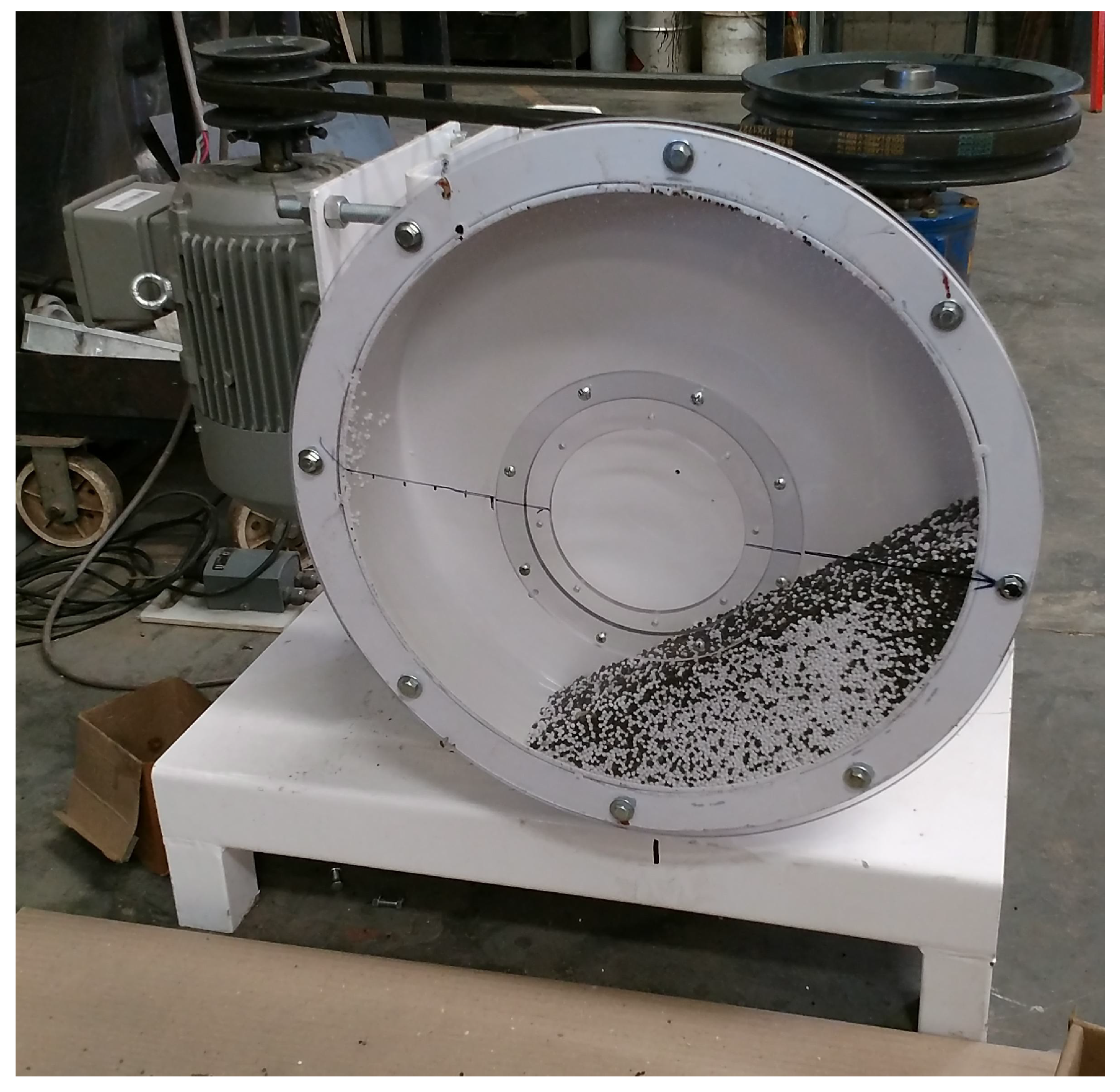
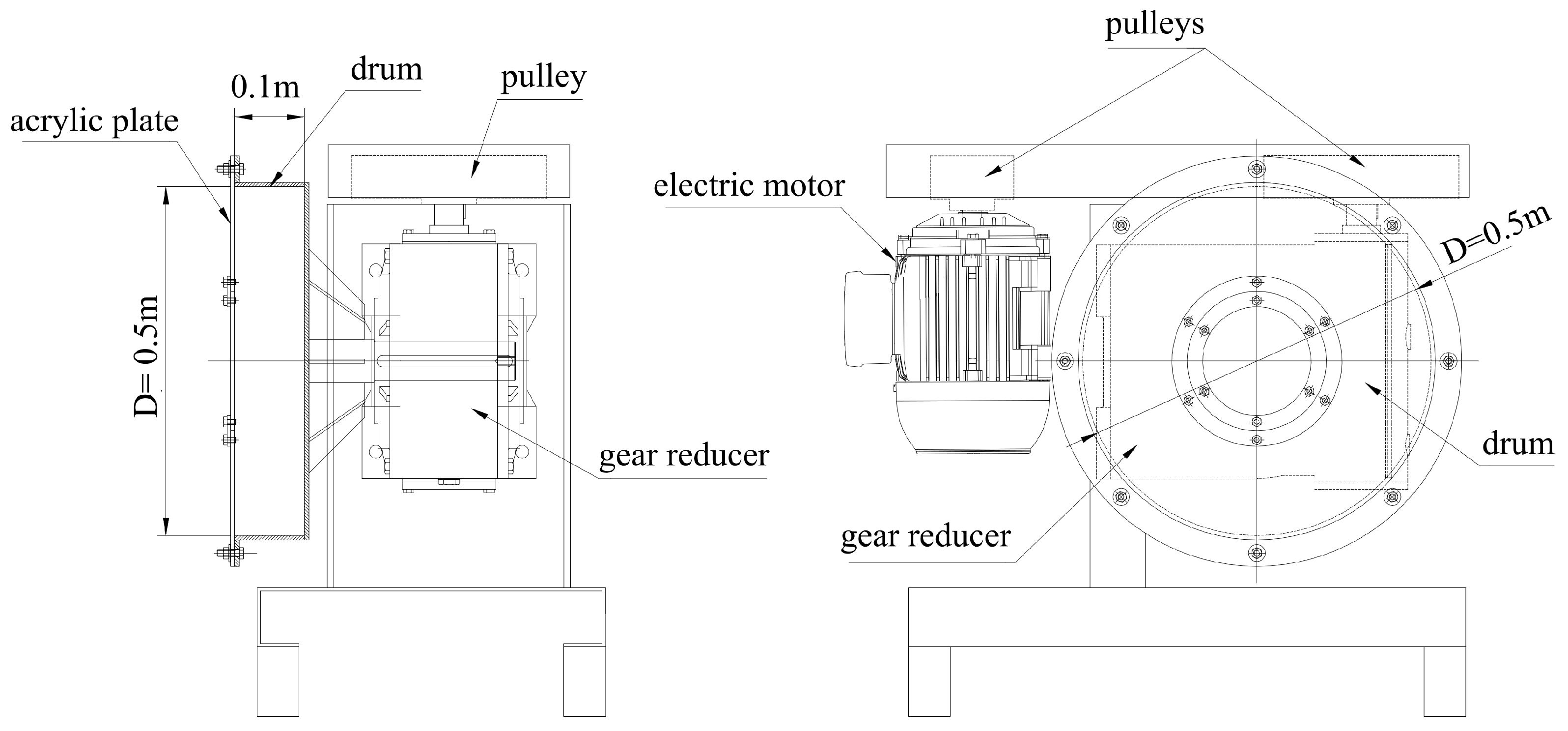
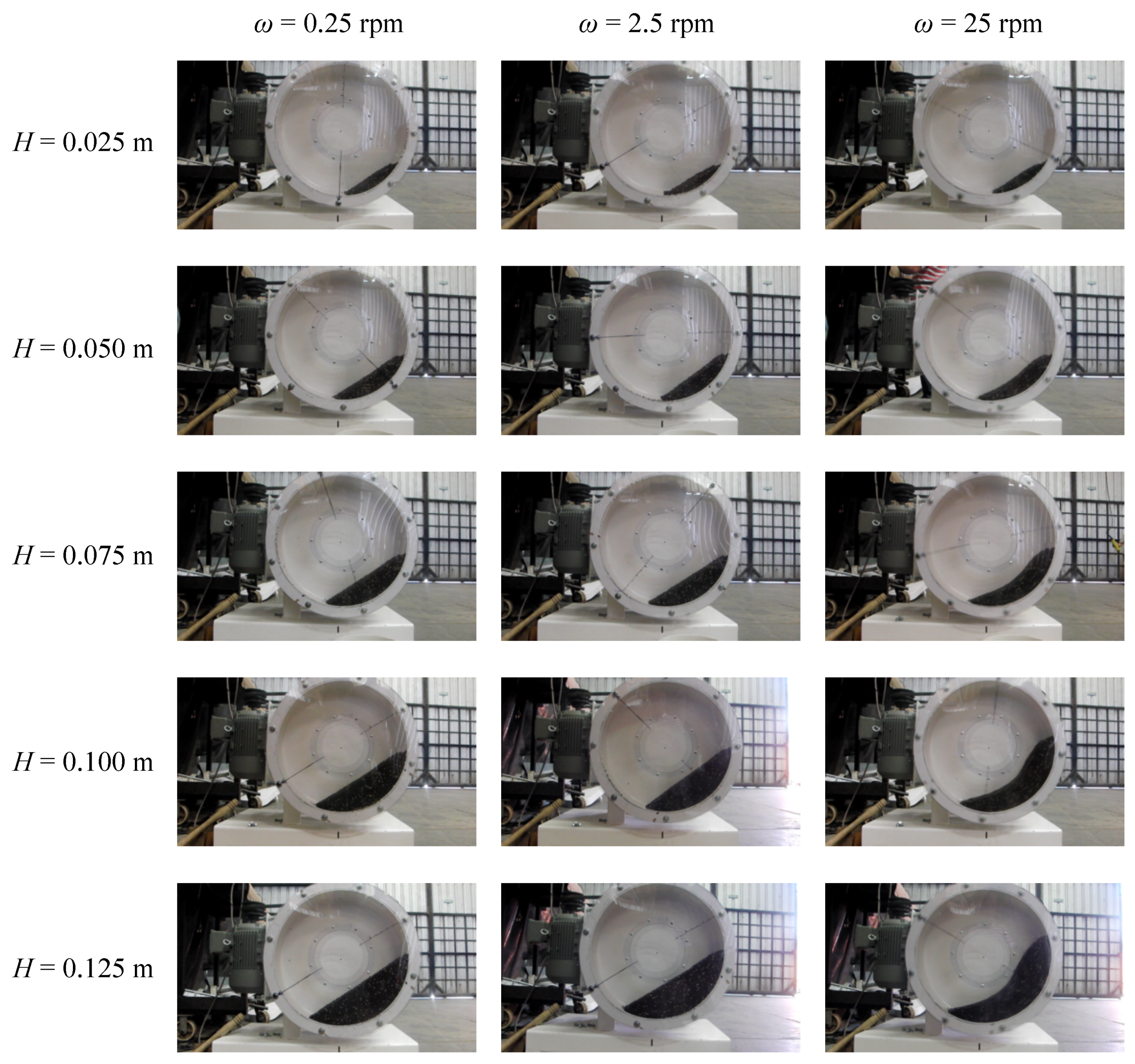
2. Experimental Setup

The laboratory drum consists of a 500-mm diameter and 100-mm width steel drum with its axis in a horizontal position (see Figure 1). The drum axis is coupled to a mechanical gear reducer that is driven by an electric motor via pulleys and belts. The speed of the motor can be modified using a frequency converter. All the parts and the general arrangement is shown in Figure 2.
The inner surface of the drum is painted with epoxy paint. The front cover of the drum is made of transparent plexiglass to visualize the movement of the granular material inside the drum. The cover has a circular hole in the middle through which the particles can be inserted or removed from the drum (as can be appreciated in the picture in Figure 1). The diameter of the hole is small enough such that the particles never leave the inner part of the drum during the experiments. After the drum is filled with particles, the surface of the bed is manually smoothed out and the height of the bed is measured at rest. The process of introducing or removing particles and the smoothing of the surface is repeated until the desired bed height is obtained.
The drum is filled with spherical particles of Di-Ammonium Phosphate (DAP) of 4 mm in diameter. A high-speed camera (Casio Exilim EX-FH20) with a resolution of 9.1 MP with up to 1000 fps is located in front of the bed to capture pictures and videos. Figure 3 shows pictures of the drum with different heights of filling and different rotational velocities.

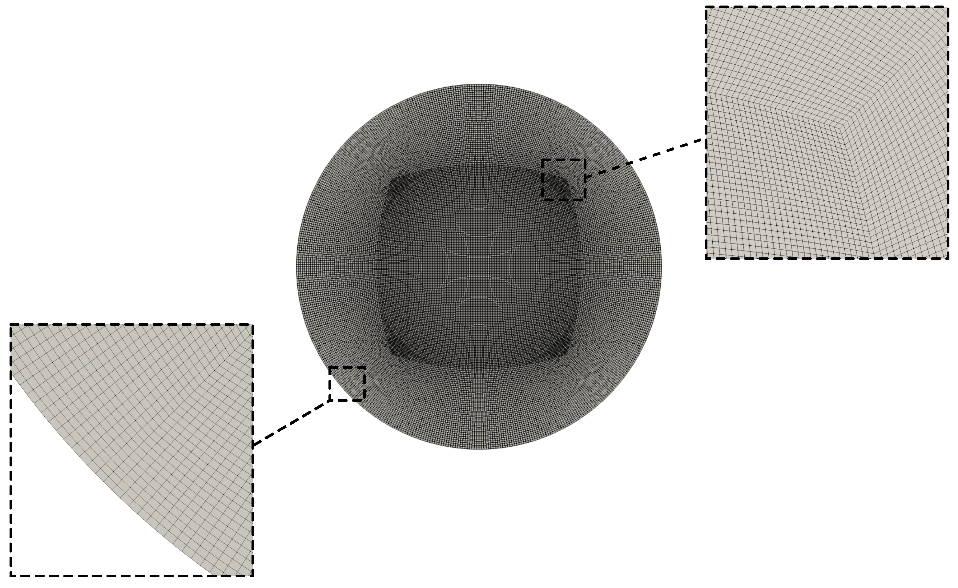
3. Computational Approach

3.1. Continuum Model (CM)

The continuum model (CM) is based on the Volume-Of-Fluid (VOF) method [46,47] implemented in the OpenFOAM(R) platform [48]. The model consists of the following equations of balance:
· u = 0
t ( ρ m u ) + · ( ρ m u u ) = · σ + ρ m g
α q t + · ( α q u ) + · [ α q ( 1 α q ) v q p ] = 0 .
Here, Equations (1)–(3) represent the continuity equation, the momentum balance, and the mass conservation of the continuous phase, respectively. u represents the center-of-volume velocity, ρ m is the density of the mixture, g is the gravity acceleration, α q is the solid volume fraction, and v q p is an ad-hoc relative velocity between phases suitable for free-surface compression [47]. The stress tensor may be written as:
σ = p I + η m γ ˙
γ ˙ = 1 2 ( u + u T )
where γ ˙ is the rate of deformation, p is the pressure field, and η m is the mixture viscosity defined as η m = α q η q + ( 1 α q ) η p , where η p is the dynamic viscosity of the air and η q is the viscosity of the granular media.
The current model considers the grains as a continuous media, therefore a rheology model must be defined for this phase. In this work, the μ ( I ) -rheology model is considered [41,42,50], where the viscosity is defined as:
η = μ ( I ) p | γ ˙ | .
Here, the μ ( I ) function is defined as:
μ ( I ) = μ 1 + ( μ 2 μ 1 ) ( I 0 / I + 1 )
I = | γ ˙ | d ( p / ρ q ) 0.5
where μ 1 , μ 2 , and I 0 are material parameters of the model, ρ q is the density of the solids, and d is the diameter of the particles.
This rheology was implemented on the general structure of the viscosity models of OpenFOAM(R) since it is not part of the standard distribution of the code. The velocity, pressure, and viscosity field are coupled by means of a segregated method of the SIMPLE-family [51,52]. In this model, a yield criterion should be reached as | γ | tends to zero. However, in these conditions, η would reach infinity and, following a general flow solver structure, this cannot be allowed to happen from a practical point of view. To fulfil the yield criteria, some authors propose to switch to a plastic model to correctly address the rigid body-like motion of the granular media [53,54]. In this work, the granular media is always treated as a fluid by considering that Equation (6) stands as long as η is below a certain threshold value. Whenever this threshold is reached, the viscosity is considered constant. This value can be defined by the user and it is usually high compared to any real fluid in order to mimic the rigid-body-like motion of the granular media. Although this combination of the multiphase flow model (VOF) and rheology model ( μ ( I ) rheology) is one of the many alternatives that can be adopted under a continuum approach, for simplicity, this approach will be referred to as the Continuum Model (CM) in the rest of the work.

3.2. Discrete Elements Method (DEM)

DEM is a Lagrangian method for modeling individual trajectories of every particle in a granular system. The equations of motion for a particle i with mass m i and moment of inertia I i are given by:
m i d v i d t = j F i j + F i g I i d ω i d t = j M i j
where v i and ω i are the translational and rotational velocities of particle i, F i j , and M i j are the contact force and torque acting on particle i by particle j, or by walls, F i g is the gravitational force. The summation is performed on all particles that are in contact with the particle i. The contact force F i j is comprised of normal and tangential contact forces denoted by F i j n and F i j t , respectively:
F i j = F i j n + F i j t
with
F i j n = ( k n δ n γ n v r n ) n i j F i j t = min { ( k t δ t + γ t v r t ) , μ | F i j n | } t i j
k n and k t are the normal and tangential spring coefficients, δ n and δ t are the relative normal and tangential displacements (overlaps), γ n and γ t are the normal and tangential damping coefficients, v r n and v r t are the normal and tangential components of the relative velocity between particles i and j, μ is the sliding friction coefficient, and n i j and t i j are the unit normal and tangential vectors.
The expressions for k n , k t , γ n , and γ t depend on the applied contact model. Here a non-linear damped Hertzian spring-dashpot model is used [55,56,57] and the coefficients are calculated from the material properties as follows:
k n = 4 3 E eq R eq δ n E eq = 1 ν i 2 E i + 1 ν j 2 E j 1 γ n = β 5 m eq k n G eq = 1 ν i G i + 1 ν j G j 1 k t = 8 G eq R eq δ n R eq = 1 R i + 1 R j 1 γ t = β 10 3 m eq k t m eq = 1 m i + 1 m j 1 β = ln e ( ln e ) 2 + π 2
where E is the Young’s modulus, ν is the Poisson ratio, G is the shear modulus, e is the coefficient of restitution, R is the particle radius, and m is the particle mass. For the contact of two particles i and j of different materials (urea and DAP), the equivalent properties (denoted by the subscript eq ) are used. Whereas for a collision of a particle i with a wall j the same relations are applied with R eq = R i and m eq = m i .
The torque acting on contacting particles is comprised of two terms. The rotational torque by contacts in the tangential direction M i j t , and the rolling resistant torque M i j r which is modeled here as a spring torque [58,59,60]:
M i j = M i j t + M i j r
with
M i j t = R n i j × F i j t M i j r = min { k r θ r , μ r R | F i j n | } ω ^ i j
where k r is the rolling stiffness which is assumed k r = k t R 2 [60]. In addition, θ r is relative rotation between two particles, μ r is the rolling friction coefficient, and ω ^ i j is the unit vector of the component of the relative angular velocity of particles.
Among all these parameters, the coefficient of restitution e, the coefficients of friction μ and μ r , and the mass m and radius R of the particles are regarded as given empirically and can be obtained from measurements or by calibrating simulations with experiments.

3.3. Test Cases

The assessment of the computational approaches and their experimental validations are based on four different test cases that seek to represent a wide range of regimes. For each case, a 3D cylindrical domain is considered using the geometry described in Section 2. Table 1 shows the bed depth, rotational velocity, and the regime observed experimentally, and Figure 4 shows the four regimes studied on a Bed Behavior Diagram (BBD).
For both computational methods, uniformly distributed spherical particles that have a 4-mm diameter are considered. The particles density for DAP is 1600 Kg/m 3 and the static friction coefficient is μ 1 = 0.53 . Case B and D require around 3 s to reach a steady state while Case C needed less than 10 seconds. The regime observed experimentally for Case A is slumpling, so a steady state is never reached, but a statistically steady state (where particles bed move back and forth at a fixed time period) is reached after the first 5 s from the beginning of the experiment.
Table 2 shows the numerical and physical parameters adopted for the CM.
For the CM simulations, an O-grid FVM mesh of 168.000 cells, with 5 cells in the depth, is adopted (as shown in Figure 5). Finer and coarser grids where tested beforehand and the current refinement was selected based on preserving a well-balanced relation between the computational cost involved in the simulations and the accuracy of the solution. It was observed that the solution fields do not change significantly for finer grids. A rotating wall boundary condition is imposed for all the surrounding walls of the drum. No turbulence model is used for the CM simulations and the air is treated as an incompressible fluid with properties at room thermal conditions.
DEM simulations were performed using LIGGGHTS which is an open-source software for modeling granular materials [49]. The stability of DEM simulations can be ensured by setting the time step equal to 20% of the Raleigh time step sizes (see LIGGGHTS documentation and also [61]).
Spherical particles (urea and DAP) with the same radii (2 mm) were used in all DEM simulations. Most of the constants were chosen on a purely empirical basis or were obtained by the calibration procedure (see below) and are summarized in Table 3.
The calibration procedure was the following. To determine the values of the coefficients of friction (sliding and rolling friction) for one type of material (DAP), two experiments were chosen: Static and dynamic angles of repose. The angle of repose is defined as the angle of inclination of the free surface to the horizontal of a conical bulk solid stack. It strongly depends on material properties such as sliding and rolling friction, but is not sensitive to the density of particles, Poisson’s ratio, or Young’s modulus [62,63,64]. Pile formation experiments in hoppers were performed to measure the static angle of repose, and the dynamic angle of repose was measured in the rotating drum tests. For the mixture of DAP and urea, the same parameter values were used except for the density and number of particles.
Particles were generated in a parallelepipedic region of the domain ( 400 × 47 × 100 mm) located 200 mm from the bottom of the drum. A uniform distribution in size but random in position was followed, with a rate of 200,000 particles/s, by generating new particles every 5000 timesteps. This is so because particles must leave the domain before new ones can be generated. As they are generated, particles fall by gravity and settle to the bottom of the drum by forming a pile. An insert region was used by filling almost the entire width of the drum (or length of the arch segment) to obtain a bed that covers all the necessary space without the need for too high a stack.
For the case of only one type of particle (DAP) a procedure of insertion and “smoothing” was performed. Once all particles were inserted (in a greater number than necessary to exceed the height of the bed) and they were at rest, particles located above a reference plane of the domain were eliminated to simulate a planar surface. In this initial condition, the volumes corresponding to two circular segments of 100 mm (thickness) and 75 mm and 125 mm (height) were occupied by 32,900 and 68,800 particles, respectively.
For the mixture of particles, the insertion was performed in two stages, one for each type of particle. Once all the particles of the lower layer were inserted and they were at rest, particles located above a reference plane of the domain were eliminated to simulate the planar interface between the two types of particles. Then, the second insertion stage was performed by generating the second layer with a height greater than the height of the bed. Once all particles were inserted and were at rest, a new reference plane removed the particles above this plane to simulate the flat surface layer. For the simulation of the mixture, particles were inserted forming two layers: One of urea with a high of 75 mm (31,200 particles of density 1300 kg/m 3 ) and the other of DAP at 50 mm high (34,900 particles of density 1600 kg/m 3 ).
It is important to note that the particle smoothing process was performed to achieve the same initial condition as the real experiment and was performed for all simulations. In the real experiments, the drum starts from rest with the particle layers in a horizontal position and the steady state speed of 25 rpm is reached after 1 complete revolution. In order to simulate this procedure, constant and staggered speeds were used for each 1 / 8 of a drum revolution in the first revolution. Then two additional revolutions were simulated at 25 rpm.

4. Results

The computational and experimental results are analyzed in three different aspects: The particles distribution inside the drum, the velocity of the particles, and the mixing patterns between two types of particles. In this section, these aspects are considered to evaluate the performance of both computational methods in terms of the accuracy of the solution and computational cost for the previously proposed cases. For each case, the solutions are analyzed in a qualitative (for the particles distribution and mixing patterns) and a quantitative manner (for the velocity field distribution) by comparing the results against the experimental observations. Each of the results shown below are taken after a steady state is reached (if they ever reach one), except for the mixing study where the transient evolution is analyzed.

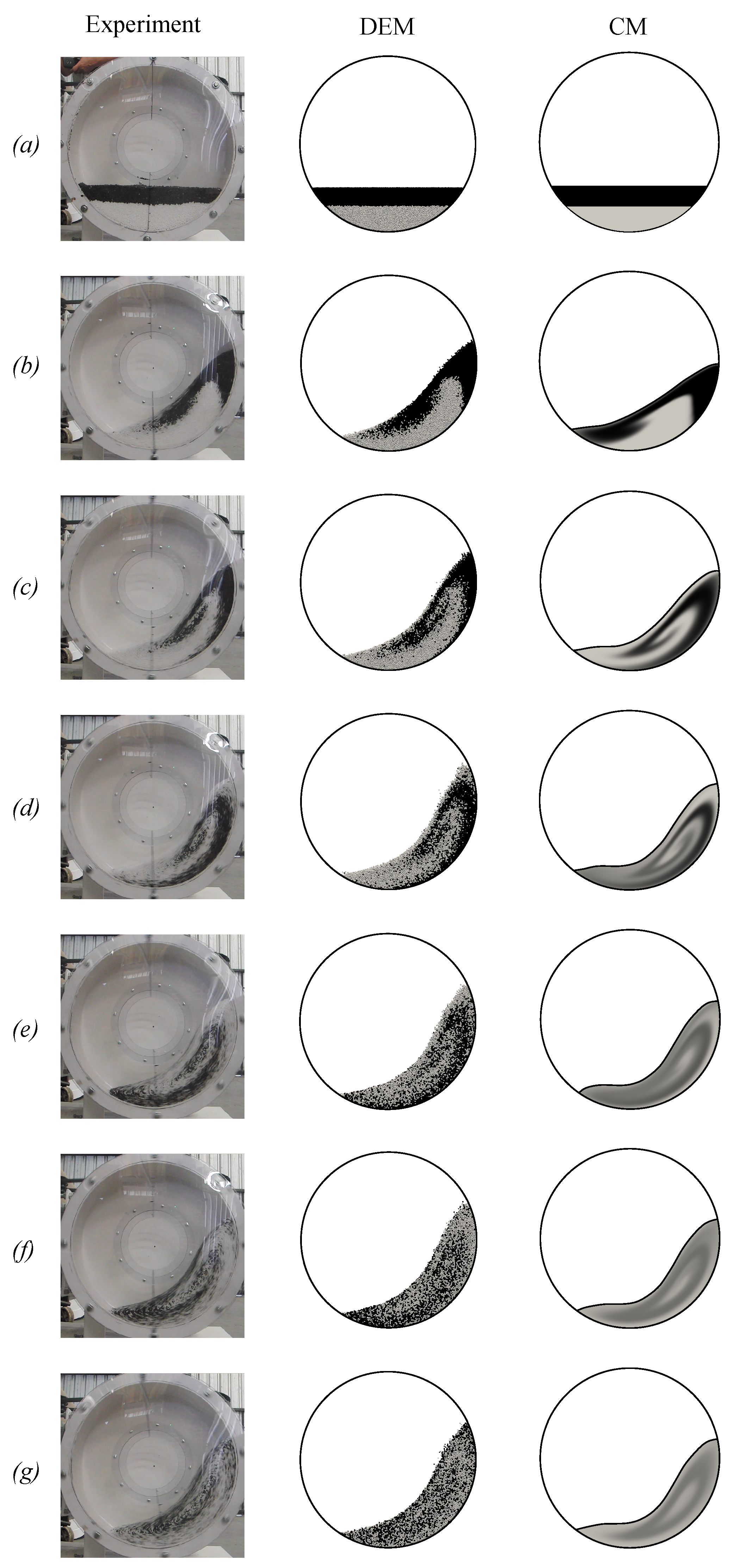
4.1. Particles Distribution

Figure 6 shows side-by-side the distribution of particles for the four proposed cases in the experiments and by computational simulations.
In particular, for Case A, DEM is able to predict the slumping regime as in the experiment, where the free surface of the bed of particles oscillates between two different angles and does not reach a steady position in time. Conversely, the continuum model does not capture this transient effect, showing a steady distribution with the plane of the free surface at an angle within the limits observed experimentally. This can be attributed to the absence of a yield criterion in the model above in which the pack of grains behave as a rigid body. Without this physical characteristic, the stick-and-slide effect of the slumping regime cannot occur.
For Case B, DEM predicts more splashing of particles in the right upper part of the bed compared to the experiment, while the continuum model does not. The same behavior is observed in Case C, where isolated particles move following the cylindrical wall of the drum and leave the dense core of particles before falling for their own weight.
At the left-most part of the particles bed, in each of the CM simulations, an unphysical “noise” in the solids fraction field might also be observed. This is due to the fact that particles are modeled as a continuum and the use of a refined grid with cells smaller than the particles size. In these conditions, it is possible to obtain intermediate volume fractions (between 0 and 1) at certain places where there should be only particles or air. In any case, the amount of solids fraction here represents less than 0.1% of the granular bed which does not affect the general results.
Although in general the results of the CM are in good agreement with the experiments, the regimes with higher velocities (Case B and D) exhibit a lack of accuracy to predict the length of the “tail” of the bed surface (bottom-left part region of the bed). This could be observed in more detail in Figure 7, where the interfaces between the bed of particles and air are plotted simultaneously for the three methods of observation/prediction. The reason behind the differences is that the CM is preserving the initial volume while the volume of mixture in DEM and experiment expands. This is due to the presence of air that percolates through the core of the bed as the drum is rotating. This effect is emphasized at higher velocities (Case B and D) and cannot be captured by the CM. For the continuum model, the bed surface is defined as an isosurface with 0.5 of concentration.
Overall, the distribution of particles is accurately predicted by the CM and DEM, with the exception of Case A where the slumping effect cannot be captured by CM. In addition, for Case D, the bed surface predicted by CM does not match perfectly with the results of the experiment and DEM.
Regarding the computational costs, the simulations of Case C are taken as a reference. To achieve a steady distribution of particles for this problem, 12 s of physical time is required. Both methods of simulation use a set of numerical parameters that optimize the costs for a similar level of accuracy of the solution. This is achieved in practice by repeating the simulations, each time modifying certain numerical parameters with the purpose of increasing the time step as long as the numerical stability is not lost. For DEM, the simulation required 10.530 s, where a maximum time step of Δ t = 2 × 10 5 s was used. For CM, the simulation required 8.340 s, where a fixed time step of Δ t = 2 × 10 3 s was needed. For these conditions, and given the FVM mesh adopted, CM saves around 20% of computational costs compared to DEM. While this saving could be considered marginal given the accuracy requirements for this problem and the overall time consumed (no more than a few hours on a personal computer), the scale of the problem should be taken into account in this analysis. This problem considers a lab-scale configuration with particles of a few millimetres of diameter, where the use of DEM can still be recommended. However, when an industrial-scale problem is considered, the use of DEM becomes a subject of debate and clustering of particles should be considered for the simulation, otherwise the computational costs could make the simulation prohibitive. In these conditions, the use of a CM approach becomes a promising alternative since the computational cost involved does not scale with the dimension of the problem necessarily. Moreover, the relative size of the particles compared to the size of the domain is almost irrelevant to the overall time consumption, unlike in DEM.

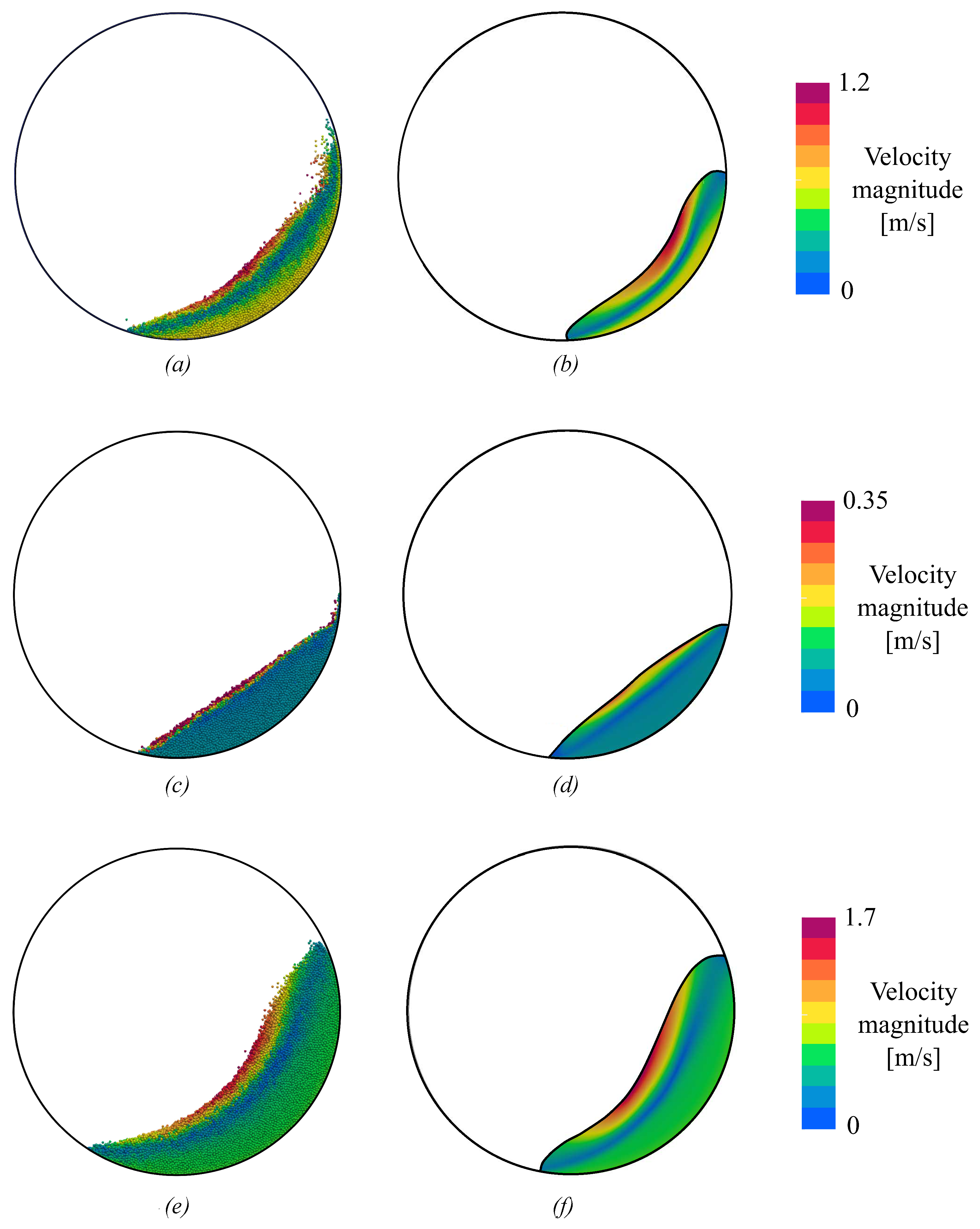
4.2. Velocity Distribution

The velocity of the particles inside the drum is a key aspect to compare between simulations and the experiment. For Case A, Figure 8a shows the magnitude of the velocity predicted with DEM during the sticking period of the slumping regime, where the particles move with the walls at the corresponding velocity as it were a rigid body (i.e., v = ω r ). Figure 8b shows the distribution of the tangential component of the velocity with DEM and experimentally. For these conditions, the DEM exhibits a very high level of agreement in both the instantaneous velocity field and the period of stick and slide observed in the experiment. The CM results are omitted for this case since the general regime cannot be captured.
Figure 9 shows the simulation predictions of the velocity field magnitude for a transitional regime (Case B), a rolling regime (Case C), and a cascading regime (Case D), respectively.
In the rolling regime, both approaches show a quasi-planar bed surface where the particles are moving downward at a high velocity near the interface. This layer of high velocity is very thin and the particles rapidly change direction as we move far from the centre of the drum until reaching the rotating wall velocity. In the transitional and cascading regimes, the maximum velocity is reached close to the part of the bed surface that is farthest from the drum cylindrical wall, where the particles move downward in the opposite direction of the rotating wall. Unlike the rolling regime, here the high-velocity layer is broader until it reaches zero tangential velocity. Once again, both models show similar trends.
Figure 10 shows the tangential velocity profile on a radial direction at 35º from the vertical direction for rolling and cascading regimes. The simulation results are plotted along with the velocity measured experimentally at certain positions. The experimental results are computed based on the relative position of tracer particles inside the bed analyzing each frame of a high-quality video filmed at 25 fps. The error bars amplitude are computed based on the uncertainty of the position measurement of the tracer particles divided by the time span between frames.
In general, the granular phase velocity is null until the bed surface is reached and then it rapidly becomes maximum and decreases until it changes direction as we move far from the centre. Both computational models are in agreement with the experiment and with each other in the region close to the rotating wall and present more differences close to the bed surface. However, the general trend is in agreement and there is no one technique that stands out from the other in terms of accuracy of the solution in comparison to the experiment. In fact, for the rolling regime, the experiment seems to be close in agreement with the DEM results in the backward flowing region, but it is the opposite for the cascading regime, where the continuum model seems to be closer to the experimental observation. It is worth mentioning that DEM seems to slightly overestimate the tangential velocity in comparison to the continuum approach in the backward flowing region.

4.3. Mixing Patterns

This section focuses on the capability of both approaches to accurately measure the mixing of two materials inside the drum rotating at a cascading regime. Figure 11 shows the distribution of particles inside the drum while being accelerated from 0 to 25 rpm. The drum is filled with particles with two colors (black and white) initially segregated and each frame represents half of a cycle (three cycles in total).
For the DEM simulation, particles were inserted forming two layers: One of urea at 75 mm high (31,200 particles) and the other of DAP at 50 mm high (34,900 particles). In the real experiment, the drum starts from rest with the particle layers in a horizontal position and the steady-state speed of 25 rpm is reached after two cycles.
Both computational approaches are tested and compared against the experimental observations. In general, both approaches are apt to predict the amount of time needed to mix the two materials from qualitative observation of the results.
At a closer analysis, the DEM approach is in very close agreement with the qualitative patterns observed experimentally. On the other hand, the continuum model is slower to reach the maximum height of the bed but eventually does once the steady regime is established. This drawback of the CM model may be attributed to the absence of non-local effects on the model. Henann et al. [65] have shown that the correct shear layer that takes place in cylindrical geometries cannot be captured with the standard μ ( I ) -rheology and non-local effects must be included in the model to accurately predict the size of the shear bands. This type of problem is not far from a rotating drum arrangement where, if the gravity is not considered, the rate at which the shear bands are formed could be different between the experiment and a local rheology model. Eventually, due to the presence of gravity, the non-locality aspects of the rheological model becomes non-relevant for predicting the steady-state flow and particles distribution but might explain the inaccuracies in the transient evolution.

5. Conclusions

In this work, the performance of discrete and continuum approaches for modeling the solids motion inside a rotating drum at different regimes has been studied. To achieve this, a pilot-plant rotating drum experiment filled with DAP spherical particles with a 4-mm diameter, was mounted with a plexiglass cover to observe the flow patterns using a high-speed camera. The DEM simulations were performed with the open-source code LIGGGHTS(R), while a VOF solver of the OpenFOAM(R) platform was adopted for the continuum approach. To account for the granular flow dynamics in this context, an implementation of the μ ( I ) -rheology was made on the general structure of the viscosity models library of the code.
For evaluating the performance of the computational approaches, four different test cases at different regimes were considered. The accuracy of the results was analyzed in terms of solids distribution, particles velocities, and mixing patterns. The main findings may be summarized as follows:
  • The solids distribution for each regime was correctly predicted with both techniques, except for the slumping regime, which could not be captured by the CM approach. This was attributed to the use of a high-viscosity threshold instead of a yield criterion in the implementation of the rheology model. In the fastest regimes, DEM predicted more splashing of particles than the experimental observations;
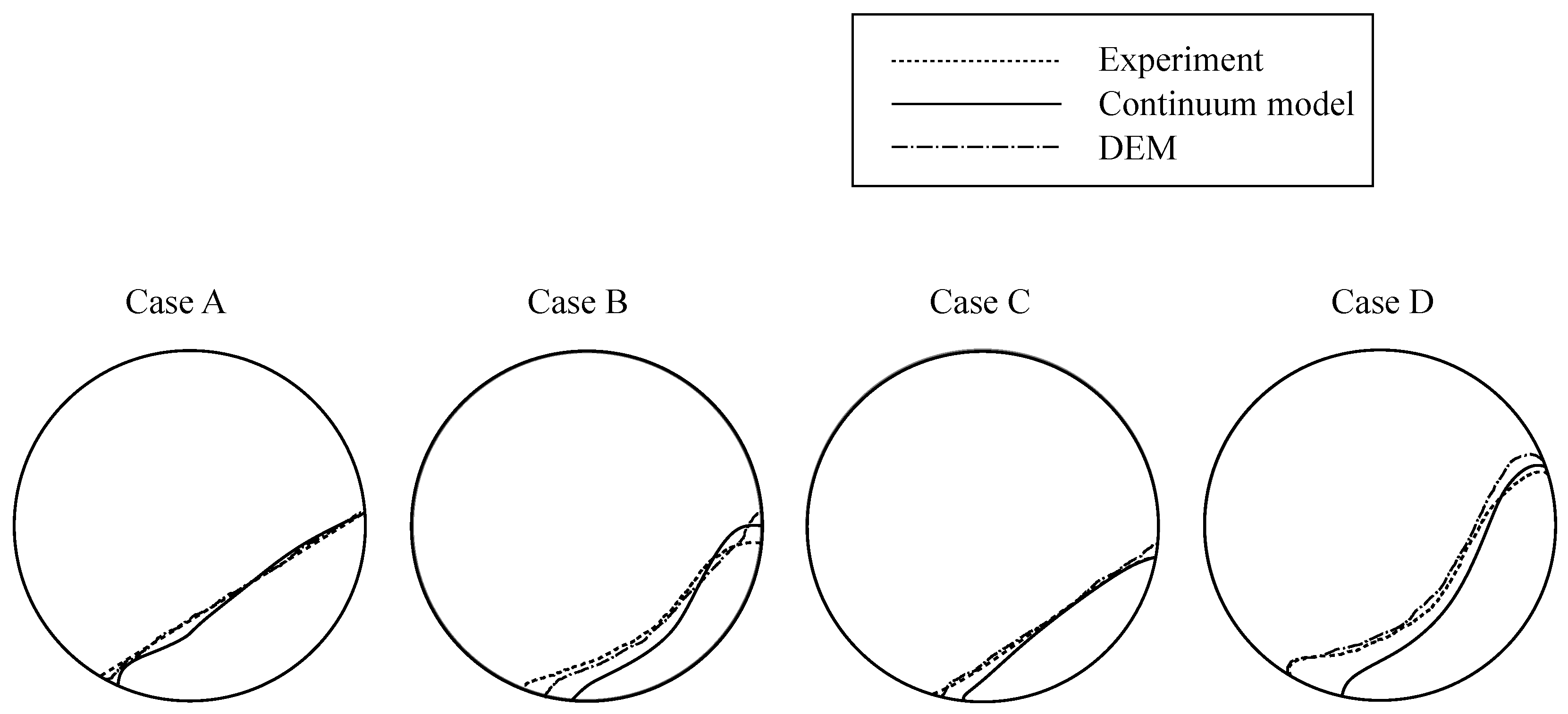
  • The velocity of the particles predicted by the models was mostly in agreement with the experimental results. Neither of the computational models stood out over the other in this regard as both tend to detach more from the experimental observations where the material flow backwards relative to the rotation of the drum;
  • The rate of mixing of two different materials in a cascading regime was well predicted by both models, reaching a fairly similar level of mixing at different instants in time. While the DEM results were in very good agreement with the experiments, the CM predicted a slower dragging of the material as the system was accelerated but reaching similar steady-state profiles of the interface between the bed of particles and the air. This drawback might be attributed to the lack of non-local effects and a yield criterion that reign over the inertial regime at slow speeds;
  • In the rolling regime, CM saved around 20% of computational time compared to DEM, both with an optimized set of numerical parameters. This suggests that, when the dimensions of the problem shifted from pilot-plant to industrial-scale, CM might still be suitable while the computational costs of DEM might become prohibitive.
In general, both techniques were able to predict the granular flow patterns in most of the regimes analyzed. The CM model used in this work needs to incorporate more phenomenological features to predict with the same level of accuracy as DEM for lab and pilot-plant scales. This indicates that a more comprehensive rheological model is needed but it is yet to be proven if an Euler-Euler approach (such as the Two-Fluids Model) instead of VOF could yield more accurate predictions. The results of this study suggest that a continuum model based on the μ ( I ) -rheology (with a pressure-dependent viscosity and a yield criterion) enhanced with non-local effects, in contrast to DEM, would be an interesting approach for simulating industrial-scale rotating drums, by meeting both accuracy and computational cost requirements.

Author Contributions

Conceptualization: C.M.V., S.M.D. and N.M.N.; Methodology: C.M.V., S.M.D., S.E.B., G.D.P. and N.M.N.; Supervision: N.M.N., S.E.B. and J.M.R. provided the experimental facilities. All the authors contributed to the discussion, the writing, and the revision of the paper. All authors read and agreed to the published version of the manuscript.

Funding

This research was funded by ANPCyT grant PICT 2016-2908, ASACTEI grant 1010-009-16, ASACTEI grant AC-00010-18, Universidad Tecnológica Nacional through Research Program ASUTNRA0007817 and CONICET for the funding through doctoral and postdoctoral scholarships.

Institutional Review Board Statement

Not applicable.

Informed Consent Statement

Not applicable.

Data Availability Statement

Data are contained within the present article.

Acknowledgments

The authors acknowledge the Universidad Nacional de Rosario, Universidad Nacional del Litoral, and Universidad Tecnológica Nacional (Facultad Regional Santa Fe and Facultad Regional Rafaela) for their support. The authors also wish to thank Sebastian Jappert from DEISA S.A. for his collaboration with the experimental setup.

Conflicts of Interest

The authors declare no conflict of interest.

References

  1. Henein, H.; Brimacombe, J.; Watkinson, A. Experimental study of transverse bed motion in rotary kilns. Metall. Trans. B 1983, 14, 191–205. [Google Scholar] [CrossRef]
  2. Henein, H.; Brimacombe, J.; Watkinson, A. The modeling of transverse solids motion in rotary kilns. Metall. Trans. B 1983, 14, 207–220. [Google Scholar] [CrossRef]
  3. Mellmann, J. The transverse motion of solids in rotating cylinders—Forms of motion and transition behavior. Powder Technol. 2001, 118, 251–270. [Google Scholar] [CrossRef]
  4. Ding, Y.; Forster, R.; Seville, J.; Parker, D. Segregation of granular flow in the transverse plane of a rolling mode rotating drum. Int. J. Multiph. Flow 2002, 28, 635–663. [Google Scholar] [CrossRef]
  5. Aissa, A.A.; Duchesne, C.; Rodrigue, D. Effect of friction coefficient and density on mixing particles in the rolling regime. Powder Technol. 2011, 212, 340–347. [Google Scholar] [CrossRef]
  6. Liu, X.Y.; Specht, E.; Mellmann, J. Experimental study of the lower and upper angles of repose of granular materials in rotating drums. Powder Technol. 2005, 154, 125–131. [Google Scholar] [CrossRef]
  7. Chou, S.; Hsiau, S. Dynamic properties of immersed granular matter in different flow regimes in a rotating drum. Powder Technol. 2012, 226, 99–106. [Google Scholar] [CrossRef]
  8. Huang, A.; Kuo, H. A study on the transition between neighbouring drum segregated bands and its application to functionally graded material production. Powder Technol. 2011, 212, 348–353. [Google Scholar] [CrossRef]
  9. Orpe, A.V.; Khakhar, D. Scaling relations for granular flow in quasi-two-dimensional rotating cylinders. Phys. Rev. E 2001, 64, 031302. [Google Scholar] [CrossRef]
  10. Santos, D.A.; Barrozo, M.A.; Duarte, C.R.; Weigler, F.; Mellmann, J. Investigation of particle dynamics in a rotary drum by means of experiments and numerical simulations using DEM. Adv. Powder Technol. 2016, 27, 692–703. [Google Scholar] [CrossRef]
  11. Santos, D.A.; Dadalto, F.O.; Scatena, R.; Duarte, C.R.; Barrozo, M.A. A hydrodynamic analysis of a rotating drum operating in the rolling regime. Chem. Eng. Res. Des. 2015, 94, 204–212. [Google Scholar] [CrossRef]
  12. Marigo, M.; Cairns, D.; Davies, M.; Ingram, A.; Stitt, E. A numerical comparison of mixing efficiencies of solids in a cylindrical vessel subject to a range of motions. Powder Technol. 2012, 217, 540–547. [Google Scholar] [CrossRef]
  13. Xu, Y.; Xu, C.; Zhou, Z.; Du, J.; Hu, D. 2D DEM simulation of particle mixing in rotating drum: A parametric study. Particuology 2010, 8, 141–149. [Google Scholar] [CrossRef]
  14. Liu, P.; Yang, R.; Yu, A. DEM study of the transverse mixing of wet particles in rotating drums. Chem. Eng. Sci. 2013, 86, 99–107. [Google Scholar] [CrossRef]
  15. Watanabe, H. Critical rotation speed for ball-milling. Powder Technol. 1999, 104, 95–99. [Google Scholar] [CrossRef]
  16. Chand, R.; Khaskheli, M.A.; Qadir, A.; Ge, B.; Shi, Q. Discrete particle simulation of radial segregation in horizontally rotating drum: Effects of drum-length and non-rotating end-plates. Phys. A Stat. Mech. Its Appl. 2012, 391, 4590–4596. [Google Scholar] [CrossRef]
  17. Zhang, L.; Jiang, Z.; Mellmann, J.; Weigler, F.; Herz, F.; Bück, A.; Tsotsas, E. Influence of the number of flights on the dilute phase ratio in flighted rotating drums by PTV measurements and DEM simulations. Particuology 2021, 56, 171–182. [Google Scholar] [CrossRef]
  18. Huang, A.; Cheng, T.; Hsu, W.; Huang, C.; Kuo, H. DEM study of particle segregation in a rotating drum with internal diameter variations. Powder Technol. 2021, 378, 430–440. [Google Scholar] [CrossRef]
  19. Harish, V.; Cho, M.; Shim, J. Effect of rotating cylinder on mixing performance in a cylindrical double-ribbon mixer. Appl. Sci. 2019, 9, 5179. [Google Scholar] [CrossRef] [Green Version]
  20. Yang, R.; Yu, A.; McElroy, L.; Bao, J. Numerical simulation of particle dynamics in different flow regimes in a rotating drum. Powder Technol. 2008, 188, 170–177. [Google Scholar] [CrossRef]
  21. Gan, J.; Zhou, Z.; Yu, A. A GPU-based DEM approach for modeling of particulate systems. Powder Technol. 2016, 301, 1172–1182. [Google Scholar] [CrossRef]
  22. Lun, C.; Savage, S.B.; Jeffrey, D.; Chepurniy, N. Kinetic theories for granular flow: Inelastic particles in Couette flow and slightly inelastic particles in a general flowfield. J. Fluid Mech. 1984, 140, 223–256. [Google Scholar] [CrossRef]
  23. Venier, C.M.; Damian, S.M.; Nigro, N.M. Numerical aspects of Eulerian gas–particles flow formulations. Comput. Fluids 2016, 133, 151–169. [Google Scholar] [CrossRef]
  24. Venier, C.M.; Marquez Damian, S.; Nigro, N.M. Assessment of gas-particle flow models for pseudo-2D fluidized bed applications. Chem. Eng. Commun. 2018, 205, 456–478. [Google Scholar] [CrossRef]
  25. Venier, C.M. Resolución Computacional de Flujos Multifásicos Granulares Por Métodos Eulerianos. Ph.D. Thesis, Universidad Nacional del Litoral, Santa Fe, Argentina, 2018. [Google Scholar]
  26. Gidaspow, D. Multiphase Flow and Fluidization: Continuum and Kinetic Theory Descriptions; Academic Press: Cambridge, MA, USA, 1994. [Google Scholar]
  27. Enwald, H.; Peirano, E.; Almstedt, A.E. Eulerian two-phase flow theory applied to fluidization. Int. J. Multiph. Flow 1996, 22, 21–66. [Google Scholar] [CrossRef]
  28. Taghipour, F.; Ellis, N.; Wong, C. Experimental and computational study of gas–solid fluidized bed hydrodynamics. Chem. Eng. Sci. 2005, 60, 6857–6867. [Google Scholar] [CrossRef]
  29. Loha, C.; Chattopadhyay, H.; Chatterjee, P.K. Assessment of drag models in simulating bubbling fluidized bed hydrodynamics. Chem. Eng. Sci. 2012, 75, 400–407. [Google Scholar] [CrossRef]
  30. Makkawi, Y.T.; Wright, P.C.; Ocone, R. The effect of friction and inter-particle cohesive forces on the hydrodynamics of gas–solid flow: A comparative analysis of theoretical predictions and experiments. Powder Technol. 2006, 163, 69–79. [Google Scholar] [CrossRef]
  31. Passalacqua, A.; Fox, R.O. Implementation of an iterative solution procedure for multi-fluid gas–particle flow models on unstructured grids. Powder Technol. 2011, 213, 174–187. [Google Scholar] [CrossRef]
  32. Patil, D.; van Sint Annaland, M.; Kuipers, J. Critical comparison of hydrodynamic models for gas–solid fluidized beds—Part I: Bubbling gas–solid fluidized beds operated with a jet. Chem. Eng. Sci. 2005, 60, 57–72. [Google Scholar] [CrossRef]
  33. Patil, D.; van Sint Annaland, M.; Kuipers, J. Critical comparison of hydrodynamic models for gas–solid fluidized beds—Part II: Freely bubbling gas–solid fluidized beds. Chem. Eng. Sci. 2005, 60, 73–84. [Google Scholar] [CrossRef]
  34. Santos, D.; Duarte, C.; Barrozo, M. Segregation phenomenon in a rotary drum: Experimental study and CFD simulation. Powder Technol. 2016, 294, 1–10. [Google Scholar] [CrossRef]
  35. Rong, W.; Feng, Y.; Schwarz, P.; Witt, P.; Li, B.; Song, T.; Zhou, J. Numerical study of the solid flow behavior in a rotating drum based on a multiphase CFD model accounting for solid frictional viscosity and wall friction. Powder Technol. 2020, 361, 87–98. [Google Scholar] [CrossRef]
  36. Rong, W.; Li, B.; Feng, Y.; Schwarz, P.; Witt, P.; Qi, F. Numerical analysis of size-induced particle segregation in rotating drums based on Eulerian continuum approach. Powder Technol. 2020, 376, 80–92. [Google Scholar] [CrossRef]
  37. Machado, M.; Nascimento, S.; Duarte, C.; Barrozo, M. Boundary conditions effects on the particle dynamic flow in a rotary drum with a single flight. Powder Technol. 2017, 311, 341–349. [Google Scholar] [CrossRef]
  38. Yin, H.; Zhang, M.; Liu, H. Numerical simulation of three-dimensional unsteady granular flows in rotary kiln. Powder Technol. 2014, 253, 138–145. [Google Scholar] [CrossRef]
  39. Schaeffer, D.G. Instability in the evolution equations describing incompressible granular flow. J. Differ. Equ. 1987, 66, 19–50. [Google Scholar] [CrossRef] [Green Version]
  40. Johnson, P.C.; Jackson, R. Frictional–collisional constitutive relations for granular materials, with application to plane shearing. J. Fluid Mech 1987, 176, 67–93. [Google Scholar] [CrossRef]
  41. Jop, P.; Forterre, Y.; Pouliquen, O. A constitutive law for dense granular flows. Nature 2006, 441, 727–730. [Google Scholar] [CrossRef] [PubMed] [Green Version]
  42. Da Cruz, F.; Emam, S.; Prochnow, M.; Roux, J.N.; Chevoir, F. Rheophysics of dense granular materials: Discrete simulation of plane shear flows. Phys. Rev. E 2005, 72, 021309. [Google Scholar] [CrossRef] [Green Version]
  43. GDR MiDi. On dense granular flows. Eur. Phys. J. 2004, 14, 341–365. [Google Scholar]
  44. De Monaco, G.; Greco, F.; Maffettone, P. Flow of Dry Grains Inside Rotating Drums. In Challenges in Mechanics of Time-Dependent Materials, Volume 2; Springer: Berlin, Germany, 2015; pp. 121–129. [Google Scholar]
  45. Arseni, A.M.; De Monaco, G.; Greco, F.; Maffettone, P.L. Granular flow in rotating drums through simulations adopting a continuum constitutive equation. Phys. Fluids 2020, 32, 093305. [Google Scholar] [CrossRef]
  46. Hirt, C.W.; Nichols, B.D. Volume of fluid (VOF) method for the dynamics of free boundaries. J. Comput. Phys. 1981, 39, 201–225. [Google Scholar] [CrossRef]
  47. Márquez Damián, S.; Nigro, N.M. An extended mixture model for the simultaneous treatment of small-scale and large-scale interfaces. Int. J. Numer. Methods Fluids 2014, 75, 547–574. [Google Scholar] [CrossRef]
  48. Weller, H.G.; Tabor, G.; Jasak, H.; Fureby, C. A tensorial approach to computational continuum mechanics using object-oriented techniques. Comput. Phys. 1998, 12, 620–631. [Google Scholar] [CrossRef]
  49. Kloss, C.; Goniva, C.; Hager, A.; Amberger, S.; Pirker, S. Models, algorithms and validation for opensource DEM and CFD-DEM. Prog. Comput. Fluid Dyn. An Int. J. 2012, 12, 140–152. [Google Scholar] [CrossRef]
  50. Forterre, Y.; Pouliquen, O. Flows of dense granular media. Annu. Rev. Fluid Mech. 2008, 40, 1–24. [Google Scholar] [CrossRef] [Green Version]
  51. Patankar, S.V.; Spalding, D.B. A calculation procedure for heat, mass and momentum transfer in three-dimensional parabolic flows. Int. J. Heat Mass Transf. 1972, 15, 1787–1806. [Google Scholar] [CrossRef]
  52. Issa, R.I. Solution of the implicitly discretised fluid flow equations by operator-splitting. J. Comput. Phys. 1986, 62, 40–65. [Google Scholar] [CrossRef]
  53. Kamrin, K. Nonlinear elasto-plastic model for dense granular flow. Int. J. Plast. 2010, 26, 167–188. [Google Scholar] [CrossRef] [Green Version]
  54. Dunatunga, S.; Kamrin, K. Continuum modeling and simulation of granular flows through their many phases. J. Fluid Mech. 2015, 779, 483–513. [Google Scholar] [CrossRef] [Green Version]
  55. Tsuji, Y.; Tanaka, T.; Ishida, T. Lagrangian numerical simulation of plug flow of cohesionless particle in a horizontal pipe. Powder Technol. 1992, 71, 239–250. [Google Scholar] [CrossRef]
  56. Di Renzo, A.; Di Maio, F. Comparison of contact-force models for the simulation of collisions in DEM-based granular flow codes. Chem. Eng. Sci. 2004, 59, 525–541. [Google Scholar] [CrossRef]
  57. Di Renzo, A.; Di Maio, F. An improved integral non-linear model for the contact of particles in distinct element simulations. Chem. Eng. Sci. 2005, 60, 1303–1312. [Google Scholar] [CrossRef]
  58. Iwashita, K.; Oda, M. Rolling resistance at contacts in simulation of shear band development by DEM. J. Eng. Mech. 1998, 124, 285–292. [Google Scholar] [CrossRef]
  59. Iwashita, K.; Oda, M. Micro-Deformation Mechanism of Shear Banding Process Based on Modified Distinct Element Method. Powder Technol. 2000, 2, 192–205. [Google Scholar] [CrossRef]
  60. Ai, J.; Chen, J.F.; Rotter, J.; Ooi, J. Assessment of rolling resistance models in discrete element simulations. Powder Technol. 2011, 206, 269–282. [Google Scholar] [CrossRef]
  61. Jensen, A.; Fraser, K.; Laird, G. Improving the Precision of Discrete Element Simulations through Calibration Models. In Proceedings of the 13 th International LS-DYNA Users Conference, Dearborn, MI, USA, 8–10 June 2014; pp. 1–12. [Google Scholar]
  62. Zhou, Y.; Wright, B.; Yang, R.; Xu, B.; Yu, A. Rolling friction in the dynamic simulation of sandpile formation. Phys. A Stat. Mech. Its Appl. 1999, 269, 536–553. [Google Scholar] [CrossRef]
  63. Zhou, Y.; Xu, B.; Yu, A.; Zulli, P. An experimental and numerical study of the angle of repose of coarse spheres. Powder Technol. 2002, 125, 45–54. [Google Scholar] [CrossRef]
  64. Frankowski, P.; Morgeneyer, M. Calibration and validation of DEM rolling and sliding friction coefficients in angle of repose and shear measurements. AIP Conf. Proc. 2013, 1542, 851. [Google Scholar]
  65. Henann, D.L.; Kamrin, K. Continuum modeling of secondary rheology in dense granular materials. Phys. Rev. Lett. 2014, 113, 178001. [Google Scholar] [CrossRef] [PubMed] [Green Version]
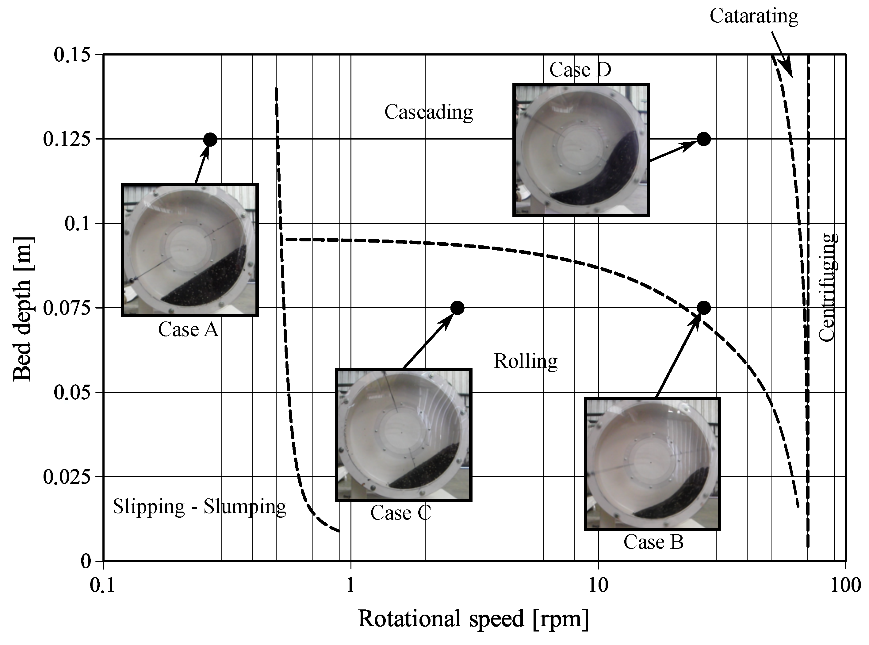
Figure 1. Experimental setup.
Applsci 11 10090 g001
Figure 2. Scheme of the device with all the parts and dimensions of the drum.
Applsci 11 10090 g002
Figure 3. Experimental solids distribution at different rotational velocities and initial bed heights.
Applsci 11 10090 g003
Figure 4. Bed Behavior Diagram for DAP.
Applsci 11 10090 g004
Figure 5. Grid adopted for the CM simulations.
Applsci 11 10090 g005
Figure 6. Particles distribution for the four test cases: (a) Experiment, (b) DEM, and (c) CM.
Applsci 11 10090 g006
Figure 7. Interface between air and the bed of particles for the proposed regimes comparing experiment and simulations.
Applsci 11 10090 g007
Figure 8. Velocity field for Case A: (a) Velocity field magnitude with DEM and (b) normalizedtangential component of the velocity as a function of a radial direction at 35º from a vertical line measured experimentally and through simulation.
Applsci 11 10090 g008
Figure 9. Velocity field magnitude for (a) Case B with DEM, (b) Case B with CM, (c) Case C with DEM, (d) Case C with CM, (e) Case D with DEM, and (f) Case D with CM.
Applsci 11 10090 g009
Figure 10. Tangential velocity as a function of a radial direction at 35° from a vertical line measured experimentally and through simulation for (a) Case B, (b), Case C, and (c) Case D.
Applsci 11 10090 g010
Figure 11. Particles distribution over time for two materials initially segregated and accelerated until reaching a steady regime. (a) At rest, (b) after 0.5 cycle, (c) 1 cycle, (d) 1.5 cycles, (e) 2 cycles, (f) 2.5 cycles, and (g) 3 cycles.
Applsci 11 10090 g011
Table 1. Test cases.
CaseBed Depth [m]Rotational Speed [rpm]Observed Regime
A 0.125 0.25 Slumping
B 0.075 25Transitional (Rolling/Cascading)
C 0.075 2.5 Rolling
D 0.125 25Cascading
Table 2. Physical properties and numerical parameters used in CM simulations.
PropertyValue
Effective density ( ρ m )920 Kg/m 3
Solids density ( ρ p )1600 Kg/m 3
Maximum viscosity coefficient ( μ 2 )0.9
Reference inertial number ( I 0 )0.4
Maximum time step ( Δ t )2 × 10 3 s
SIMPLE iterations3
Time discretizationsecond order implicit
Advection schemessecond order linear upwind
Volume fraction iterations5
Interphase compression factor (cAlpha)0.25
Relaxation factor for velocity0.7
Relaxation factor for pressure0.3
Maximum residuals allowed for each field 1 × 10 6
Table 3. Physical properties and numerical parameters used in DEM simulations (p-p: particle-particle, p-w: particle-wall).
PropertyValue
Time step 2.0 × 10 5 s
Total number of particles 6.61 × 10 4
Young modulus 1.5 × 10 7 Pa
Poisson ratio (p-p, p-w) 0.25
Coefficient of restitution (p-p, p-w) 0.40
Sliding friction coefficient (p-p) 0.40
Sliding friction coefficient (p-w) 0.60
Rolling friction coefficient (p-p) 0.20
Rolling friction coefficient (p-w) 0.30
Publisher’s Note: MDPI stays neutral with regard to jurisdictional claims in published maps and institutional affiliations.

