Integration of Sentinel 1 and Sentinel 2 Satellite Images for Crop Mapping

Abstract

Crop identification is key to global food security. Due to the large scale of crop estimation, the science of remote sensing was able to do well in this field. The purpose of this study is to study the shortcomings and strengths of combined radar data and optical images to identify the type of crops in Tarom region (Iran). For this purpose, Sentinel 1 and Sentinel 2 images were used to create a map in the study area. The Sentinel 1 data came from Google Earth Engine’s (GEE) Level-1 Ground Range Detected (GRD) Interferometric Wide Swath (IW) product. Sentinel 1 radar observations were projected onto a standard 10-m grid in GRD output. The Sen2Cor method was used to mask for clouds and cloud shadows, and the Sentinel 2 Level-1C data was sourced from the Copernicus Open Access Hub. To estimate the purpose of classification, stochastic forest classification method was used to predict classification accuracy. Using seven types of crops, the classification map of the 2020 growth season in Tarom was prepared using 10-day Sentinel 2 smooth mosaic NDVI and 12-day Sentinel 1 back mosaic. Kappa coefficient of 0.75 and a maximum accuracy of 85% were reported in this study. To achieve maximum classification accuracy, it is recommended to use a combination of radar and optical data, as this combination increases the chances of examining the details compared to the single-sensor classification method and achieves more reliable information.

1. Introduction

To ensure food security, each region must produce high-consumption agricultural crops on time and in sufficient quantities [1]. Plant inventories of the crop season as one of the important components of agricultural statistics and estimation of crop fertility [2], as well as recognizing the region’s capabilities for production, information about the type of crop, depending on the existing conditions, is one of the main preconditions for controlling anomalies benefit the agricultural and insurance industries as a private sector, as well as the public sector. Remote sensing [3] is one of the more advanced methods for mapping crops from various regions. The most common method for classifying crops in remote sensing is with optical images. With advances in remote sensing and spatial, temporal, and spectral separations, classification results became more professional [4]. Sentinel 2A was launched into orbit on 23 June 2015 as part of the Copernicus Sentinels mission. Sentinel 2 is made up of two satellites, Sentinel 2A and Sentinel 2B, which are very similar to each other. Sentinel 2 has a revisit time of 5 days, rather than 10 days, because of these 2 satellites (2A and 2B). Short-infrared, near-infrared, and visible wavelengths are among the electromagnetic spectrum parties of 13 bands of Sentinel 2’s multispectral device.

Sentinel 2 was used in a variety of research fields for product classification due to its unique and advanced specifications [5]. However, the presence of clouds is one of the drawbacks of using optical sensors. Because light rays cannot penetrate the cloud, there is a gap in visual images due to the presence of clouds and cloud shadows, and this lack of influence is a significant problem in classification and monitoring of crops. The technique of combining multiple sensors is used to solve the problem of the cloud and its shadow; this technique can effectively use different parts of the electromagnetic spectrum [6]. The size of cloud particles, for example, is smaller than the wavelength of microwave radiation in the C band, allowing it to influence the cloud. With radar sensors, satellites emit energy and measure its reflection, allowing them to benefit from various parts of the electromagnetic spectrum due to these sensors. A synthetic aperture radar (SAR) [7] can be defined as a system that uses tool movement to achieve acceptable ground resolution. Despite the fact that SAR data from space is now widely available to the public, it used to necessitate special procedures [8]. Following the launch of the Sentinel 1 mission, SAR data became freely available for a limited time [9]. Sentinel 1A and Sentinel 1B satellites have a six-day recurring frequency. Because of the overlap and combination of ascending and descending orbits, this period is repeated every two days for Sentinel 1 in Europe. Because SAR images determine plant structure and moisture content, and visual images specify vegetation biophysical processes, the combination of optical and SAR images provides a source of supplementary data.

Figure 1 shows the radar backscatter and NDVI (Normal Difference Vegetation Index) profiles from the Sentinel 1 and Sentinel 2 satellites. Radar data will be used to determine the structural development of the wheat plant, and it will show a significant decrease in VV during the vertical increase stage of the plant stem. Useful information is used to examine crops that exist in SAR backscatter amplitudes [10] to achieve classification, especially for rice and forest mapping. The merging of data from optical and radar references, as well as the development of software’ ability to perform classification methods, is what makes SAR data so important in integrated land classification [11].

McNairn et al. [12] reported successful results by integrating optical and SAR images to provide annual crop inventories. Soria–Ruiz et al. [13] applied radar and optical imagery in cloudy areas of Mexico to provide acceptable accuracy for land use classification. Inglada et al. [14] shared the use of high-resolution optical image and SAR time series; using Landsat 8 and Sentinel 1 combined data to improve early detection of crop type, they proposed the integration of Sentinel 2 images for initial crop identification. The results of a recent study using Sentinel 1 and Sentinel 2 data to assess groundwater and identify irrigation crops in southern India, that mainly use Sentinel 1 data, showed that when used in the monsoon season, they have a good ability to identify a variety of irrigated crops [15]. Torbick et al. [6] used real-time close-up images of the Sentinel 1, Sentinel 2, and Landsat 8 by combining intermediate-resolution ground observations to map seasonal crop types in the United States.

Joshi et al. [16] in a study of 112 different land use areas to investigate the integration of optical and radar data concluded that optical and radar data as complementary data are also effective in determining the details of land use map with high accuracy. Aiming to evaluate different methods of integrating optical and multipolar radar data for land mapping in Brazil, Pereira et al. [17] concluded that radar information improves user accuracy, while the polarization data of HH (horizontal transmission and reception) more than horizontal polarization (HV) (horizontal transmission and vertical reception) leads to the differentiation of different land use classes, but the integration of radar and optical data had the best statistical results for land mapping. Zhou et al. [18] used SAR images, optical images and the integration of both data types to evaluate the possibility of winter wheat mapping. The classification map was performed using a combination of Sentinel 1 information and optical images using a random forest method. The best results (F1 = 98%) were obtained by combining SAR and optical images for winter wheat mapping. Campus-Taberner et al. [19] used a multitemporal algorithm to combine Sentinel 2 and Landsat 8 data. Their results showed that there is a high consistency between ground estimates and measurements, and a high correlation and accuracy ((RMSE < 0.83, RMSEm < 23.6% and RMSEr < 16.6%)) as a result of the performance of Sentinel 2 and Landsat 8 images were reported.

As mentioned above, many studies examined the performance of the optical and radar image combination method to identify the type of crop. So far, these studies were limited to the following:

• Combine Sentinel 1 and Sentinel 2 time series data;
• Classification of the majority of strategic national crops;
• Provide crop classification data with acceptable accuracy.

The aim of this research is to scrutinize the deficiency and strength of the combined radar data and optical images to identify the type of crops. This research was conducted in 2020 in the (Iranian) region and, to achieve the purpose of researching data and images of time series, Sentinel 1 and Sentinel 2 were used to answer the following questions with Tarom help of the obtained results: (i) how can acceptable classification accuracy be achieved given the changes in plant growth during the growing season? (ii) What is the contribution of each data set used in this study in estimating the research objectives? (iii) How can the accuracy of the information be measured for acceptable classification?

2. Materials and Methods

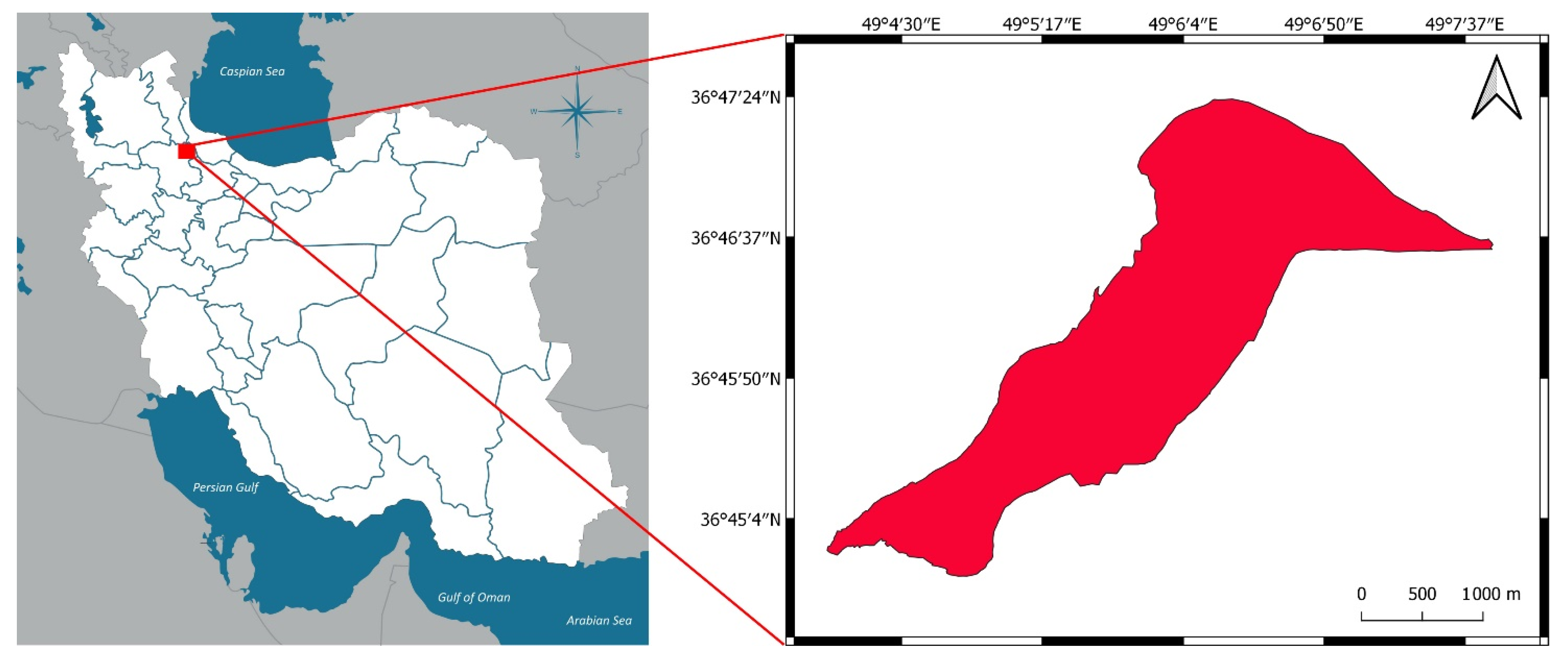
2.1. Study Area

This research was carried out in Tarom City (Zanjan Province), Iran, which has a wide range of climates (Figure 2). The semiarid cold climate, which occupies about 34% of the city area and, unlike the cold and humid climate, has the lowest location, is the driest. The region’s lowest point is 300 m above sea level, and the region’s highest point is 2700 m in the northeastern mountainous areas. Tarom receives 450 mm of annual rainfall on average, ranging from 200 mm in the lowlands to 1050 mm in the northern highlands. The average annual temperature is 17.3 degrees Celsius, with lows of 11 degrees Celsius and highs of 45 degrees Celsius. Autumn and spring are the rainiest seasons.

2.2. Field Data

Separately from agricultural and horticultural crops, the area under cultivation and the type of crop harvested were extracted from statistics from the Ministry of Jihad Agriculture and the Agricultural Jihad Organization of Zanjan region, as well as face-to-face interviews with Jihad Agricultural experts. More than 92,000 hectares of agrarian land will be covered by the agricultural sector with the cultivation of 68 types of crops and 21 types of horticultural crops in the region, and the volume of runoff produced by the region amounting to 2.2 billion cubic meters, which was constructed by several large and small dams or is under construction soon.

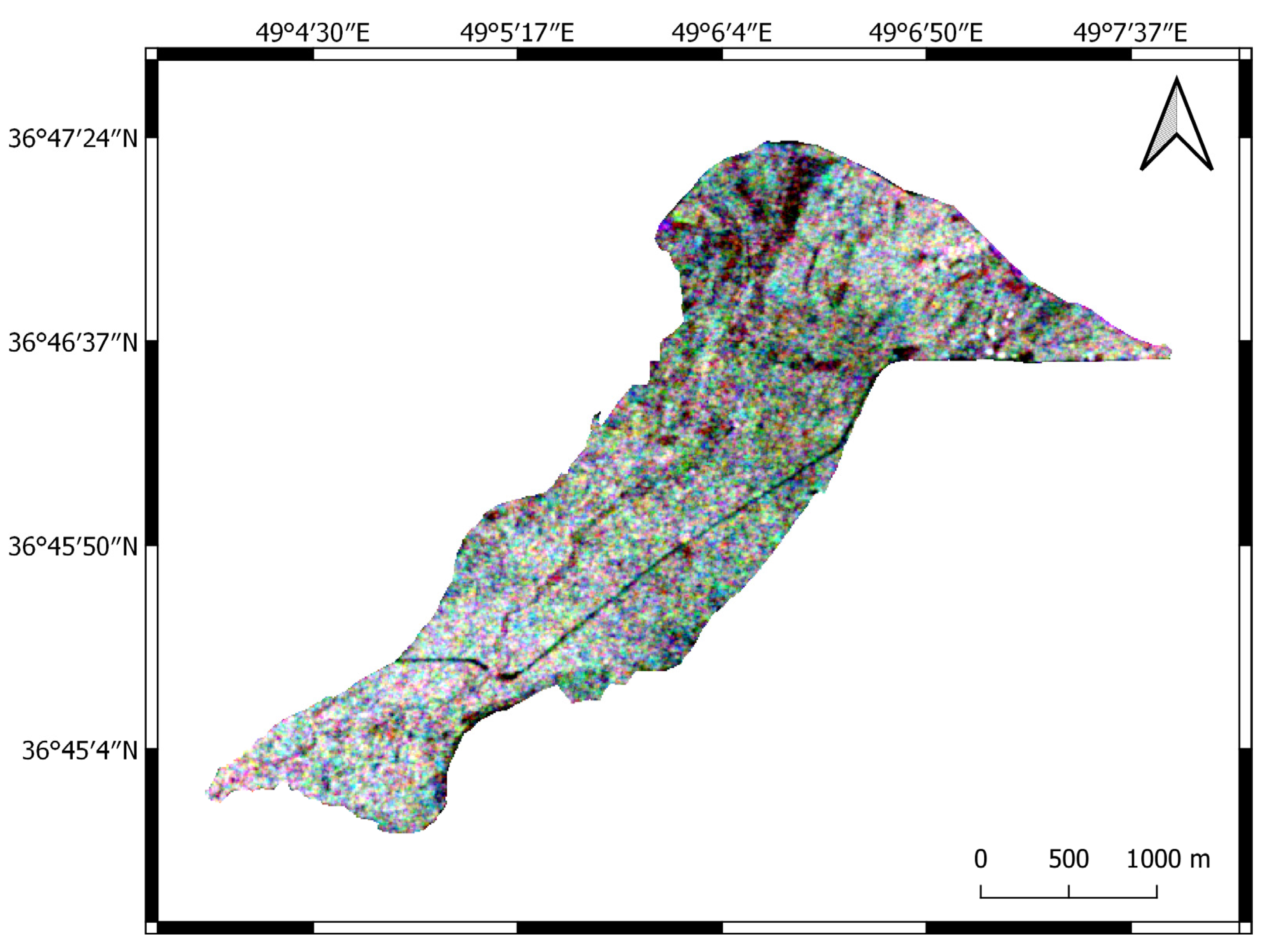
2.3. Sentinel 1 Data

The Sentinel 1 data came from Google Earth Engine’s (GEE) Level 1 Ground Range Detected (GRD) Interferometric Wide Swath (IW) product [20]. Sentinel 1 radar observations were projected onto a standard 10-m grid in GRD output. GEE preprocessed the data with the Sentinel 1 toolbox. Thermal noise reduction, radiometric calibration, and terrain correction were all part of the preprocessing. Sentinel 1’s key characteristics were the VV and VH polarized backscatter readings (in decibels, dB). The orientation of the transmitted radar beam has a significant impact on backscatter. Because of the considerably varied viewing orientations of the ascending and descending satellite overpasses, these were split and treated as supplementary observations. We used an improved Lee filter (Lee, 1981) with a damping value of 1 and a kernel size of 7 × 7 to minimize radar speckle in the pictures (Figure 3). To avoid the influence of changes in the angle of incidence on the return values, we employed two methods:

Ignore any observations with incidence angles less than 32° or greater than 42° because their geometries differed too much from the average incidence angle in our region of 37°. According to Equation (1), the remaining backscatter values observed at the angle of incidence θ are converted to backscatter values viewed at a reference angle ${\theta }_{ref}$ (1).

$${\sigma }_{{\theta }_{ref}}^0-\frac{{\sigma }_{\theta }^{0}co{s}^2\left({\theta }_{ref}\right)}{co{s}^2\left(\theta \right)}$$

(1)

In this equation, ${\sigma }_{\theta }^0$ is the measured incidence angle θ backscatter intensity, and ${\sigma }_{\theta re}^0$ is the predicted backscatter intensity under a reference angle ${\theta }_{ref}$ of 37 °C. This simplified adjustment was based on Lambert’s law of optics and assumed scattering processes. According to Lambert’s law, an ideal Lambert’s reflector reflects the quantity of light equal to the cosine of the angle of incidence of the radiation source in any direction; hence, according to this rule and for our categorization, the earth’s surface is not an ideal Lambert’s reflector. After the severe incidence angle was covered, two to five statements were recorded for each location over 12 days, resulting in a 12-day return mosaic from the combined visits of Sentinel 1A and Sentinel 1B. Because each satellite has a 12-month repeat visit, after the severe incidence angle was covered, two to five statements were recorded for each location over 12 days. All recorded backscatter values inside the 12-day window for each pixel were transformed from their dB values to the original values, averaged, and converted back to the 12-day mosaic backscatter values in dB.

2.4. Sentinel 2 Data

The Sen2Cor method [21] was used to mask for clouds and cloud shadows the Sentinel 2 Level-1C data from the Copernicus Open Access Hub, and then the iCOR atmospheric correction scheme [22] was used to atmospherically correct the data. An extra geometric adjustment based on manually determined ground control points was performed on Sentinel 2 scenes that were badly coregistered (i.e., had a multitemporal coregistration error of >0.5 pixels). At a spatial resolution of 10-m, we utilized the NDVI value derived from the red (B4) and near-infrared (B8) bands [23]. The NDVI measure was chosen as a typical optical descriptor because of its past effectiveness in crop categorization studies [20]. While NDVI was reported to saturate during the most productive parts of the growing season [24], utilizing this index in time series rather than single-date images was proven to overcome this problem. The categorization algorithm used these NDVI values as input. However, crop categorization over a wide area encompassing many image tiles is complicated by frequent and uniform cloud cover. An improved version of a pixel-wise weighted least-squares smoothing of the NDVI data over time [25] was used to eliminate cloud blockage. Between 1 March 2020, and 31 August 2020, smoothed NDVI images were created at 10-day intervals.

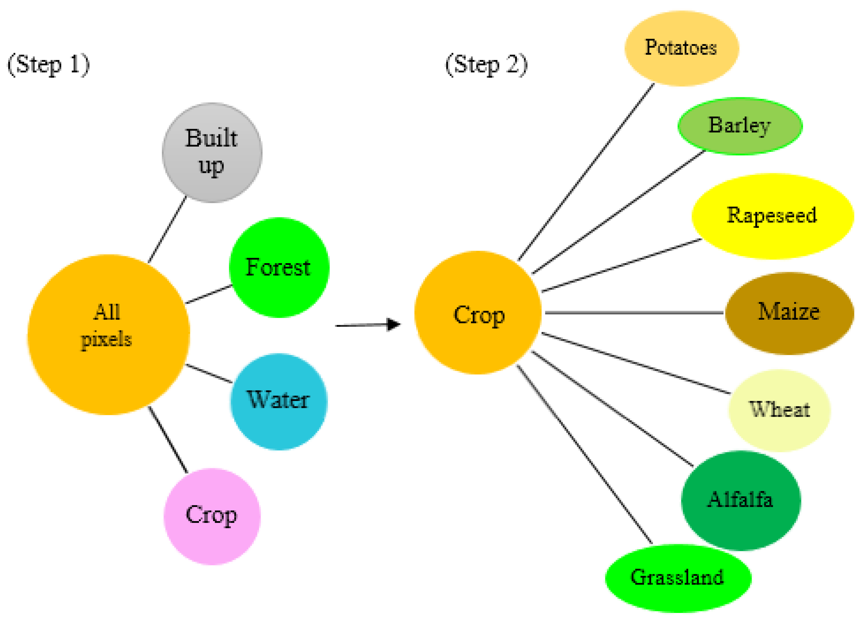
2.5. Classification of Hierarchical Random Forest

The decision tree is one of the most effective tools for estimating target variables or classifying patterns. A decision tree divides the input space into sections and assigns a response value to each section [25]. In simple terms, the average of the target values related to the patterns in each area can be used to determine the answer in regression problems, or, in other words, the responsibilities assigned to each area based on the average of the target values corresponds to the learning patterns in each area. RF is a new development method for decision trees that uses grounded rules to combine the predictions of several single algorithms. To create each tree, a different set of existing patterns is chosen, with each fixed design being replaced. The total number of available ways [26] will be used to determine the size of this chosen category. Because it performs better in research with extensive input data and various features, and estimates the purposes required for mapping, the RF algorithm is much more efficient than other classification models, such as neural networks. We use a unique process called bootstrapping in the random forest method. Each tree in this method represents one of the training samples that is chosen at random, and sub-branches in each of these trees are treated as a random set of input features. As can be seen in Figure 4, the classification method was broken down into two stages. The first stage involved creating classes, determining water and forest crop classes, and the second stage involved classifying the crops studied in this study. The appropriate network parameters are determined by the search in the random forest method. The minimum sample size required for a leaf node, the minimum sample size required to divide a node, the impurity criterion, and the number of trees are examples of these parameters.

The RF algorithm falls under the ensemble learning methods, in which multiple decision trees (forming a random forest) are built during training, after which the mode of the predicted classes of the individual trees forms the output class of the forest. The RF classifier usually outperforms simple decision trees due to less over-fitting. The random forest is constructed using a bootstrapping technique in which each tree is fitted based on a random subset of training samples with replacement, while at each split in this tree, a random subset of the input features is also selected. The classification method was divided into two different stages, the first stage including classes made, and water and forest with crop classes were determined, and in the second stage, the classification of crops studied in this research was done. In the random forest method, the appropriate parameters of the network are determined by the search. These parameters can be defined as the minimum sample size needed for a leaf node, the minimum sample size required to divide a node, the impurity criterion, and the number of trees [27].

2.6. Calibration and Validation Data

The data in the database were randomly divided into a set of 80% validity and 20% calibration, the purpose of which was to examine the percentage of data calibration and validation, and it was also considered that the final value in this range is not much different from the actual amount of data. For water-based, human-made, and forest-created classes, manual and training sets are generated, and the 20–80 division rule is used to capture all data. Subsets were considered in plots over 2 ha. In this study, both validation methods, calibration, and classification were based on pixels, and the buffer operation was not performed on validation. Due to the omission of small strings in training and different field sizes, a marked difference was observed between the pixel ratio and the initial verification and calibration ratio with the independent validation sample (

Table 1. Calibration and validation parcels and pixels per class.

Code	Class	Calibration Parcels	Validation Parcels	Calibration Pixels	Validation Pixels
1	Potatoes	613	5522	121,884	3,867,261
2	Barley	175	1590	31,189	1,333,238
3	Rapeseed	10	77	1520	50,159
4	Maize	1894	17,063	293,880	15,614,296
5	Wheat	848	7652	171,864	5,700,540
6	Alfalfa	352	3179	73,059	1,913,304
7	Grassland	2614	23,549	322,425	21,200,420
-	Total	7567	67,481	1,426,520	56,515,322

).

2.7. Classification Schemes

The main goal of this study was to determine the stock of individual and composite optical and SAR pictures in terms of classification accuracy. Furthermore, objective insight into the evolution of classification accuracy throughout the course of the growing season gives important information about the predicted accuracy of a classification during a certain phase of the growth season. One of the essential goals of this research is to compare SAR and optical images alone and the combination of these two in the classification process, and during the growing season we will find out the accuracy of classification with the help of these two images, and we can even comment on the accuracy of the classification with the help of these images in a certain period. According to

Table 2. Overall accuracy (OA) and kappa coefficient (k) of various categorization plans.

			Sentinel 2					Sentinel 1
#	March	April	May June	July	August	March	April	May June	July	August	OA	κ
1						X					0.44	0.33
2						X	X				0.60	0.52
3						X	X	X			0.72	0.61
4						X	X	X  X			0.73	0.70
5						X	X	X  X	X		0.72	0.64
6						X	X	X  X	X	X	0.78	0.70
7	X										0.42	0.30
8	X	X									0.56	0.42
9	X	X	X								0.70	0.57
10	X	X	X  X								0.73	0.65
11	X	X	X  X	X							0.74	0.72
12	X	X	X  X	X	X						0.80	0.73
13	X					X					0.55	0.42
14	X	X				X	X				0.67	0.57
15	X	X	X			X	X	X			0.74	0.67
16	X	X	X  X			X	X	X  X			0.81	0.74
17	X	X	X  X	X		X	X	X  X	X		0.83	0.80
18	X	X	X  X	X	X	X	X	X  X	X	X	0.84	0.79

, 18 classification designs were determined. Sentinel 1 SAR images were used only for the first six designs, Sentinel 2 NDVI images for the second six designs, and Sentinel 1 and Sentinel 2 composite images for the third six designs. In all 18 classification schemes, the performance estimators were OA classification and Kappa Cohen (K) agreement coefficient. The following equation represents the OA calculation:

$$\mathrm{OA}=\frac{{{\displaystyle \sum }}^{}correct predictions}{total number of predictions}$$

(2)

In the Equation (2), the predictions are presented for all validation examples, the expected and real cases are comparable, and the following equation representing the K calculation is also used:

$$\mathrm{K}=\frac{p_0-p_e}{1-p_e}$$

(3)

where p₀ is the relative observed agreement among raters, and p_e is the hypothetical probability of chance agreement.

2.8. Classification Accuracy

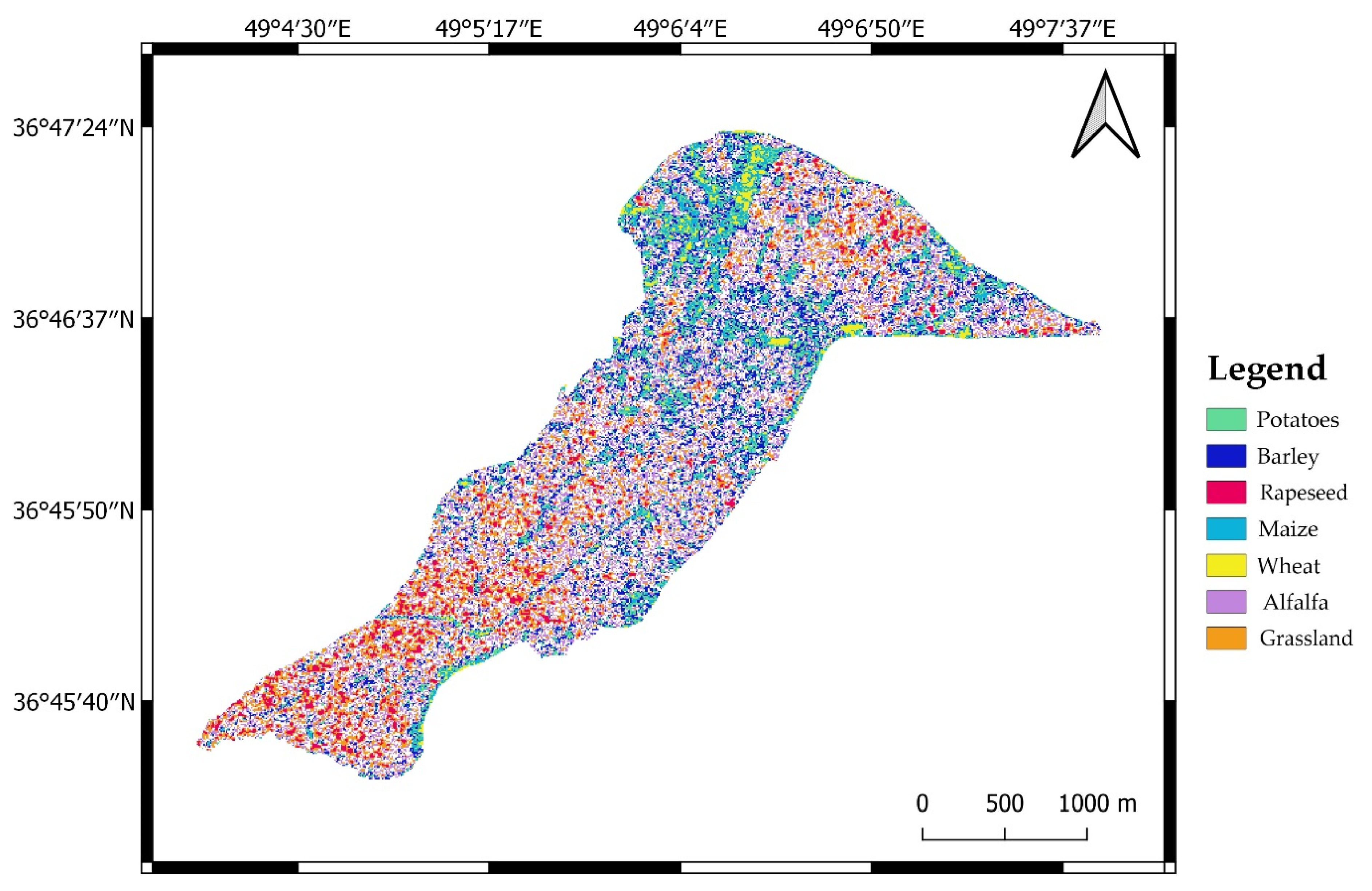
Estimating the purpose of the classification, the random forest classification method is also used to predict the classification accuracy, and the average probability of the expected class of trees in the forest about the possibilities of the predicted class is an input sample. The probability of a winning class is defined based on the classification certainty for a particular instance. More reliable classification and strong agreement between different trees indicate high accuracy, but disagreement between trees reduces the likelihood of predicting a reliable classification. The prediction result will be shown at the pixel- or sample-level [28].

3. Result

The trend of changes in the two variables kappa and OA in the classification methods in this study is shown in the following table (Table 2). The table shows that as the number of images used as input values grows, so do the values of the two variables kappa and OA. Controlling the degree of resolution of the categories and the differences between the types of crops can be used to investigate this increase. The differences between Sentinel 1 and Sentinel 2 and optical classification versus SAR classification can be analyzed by examining the results.

Sentinel 1 classification performed better than Sentinel 2 classification in March. Moreover, the optical-only classification performed better than the SAR-only classification throughout the growing season (kappa of 0.69 vs. 0.67, OA of 77 percent vs. 75 percent). According to these findings, different crops in early growth have different characteristics that can be detected and compared with the light spectrum, but this conclusion can only be applied to the crops studied in this study, such as winter cereals. Optical and radar signatures for crops grown in April and May, such as potatoes and corn, reveal the type of management method used and reflect the winter plant cover, which is difficult to distinguish between optical and radar studies. A combination of Sentinel 1 and Sentinel 2 images performs better than using a single sensor for classification. The maximum accuracy obtained in the last days of July was 81 percent, which could not be increased by combining with August images. Figure 5 depicts the final classification as of the last day of August 2020. For this purpose, no filtration was used, and the image’s recognizability is the result of the classification packages in the crop area’s landscape. Due to the similarity between alfalfa and potatoes at the start of the growing season, all crops were classified as potatoes at first, but with time and growth evolution, this error was eliminated in the last days of August, and the distinction between alfalfa and potato was evident in the crop classification.

Figure 6 shows the results, where certain within-field zones in the center field, which is part of the validation dataset, were incorrectly classified as alfalfa in the early mapping stage (taken here in June 2020) but were correctly identified as potato by the end of August. Figure 6 was specified to eliminate this ambiguity with two letters (a) and (b). At the beginning of June 2020, the whole crop was identified as alfalfa in the study area due to the phenological similarities between the two crops of alfalfa and potatoes and the lack of development of plant growth, but at the end of August, due to full plant growth and obvious phenological differences, it was possible to distinguish between the two crops (purple represents alfalfa, and green represents potatoes).

Figure 7 depicts the classification result’s dependability. Because the side pixels are due to the integration with the signals of the surrounding terrain, the data have low validity along the considered boundaries. Figure 7 shows the results for the high data invalidity at the pixel boundary, which is close to the central packet. Wheats were the crops grown in this package, but the data uncertainty can be seen in the central portion of the packages, which can be attributed to the inconsistency created in the pixels’ background.

To ensure classification performance, which is a function of classification reliability, the method of quantifying classification accuracy was used. To accomplish this, all samples will be used, all data will be validated, the RF classifier will be used, and all samples will be averaged at a certain level. In terms of Gini, this function calculates the characteristics of the input data. The significance of the two radar and optical input sources’ characteristics must be examined in the data [29]. We use the Gini significance feature as a reduction of impurities when using the random forest classifier, which is used for all forest trees. Gini’s personality is extremely valuable. Its high importance indicates that it plays a key role in the forecasting process; on the other hand, if the feature’s importance is low, it means that, according to Sentinel 1 sensor data, this information was limited for prediction before May, despite being consistent with plant structure. Early April and May play a critical role in the longitudinal development of winter crops and the ability to distinguish summer crops from one another. Plant development shows a difference in their NDVI values over time and during the growing season. Changes in the amount of NDVI will cause plants to differentiate due to differences in their phenological structure. This distinction is particularly noticeable between July and August, when the crops are distinguishable from one another due to growth and development.

4. Discussion

If we want to correctly classify crops in a region, we need to concentrate on the uniformity of all available inputs. If the data is related to Sentinel 1 data, 12-day return mosaics can be created. It is crucial to be cautious when it comes to reducing the impact of angles on the output data. We need to use a filter to get high-quality and high-resolution radar images. The Lee filter is one of the most comprehensive filters for this situation. The sharpness of radar images is reduced due to blurry effects. Twelve-day return mosaics and time series can be used to compensate for this flaw, and this annoying effect can be easily removed or reduced using this technique. However, because the classification was not the main criterion in terms of time, this disorder will not cause a primary problem, according to the method used in this study. Quegan et al. [30] used a special time filter in their study that could be considered a new method, but using their method was not a priority in this study. For Sentinel 2 data, this method was used to smooth out all cloud effects in NDVI images, and 10-day NDVI mosaics were considered without cloud and fog coverage. When all predicting classes in one step lead to a 1.5 percent increase in the OA index in Tarom for mapping crops using random forest hierarchical and time-series model inputs, the results showed that the method of two-step hierarchical use of the method is nonhierarchical.

The first classification step was completed in August, with an OA index of around 84 percent due to differences in radar and optical effects for three different crops (forest, construction, water). The random forest method can be used in the second stage to identify more specialized differences between classes. During rejection, significant increases in both kappa and OA were reported, though by the end of May, summer crops (potatoes and corn) had grown significantly, but winter crops had also grown significantly. Increased classification accuracy will result from increased awareness of crop phenological development stages. Previous research has demonstrated that the use of optical time series improves the principles of classification by allowing for the separation of crops [31]. Separation of crops, such as cereals and vegetable crops, as well as winter and summer crops, is strongly recommended to improve the quality of classification work, despite the difficulties that such separation poses due to the similarity of crops such as winter wheat and winter barley. To solve the problem, it is suggested that winter crops be classified alongside summer crops. It is difficult to separate grasslands from winter crops (cereals) and winter crops from summer crops. Making a classification error between grassland and winter crops can be explained by the fact that both of these crops grow well in the months of April and May, and the green mass is visible on both crops, making it difficult to distinguish between them. Furthermore, vegetable crops such as potatoes and corn are very similar to one another until the end of plant growth, making it difficult to separate them by the end of April in practice. This can be thought of as a drawback to using remote sensing for such purposes.

Given the high values of the two kappa and OA indices during the study period (growth season), the items obtained as a result become more citational over time, but the results cannot be obtained in a specific time frame. As a result, it is important to remember that we will have to wait a certain amount of time to get the desired and required results from the crops for classification, because the variables in this study are crops that require time, and a set of observations takes time to evolve. One of the study’s most important findings is that the difference in the OA variable for the classification process at the start of the growing season using two sensors, Sentinel 1 and Sentinel 2, revealed that this index (OA) was higher in studies using Sentinel 1. The difference between the use of Sentinel 1 and Sentinel 2 sensors will be determined after 30 days of the growing season, so that the data as predictor variables from these two sensors will be significantly different. The characteristics of the input data can be attributed to the greater validity of radar data for the crop classification process. The values of the OA variable were 35 percent lower when the analyses were done solely with VH backscatter, which was even lower than when the analyses were done with Sentinel 2 NDVI. On the basis of this evidence, it is impossible to say with certainty that the radar results differ from the optical classification of the first months of the growing season.

One of the issues with classifications that rely solely on optical methods is the use of a predictor variable, which is frequently the NDVI predictor. Previous research [31] focused on this factor, but it was later determined that NDVI could not provide a complete view of Sentinel 2 optical images, so it is recommended that more bands be used to achieve a more comprehensive view of optical images [32]. The method described in Section 2.5 does not apply to the NDVI index or single spectral bands. Although the use of different optical indices is recommended for future research, the focus of this study is on the use of a valid vegetation index (10-m resolution NDVI). The use of radar data, such as interferometry coherence stacks [33], can improve the validity of the classification process. Future research should consider whether classification based on radar data is more accurate than classification based on optical data. In the growing season, this case can answer the research hypothesis that radar data is more efficient than cloud position.

This study found that two periods are more important for classification when using the NDVI predictor variable. Winter crops grew the most longitudinally in May and April, and it was during this time that summer crops began to grow, making it possible to classify bare soil and other plants with summer crops. Due to the clear sky and lack of clouds during this time, optical images can be obtained in greater detail. August and July are the two most important months for making more use of sunlight. The winter grain harvest season and greater access to summer crops in the summer are two other factors that aid in the sorting process. According to Zhou et al. [18], the VV index takes precedence over the HV index when classifying crops, but we found no difference in the classification process between the two variables in this study.

NDVI is the most important predictor when considering the characteristics of Sentinel 1 and Sentinel 2, as well as their ability to estimate forecasts. The most important crop classification predictions are made using a combination of radar and optical features. The accuracy of classification in areas close to the center is greater than the accuracy of classification at pixel borders when it comes to crop classification at the pixel level. The data are all qualitative, indicating a close relationship between classification accuracy and classification reliability, but statistical probability cannot be used to estimate the percentage of reliability, and statistics was ineffective in this study when it came to crop classification.

The results of this study showed that using Sentinel 2 optical data as a supplement to Sentinel 1 SAR data provided comprehensive information on plant structure [34]. Furthermore, by using time-series images rather than single images, the problem of determining the date of the images is eliminated [35]. High-accuracy results were reported in several studies that used a combined method of optical and radar images. The reason for this is that in some studies, the classification performed was related to the level [36], or filtration was used in the classification [31], but in this study, the unfiltered method of classification in pixels was used in addition to a small amount of OA. It is difficult to group similar crops together, but if we look into several specific classes of different crops, the accuracy of crop classification will improve. This obvious difference in the structure of plants will facilitate classification if the plants are classified in terms of structure and family [37,38], such as the classification of horticultural and agricultural crops [39], paddy and grassland. The findings of our study are in line with those of previous studies. Data and their properties can be prioritized over pixels in such studies, allowing the data from the two sensors Sentinel 1 and Sentinel 2 to be used as input. Closed space can also be used with the classification method, which has the advantage of lowering the signal-to-noise ratio. We can look into the differences between radar and optical data, spectroscopic interference, optical image SWIR bands, and plant phenological differences as one of the input factors for classification in the future.

5. Conclusions

The need to feed the population is prioritized as a result of population growth. Identification of high-consumption crops and their alternative varieties is one of the main issues in future planning to meet the nutritional needs of large-scale crop cultivation. Supplying the cultivated crop’s fertilizer needs, awareness of water needs, and early detection of anomalies are all critical in the second stage. These issues were largely solved by new technologies such as remote sensing and the use of satellite imagery. When compared to that of traditional classification methods, the Copernicus program develops the potential for classification through the simultaneous use of multiple sensors. The classification accuracy was said to improve with the combination of radar data and optical signals in previous studies because one of the benefits of combining these data is that the cloud effect is reduced. We used 10-day Sentinel 2 smoothed NDVI mosaics and 12-day Sentinel 1 back mosaics to create a classification map for the 2020 growing season in Tarom. The random forest method was used for classification purposes. This study reported a kappa coefficient of 0.75 and a maximum accuracy of 85 percent. It is recommended to use a combination of radar and optical data to achieve maximum classification accuracy, as this combination will increase the chances of examining the details compared to a single-sensor classification method and provide more reliable information. This study found that combining optical and radar data was the most important factor in predicting the final classification, and that using optical data alone produced acceptable results. Finally, because the level of reliability is low in areas such as closed border areas, it is much more difficult to predict the classification than to give a general conclusion using such methods. It is also necessary to compare the results of various sensors to better assess their ability to classify crops and to assess the potential of various sensors for such research.

References

1. Jain, M.; Balwinder-Singh; Rao, P.; Srivastava, A.K.; Poonia, S.; Blesh, J.; Azzari, G.; McDonald, A.J.; Lobell, D.B. The impact of agricultural interventions can be doubled by using satellite data. Nat. Sustain. 2019, 2, 931–934. [Google Scholar] [CrossRef]
2. Sharifi, A. Estimation of biophysical parameters in wheat crops in Golestan province using ultra-high resolution images. Remote Sens. Lett. 2018, 9, 559–568. [Google Scholar] [CrossRef]
3. Kosari, A.; Sharifi, A.; Ahmadi, A.; Khoshsima, M. Remote sensing satellite’s attitude control system: Rapid performance sizing for passive scan imaging mode. Aircr. Eng. Aerosp. Technol. 2020, 92, 1073–1083. [Google Scholar] [CrossRef]
4. Wu, F.; Wu, B.; Zhang, M.; Zeng, H.; Tian, F. Identification of crop type in crowdsourced road view photos with deep convolutional neural network. Sensors 2021, 21, 1165. [Google Scholar] [CrossRef]
5. Van Tricht, K.; Gobin, A.; Gilliams, S.; Piccard, I. Synergistic use of radar sentinel 1 and optical sentinel 2 imagery for crop mapping: A case study for Belgium. Remote Sens. 2018, 10, 1642. [Google Scholar] [CrossRef] [Green Version]
6. Ghaderizadeh, S.; Abbasi-Moghadam, D.; Sharifi, A.; Zhao, N.; Tariq, A. Hyperspectral Image Classification Using a Hybrid 3D-2D Convolutional Neural Networks. IEEE J. Sel. Top. Appl. Earth Obs. Remote Sens. 2021, 14, 7570–7588. [Google Scholar] [CrossRef]
7. Sharifi, A.; Amini, J.; Sumantyo, J.T.S.; Tateishi, R. Speckle reduction of PolSAR images in forest regions using fast ICA algorithm. J. Indian Soc. Remote Sens. 2015, 43, 339–346. [Google Scholar] [CrossRef]
8. McNairn, H.; Brisco, B. The application of C-band polarimetric SAR for agriculture: A review. Can. J. Remote Sens. 2004, 30, 525–542. [Google Scholar] [CrossRef]
9. Baillarin, S.J.; Meygret, A.; Dechoz, C.; Petrucci, B.; Lacherade, S.; Tremas, T.; Isola, C.; Martimort, P.; Spoto, F. Sentinel 2 level 1 products and image processing performances. In Proceedings of the 2012 IEEE International Geoscience and Remote Sensing Symposium, Munich, Germany, 22–27 July 2012; pp. 7003–7006. [Google Scholar] [CrossRef] [Green Version]
10. Sharifi, A. Development of a method for flood detection based on Sentinel 1 images and classifier algorithms. Water Environ. J. 2020, 35, 924–929. [Google Scholar] [CrossRef]
11. Uddin, K.; Matin, M.A.; Meyer, F.J. Operational flood mapping using multi-temporal Sentinel 1 SAR images: A case study from Bangladesh. Remote Sens. 2019, 11, 1581. [Google Scholar] [CrossRef] [Green Version]
12. McNairn, H.; Champagne, C.; Shang, J.; Holmstrom, D.; Reichert, G. Integration of optical and Synthetic Aperture Radar (SAR) imagery for delivering operational annual crop inventories. ISPRS J. Photogramm. Remote Sens. 2009, 64, 434–449. [Google Scholar] [CrossRef]
13. Soria-Ruiz, J.; Fernandez-Ordońez, Y.; Woodhouse, I.H. Land-cover classification using radar and optical images: A case study in Central Mexico. Int. J. Remote Sens. 2010, 31, 3291–3305. [Google Scholar] [CrossRef]
14. Inglada, J.; Vincent, A.; Arias, M.; Marais-Sicre, C. Improved early crop type identification by joint use of high temporal resolution sar and optical image time series. Remote Sens. 2016, 8, 362. [Google Scholar] [CrossRef] [Green Version]
15. Ferrant, S.; Selles, A.; Le Page, M.; Herrault, P.A.; Pelletier, C.; Al-Bitar, A.; Mermoz, S.; Gascoin, S.; Bouvet, A.; Saqalli, M.; et al. Detection of irrigated crops from Sentinel 1 and Sentinel 2 data to estimate seasonal groundwater use in South India. Remote Sens. 2017, 9, 1119. [Google Scholar] [CrossRef] [Green Version]
16. Joshi, N.; Baumann, M.; Ehammer, A.; Fensholt, R.; Grogan, K.; Hostert, P.; Jepsen, M.R.; Kuemmerle, T.; Meyfroidt, P.; Mitchard, E.T.A.; et al. A review of the application of optical and radar remote sensing data fusion to land use mapping and monitoring. Remote Sens. 2016, 8, 70. [Google Scholar] [CrossRef] [Green Version]
17. De Oliveira Pereira, L.; Da Costa Freitas, C.; Anna, S.J.S.S.; Lu, D.; Moran, E.F. Optical and radar data integration for land use and land cover mapping in the Brazilian Amazon. GIScience Remote Sens. 2013, 50, 301–321. [Google Scholar] [CrossRef]
18. Zhou, T.; Pan, J.; Zhang, P.; Wei, S.; Han, T. Mapping winter wheat with multi-temporal SAR and optical images in an urban agricultural region. Sensors 2017, 17, 1210. [Google Scholar] [CrossRef] [PubMed]
19. Campos-Taberner, M.; García-Haro, F.J.; Camps-Valls, G.; Grau-Muedra, G.; Nutini, F.; Busetto, L.; Katsantonis, D.; Stavrakoudis, D.; Minakou, C.; Gatti, L.; et al. Exploitation of SAR and optical sentinel data to detect rice crop and estimate seasonal dynamics of leaf area index. Remote Sens. 2017, 9, 248. [Google Scholar] [CrossRef] [Green Version]
20. Bellón, B.; Bégué, A.; Seen, D.L.; de Almeida, C.A.; Simões, M. A remote sensing approach for regional-scale mapping of agricultural land-use systems based on NDVI time series. Remote Sens. 2017, 9, 600. [Google Scholar] [CrossRef] [Green Version]
21. De Keukelaere, L.; Sterckx, S.; Adriaensen, S.; Knaeps, E.; Reusen, I.; Giardino, C.; Bresciani, M.; Hunter, P.; Neil, C.; Van der Zande, D.; et al. Atmospheric correction of Landsat-8/OLI and Sentinel 2/MSI data using iCOR algorithm: Validation for coastal and inland waters. Eur. J. Remote Sens. 2018, 51, 525–542. [Google Scholar] [CrossRef] [Green Version]
22. Zheng, B.; Myint, S.W.; Thenkabail, P.S.; Aggarwal, R.M. A support vector machine to identify irrigated crop types using time-series Landsat NDVI data. Int. J. Appl. Earth Obs. Geoinf. 2015, 34, 103–112. [Google Scholar] [CrossRef]
23. Rouse, W.; Haas, R.H.; Schell, J.A.; Deering, D.W. Monitoring vegetation systems in the Great Plains with ERTS. NASA Spec. Publ. 1974, 351, 309. [Google Scholar]
24. Cai, Y.; Guan, K.; Peng, J.; Wang, S.; Seifert, C.; Wardlow, B.; Li, Z. A high-performance and in-season classification system of field-level crop types using time-series Landsat data and a machine learning approach. Remote Sens. Environ. 2018, 210, 35–47. [Google Scholar] [CrossRef]
25. Estel, S.; Kuemmerle, T.; Alcántara, C.; Levers, C.; Prishchepov, A.; Hostert, P. Mapping farmland abandonment and recultivation across Europe using MODIS NDVI time series. Remote Sens. Environ. 2015, 163, 312–325. [Google Scholar] [CrossRef]
26. Ouyang, F.; Su, W.; Zhang, Y.; Liu, X.; Su, J.; Zhang, Q.; Men, X.; Ju, Q.; Ge, F. Ecological control service of the predatory natural enemy and its maintaining mechanism in rotation-intercropping ecosystem via wheat-maize-cotton. Agric. Ecosyst. Environ. 2020, 301, 107024. [Google Scholar] [CrossRef]
27. Belgiu, M.; Drăgu, L. Random forest in remote sensing: A review of applications and future directions. ISPRS J. Photogramm. Remote Sens. 2016, 114, 24–31. [Google Scholar] [CrossRef]
28. Sharifi, A.; Amini, J.; Tateishi, R. Estimation of forest biomass using multivariate relevance vector regression. Photogramm. Eng. Remote Sens. 2016, 82, 41–49. [Google Scholar] [CrossRef] [Green Version]
29. Snapp, S.; Bezner Kerr, R.; Ota, V.; Kane, D.; Shumba, L.; Dakishoni, L. Unpacking a crop diversity hotspot: Farmer practice and preferences in Northern Malawi. Int. J. Agric. Sustain. 2019, 17, 172–188. [Google Scholar] [CrossRef]
30. Quegan, S.; Toan, T.L.; Yu, J.J.; Ribbes, F.; Floury, N. Multitemporal ERS SAR analysis applied to forest mapping. IEEE Trans. Geosci. Remote Sens. 2000, 38, 741–753. [Google Scholar] [CrossRef]
31. Yan, S.; Shi, K.; Li, Y.; Liu, J.; Zhao, H. Integration of satellite remote sensing data in underground coal fire detection: A case study of the Fukang region, Xinjiang, China. Front. Earth Sci. 2020, 14, 1–12. [Google Scholar] [CrossRef]
32. Francini, S.; McRoberts, R.E.; Giannetti, F.; Mencucci, M.; Marchetti, M.; Scarascia Mugnozza, G.; Chirici, G. Near-real time forest change detection using PlanetScope imagery. Eur. J. Remote Sens. 2020, 53, 233–244. [Google Scholar] [CrossRef]
33. Shanmugapriya, S.; Haldar, D.; Danodia, A. Optimal datasets suitability for pearl millet (Bajra) discrimination using multiparametric SAR data. Geocarto Int. 2020, 35, 1814–1831. [Google Scholar] [CrossRef]
34. Moreau, D.; Pointurier, O.; Nicolardot, B.; Villerd, J.; Colbach, N. In which cropping systems can residual weeds reduce nitrate leaching and soil erosion? Eur. J. Agron. 2020, 119, 126015. [Google Scholar] [CrossRef]
35. Saleem, M.; Pervaiz, Z.H.; Contreras, J.; Lindenberger, J.H.; Hupp, B.M.; Chen, D.; Zhang, Q.; Wang, C.; Iqbal, J.; Twigg, P. Cover crop diversity improves multiple soil properties via altering root architectural traits. Rhizosphere 2020, 16, 100248. [Google Scholar] [CrossRef]
36. Muoni, T.; Koomson, E.; Öborn, I.; Marohn, C.; Watson, C.A.; Bergkvist, G.; Barnes, A.; Cadisch, G.; Duncan, A. Reducing soil erosion in smallholder farming systems in east Africa through the introduction of different crop types. Exp. Agric. 2019, 56, 183–195. [Google Scholar] [CrossRef] [Green Version]
37. Ahmad, A.; Ahmad, S.R.; Gilani, H.; Tariq, A.; Zhao, N.; Aslam, R.W.; Mumtaz, F. A synthesis of spatial forest assessment studies using remote sensing data and techniques in Pakistan. Forests 2021, 12, 1211. [Google Scholar] [CrossRef]
38. Burke, M.; Lobell, D.B. Satellite-based assessment of yield variation and its determinants in smallholder African systems. Proc. Natl. Acad. Sci. USA 2017, 114, 2189–2194. [Google Scholar] [CrossRef] [PubMed] [Green Version]
39. Li, G.; Messina, J.P.; Peter, B.G.; Snapp, S.S. Mapping land suitability for agriculture in Malawi. Land Degrad. Dev. 2017, 28, 2001–2016. [Google Scholar] [CrossRef]
Figure 1. Example of profiles of (upper panel) Sentinel 2 normalized difference vegetation index (NDVI) and (lower panel) Sigma0 VV and VH backscatter intensities for a winter wheat field.
Applsci 11 10104 g001
Figure 2. Location of the study area.
Applsci 11 10104 g002
Figure 3. Sentinel 1 VH backscatter mosaics from 12 days in RGB composite. Dates are 1–13 March 2020 (red), 17–29 June 2020 (green), and 16–28 August 2020 (blue).
Applsci 11 10104 g003
Figure 4. Schematic overview of two-step hierarchical classification procedure.
Applsci 11 10104 g004
Figure 5. Final categorization result based on Sentinel 1 and 2 inputs through August 2020.
Applsci 11 10104 g005
Figure 6. Zones in middle field were misclassified as alfalfa in June (a) but were correctly labeled as potato in August (b).
Applsci 11 10104 g006
Figure 7. Classification confidence defined as random forest predicted class probability of majority class for each pixel at end of August 2020.
Applsci 11 10104 g007