2.1. Participants
Four population groups including adults, adolescents, and children were identified to show the variations in the particular anthropometric dimensions taking the territorial difference into account. The anthropometric measurements were carried out on Czech adults, employees of the University of West Bohemia, Czech children, and Czech adolescents during sports activities. The total number of subjects was 152 ranging in age from 6 y to 56 y. The Chinese adults were employees of the Tianjin Technician Institute of Mechanical & Electrical Technology. Their total number was 68, ranging in age from 24 y to 60 y. The males and females were equally represented.
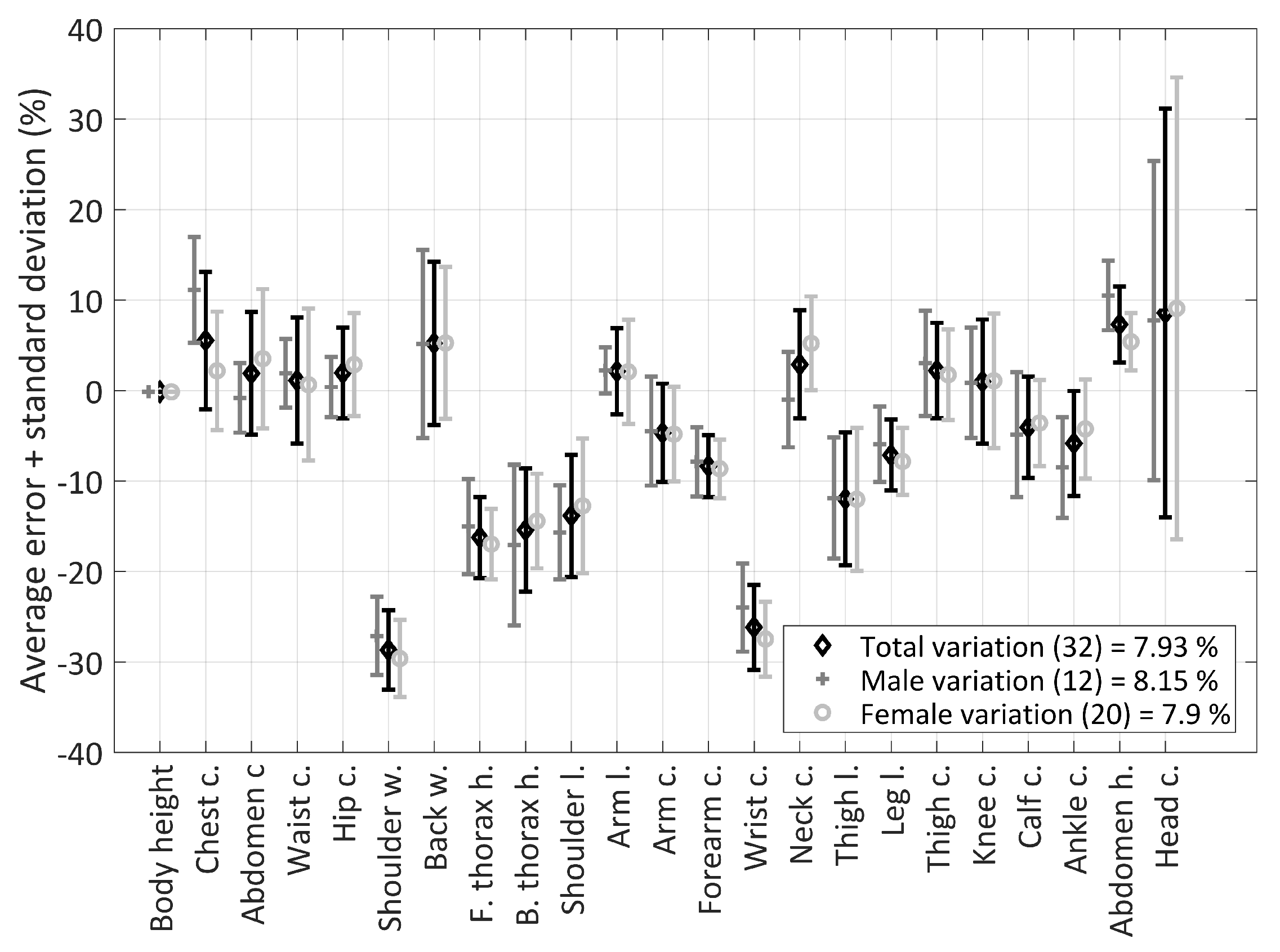
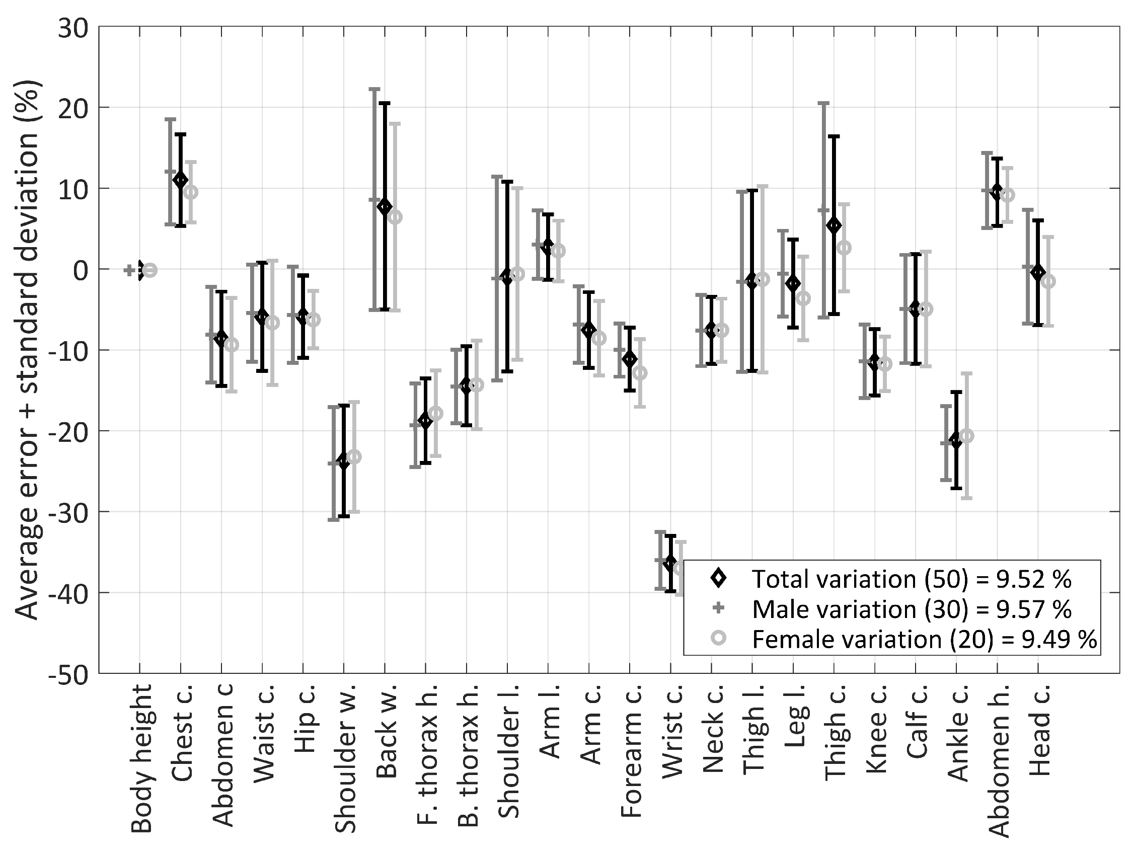
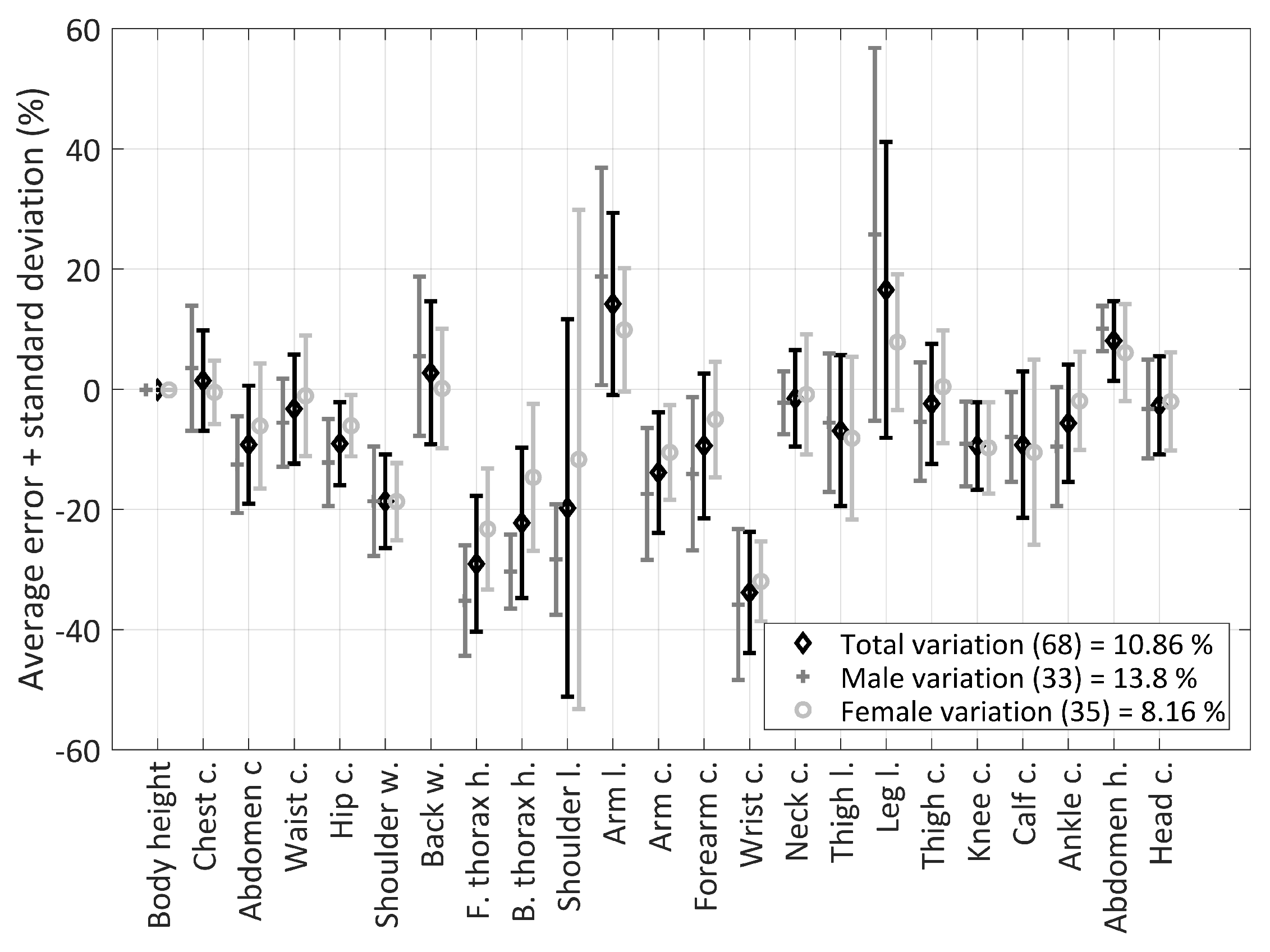
The measurements were carried out on adult students and adult employees (N = 70, of which 38 males and 32 females, aged between 20 y and 56 y, weight between 47 kg and 105 kg, and height between 159 cm and 193 cm) from the Faculty of Applied Sciences, the Faculty of Education, and the New Technologies—Research Centre, all three entities of the University of West Bohemia. The employees were members of the biomechanical team from the Faculty of Applied Sciences, the Faculty of Education, and the New Technologies—Research Centre at the University of West Bohemia, and the students were those participating in subjects related to biomechanics. Further, informed employees of the University of West Bohemia carried out the measurements on children (N = 50, of which 30 were boys and 20 girls, aged between 5.5 y and 7.5 y, weight between 18.3 kg and 35.6 kg, and height between 110 cm and 134 cm) from kindergartens cooperating with the Faculty of Education of the University of West Bohemia and on adolescents (N = 32, of which 12 were males and 20 females, aged between 10 y and 19 y, weight between 35 kg and 90 kg, and height between 144 cm and 188 cm) who were students or children of employees of the University of West Bohemia, during sports courses or at home. These children and adolescents participated in the regular sports courses under professional guidance by the physical education team from the Faculty of Education of the University of West Bohemia. Additional measurements were carried out on adult employees of the Tianjin Technician Institute of Mechanical & Electrical Technology (N = 68, of which 33 were males and 35 females, aged between 24 y and 60 y, weight between 49 kg and 110 kg, and height between 155 cm and 184 cm) in China at their workplaces, which were recruited from the teaching staff.
All recruitment was carried out on a voluntary basis. The Chinese participant were chosen in order to emphasize the anthropometric variations between populations from considerably different territories. All participants were measured wearing only underwear. The operators performing the measurements were instructed by the physical education experts from the Faculty of Education of the University of West Bohemia to ensure the accuracy and repeatability.
Table 1 summarizes the measured subjects involved in the study.
2.5. Personalization Algorithm
The personalization provided the local geometrical and biomechanical details of the human body. Firstly, the scaling [
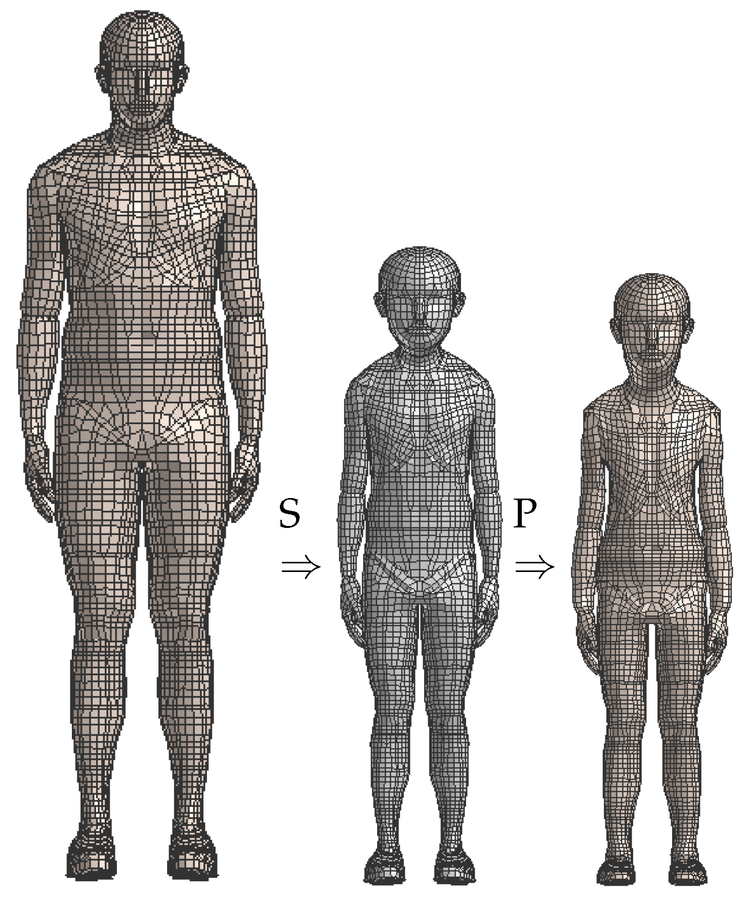
7] was performed for each subject to target the given gender, age, height, and weight. Having the scaled model, the personalization to provide the correct anthropometric dimensions was carried out. The two-step approach is described as:
meaning
T (target) equals
S (scaling) plus
P (personalization) where
describes the coordinates of any point of the subject-specific (target) model referring to the same point
in the reference model, which is firstly scaled to a semistate
in the scaled model.
refers to a spatial point in the global coordinate system with the origin in the H-point (the point in the middle between the hip joints) with the axis
x (defining the depth) pointing anteriorly to the front. The sagittal plane is the plane
(the axis
z defining the height points cranially to the head), and the axis
y (defining the width) is directed laterally from the right to the left forming the right-hand side system.
Personalization was the next step after scaling. Scaling is a necessary step to have a model with global dimensions for the particular human body size before applying the mathematical operation to refine the surface locally. As the scaling algorithm was published previously, this paper does not address it, referring to the work by Hynčík et al. [
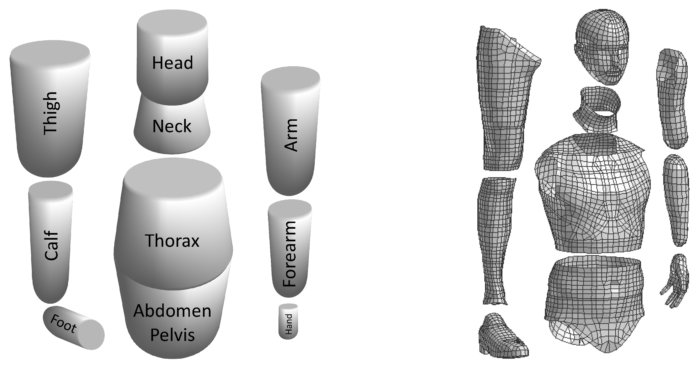
7]. For personalization purposes, the scaled model was divided into segments summarized in
Table 3 and schematically shown in
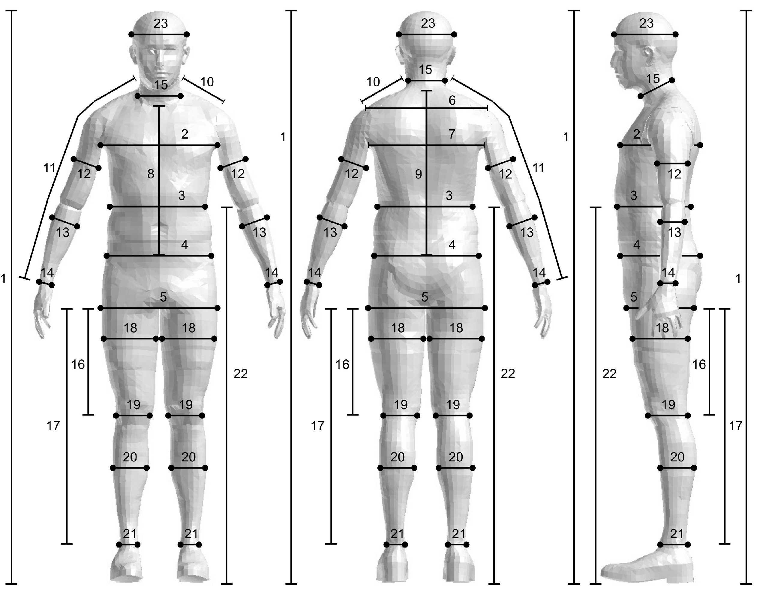
Figure 3. Each segment can be described by the anthropometric dimensions from
Table 2 displayed in
Figure 1. The personalization algorithm ran independently of each of the 16 subject-specific segments defined in
Table 3 using the corresponding dimensions from
Table 2. There was a reference node
chosen on each segment as a local coordinate system origin, against which it was personalized, which also served to connect the neighboring segments following the open-tree segment system in the multibody structure. This is usually the joint connecting the neighboring segments [
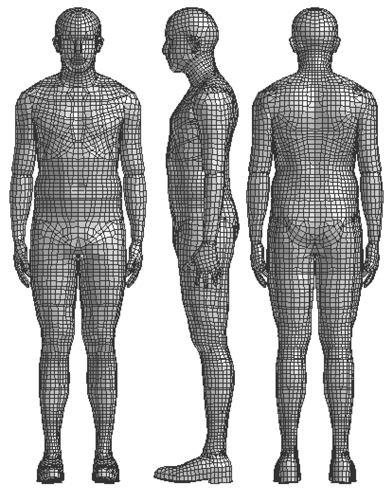
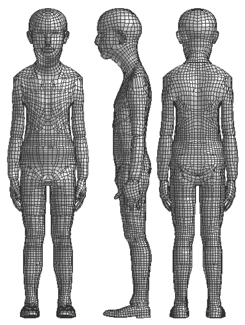
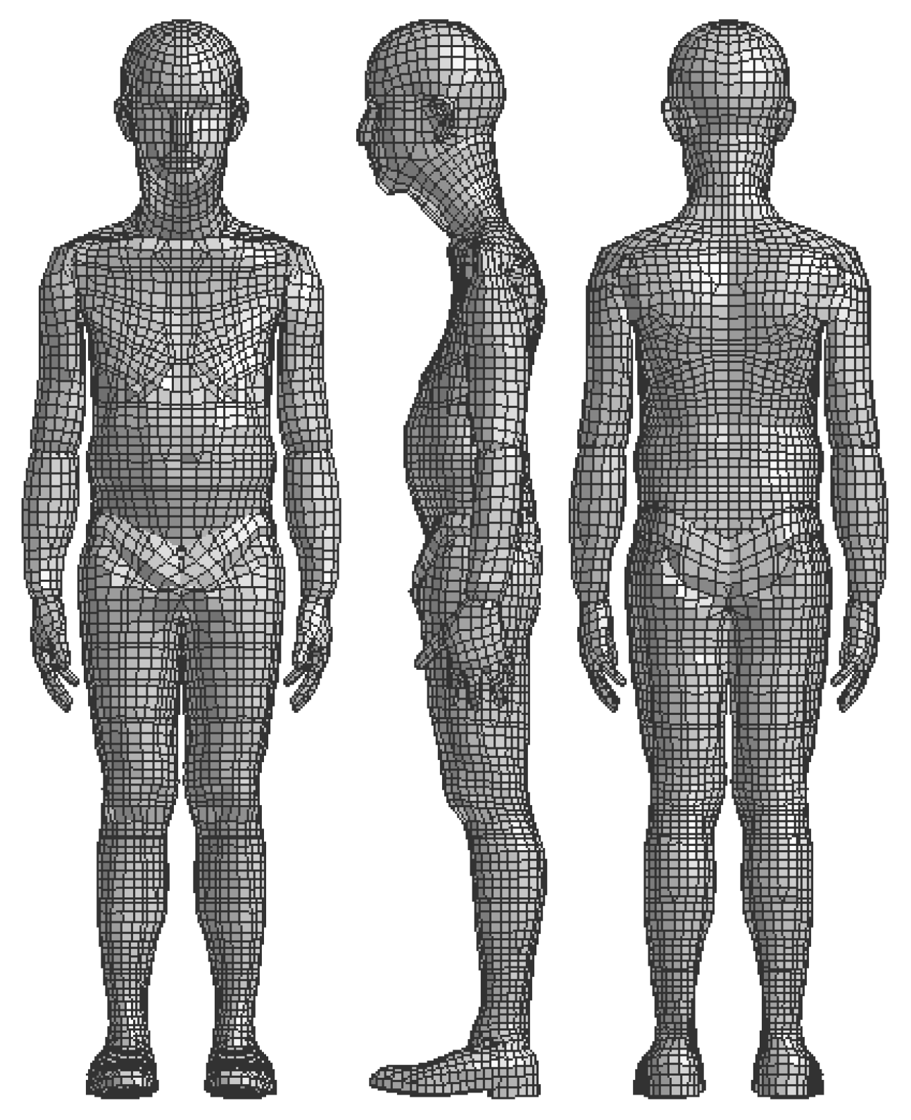
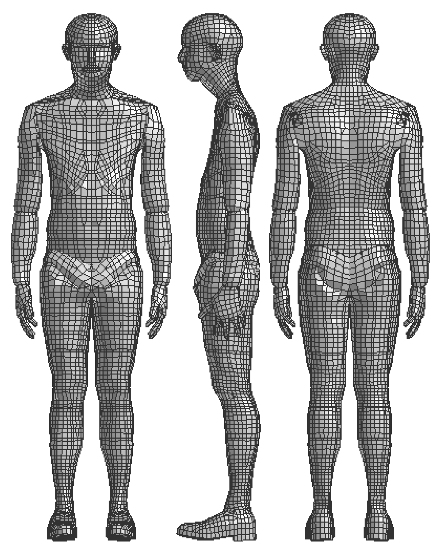
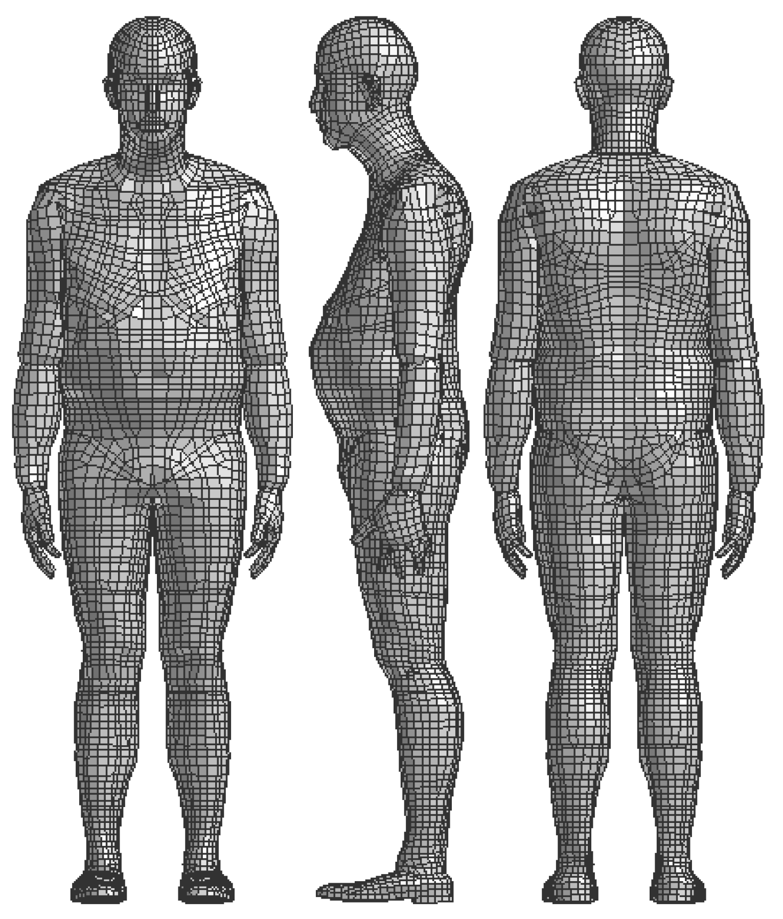
15]. The personalization benefited from the open-tree structure hierarchy, so the base body (to be personalized first) was the abdomen followed by the thorax, neck, and head upwards and the left and right thighs, the left and right calves, and the left and right feet downwards. The thorax was followed by the left and right arms, left and right forearms, and left and right palms. The reference model stood upright so that the local coordinate systems of all segments were aligned to the global coordinate system. The geometry and shape of a particular segment were given by the reference model; see
Figure 2.
Any node
,
(
m being the numbers of nodes on the segment
s) on the scaled model
S is personalized as:
where
is the personalized node on target model
T and
is the transformation matrix for particular segment
s depending on the spatial node position
. Although the personalization in Equation (
2) holds for all segments, the transformation matrix
contains the local scaling (personalization) coefficients to personalize a particular segment
numbered according to
Table 3. For each segment
,
is a diagonal matrix with the space-dependent personalization coefficients in the global coordinate system, so that:
where
for
are the personalization coefficients at location
in the global coordinate system for segment
s. We used polynomials of degree
in the form:
to interpolate the personalization coefficient along each axis
. A lower index
for
was chosen from set
as numbered according to
Table 2. Vector
contains the polynomial coefficients for segment
in direction
. Generally, indication
means the interpolation polynomial of degree
n interpolating the personalization coefficient as the ratios of
anthropometric dimensions (see
Figure 1) as:
where lower indexes
T and
S mean target (personalized) and scaled dimensions, respectively, and
is the dimension number as numbered according to
Table 2 and shown in
Figure 1. For simplification in the further text, we indicate the personalization coefficient
. In particular, for example, 15 means the neck circumference and 17–16 means the calf height (as it must be calculated by subtracting the thigh length from the leg length). For example, polynomial P(23) indicates a constant polynomial calculated as the ratio:
polynomial P(17–16) indicates a constant polynomial calculated as the ratio:
polynomial P(13,14) indicates a linear polynomial interpolating the personalization coefficient between points:
and polynomial P(6,7,3,4,5) indicates a polynomial of degree 4 interpolating the personalization coefficient between points:
The polynomial interpolation might suffer from inaccuracy and unrealistic overshoots in the polynomial shape if we interpolate incomparable values, which is why the scaling was carried out in the first step to approach the target shape, which was refined by personalization.
For each segment, we firstly personalized the height based on the vertical dimensions (1), (8), (9), (10), (11), (16), (17), and (22), as shown in
Figure 1 by means of numbering according to
Table 2. The height of each segment was personalized constantly, meaning that:
is the constant personalization coefficient for the particular segment height.
The frontal (segment depth) and lateral (segment width) personalization depended on the circumference dimension of the particular segment. The circumference dimensions were (2), (3), (4), (5), (12), (13), (14), (15), (18), (19), (20), (21), and (23), as shown in
Figure 1 by means of numbering according to
Table 2. As many segments were described by circumference at the different horizontal location, the polynomials of the degree
interpolated the personalization coefficient along axes
x and
y depending on axis
z, which led to the exact circumferences according to
Figure 1 in the personalized model, so:
where
and
is the polynomial degree. We used the same polynomial degree
for axes
x and
y for segment
s, because the polynomials were formed by the same number of circumference dimensions for each segment.
Figure 1 also defines additional width dimensions, in particular (6) and (10), which were useful as additional measures for personalization. The personalization of each segment is described in detail in the following paragraphs.
2.5.1. Abdomen
The abdomen was the reference segment to be personalized first after the scaling. The reference point was the H-point. According to
Figure 1, the height was personalized by a constant coefficient calculated as the ratio (between the target and scaled models) of the abdominal height (22), from which we subtracted the length from the crotch to the ankle (17) and the ankle height (51). (51) is a new dimension, which is not addressed in the clothing industry, so we took it from the scaled model. As the abdomen and the thorax form a continuous segment, the polynomials interpolating the personalization coefficient in depth and width were formed together along the abdomen and the thoracic height. They were of degree 4 as they addressed 5 circumference dimensions. The depth was personalized along axis
z from the hip circumference at the widest point (5) over the waist circumference at the point of the trousers (4), the waist circumference at the narrowest point (3), and the thoracic circumference at the widest point (7) to the neck circumference (15), where the neck circumference seemed to be a good measure for the upper thoracic depth. The width was personalized along axis
z from the hip circumference at the widest point (5) over the waist circumference at the point of the trousers (4), the waist circumference at the narrowest point (3), and the back width (7) to the shoulder width (6).
2.5.2. Thorax
The thorax follows the abdomen at the joint between vertebrae T12 and L1 [
21], which was also the reference point. As the thorax height was defined by 2 dimensions in the sternum, and on the back, the height was personalized linearly between the front length from the neck to the waist (8) and the back length from the neck to the waist (9), according to
Figure 1. The depth and width were personalized using the same polynomials as for the abdomen.
2.5.3. Neck
The neck follows the thorax at the joint between vertebrae C7 and T1 [
21], which was also the reference point. According to
Figure 1, the height was personalized by a constant coefficient calculated as the ratio of the total body height without shoes (1), from which we subtracted the back length from the neck to the waist (9) and the abdominal height (22). As height 1–9–22 is the total height of the neck and the head, the same personalization coefficient was used for the head height. The depth was personalized by a constant coefficient using the neck circumference (5). The width was personalized along axis
z from the bottom neck using the neck circumference (15) over the neck circumference (15) to the head, where the personalization coefficient held the neck circumference ratio (15). Sixty-two is a new dimension, which is not addressed in the clothing industry, so we took it as the double shoulder length (10) subtracted from the back width (6).
2.5.4. Head
The head follows the neck at the clivus [
21]. As height 1–9–22 is the total height of the neck and the head, the same personalization coefficient was used for the head height. The height personalization used the same personalization coefficient as the neck used. The head size is not typically measured for the means of the clothing industry, so the coefficients were missing. Therefore, the depth and width were personalized by a constant coefficient using the head circumference (23), which was measured.
2.5.5. Arm
The arm follows the thorax in the shoulder joint [
21]. The height (actually the length of the arm) was personalized using a constant coefficient defined by subtracting the shoulder length (10) from the sleeve length from neck to wrist (11). The depth was personalized by a parabolic polynomial based on the arm circumference (12). The polynomial held the arm circumference ratio (12) in the elbow and the thoracic width ratio (6) at its height, which brought a realistic shape to the personalized arm. The width was personalized by a constant coefficient based on the arm circumference (12).
2.5.6. Forearm
The forearm follows the arm at the elbow joint [
21]. The height personalization used the same personalization coefficient as the arm used. The depth and width were personalized using the same linear polynomials interpolating the ratios between the forearm circumference (13) and the wrist circumference (14).
2.5.7. Palm
As the palm is not typically measured in the clothing industry and its small size, mass, and inertial effects do not influence any dynamical action considerably, the palm was not personalized, and only the dimensions arising from of the scaling were taken into account.
2.5.8. Thigh
The thigh follows the abdomen in the hip joint [
21]. According to
Figure 1, the height was personalized by a constant coefficient addressing the ratio of the length from crotch to knee (16). The depth and width were personalized using the same cubic polynomials interpolating the ratios between the hip circumference at the widest point (5), the thigh circumference (18), and the knee circumference (19).
2.5.9. Calf
The calf follows the thigh in the knee joint [
21]. The height was personalized by a constant coefficient defined by subtracting the length from the crotch to the knee (16) from the length from the crotch to the ankle (17). The depth and width were personalized linearly using the same polynomials interpolating the ratios between the calf circumference (20) and the ankle circumference (21).
2.5.10. Foot
The foot follows the calf in the hip ankle joint [
21]. As the foot is not typically measured in the clothing industry and its small size, mass, and inertial effects do not considerably influence any dynamical action, the foot was not personalized, and only the dimensions arising from of the scaling were taken into account.
As the human body is expected to be symmetric, the personalization of the left and right arms, forearms, palms, thighs, calves, and feet was the same.
Table 4 summarizes the personalization of all segments using the polynomial interpolation of the personalization coefficients along the coordinate axes.
As the reference human body model was developed for dynamical analysis, the last step was updating the masses and inertias of the particular segments concerning the shape change, as well as the ranges of the particular joints concerning the age using the same approach as described and published by Hynčík et al. [
7].
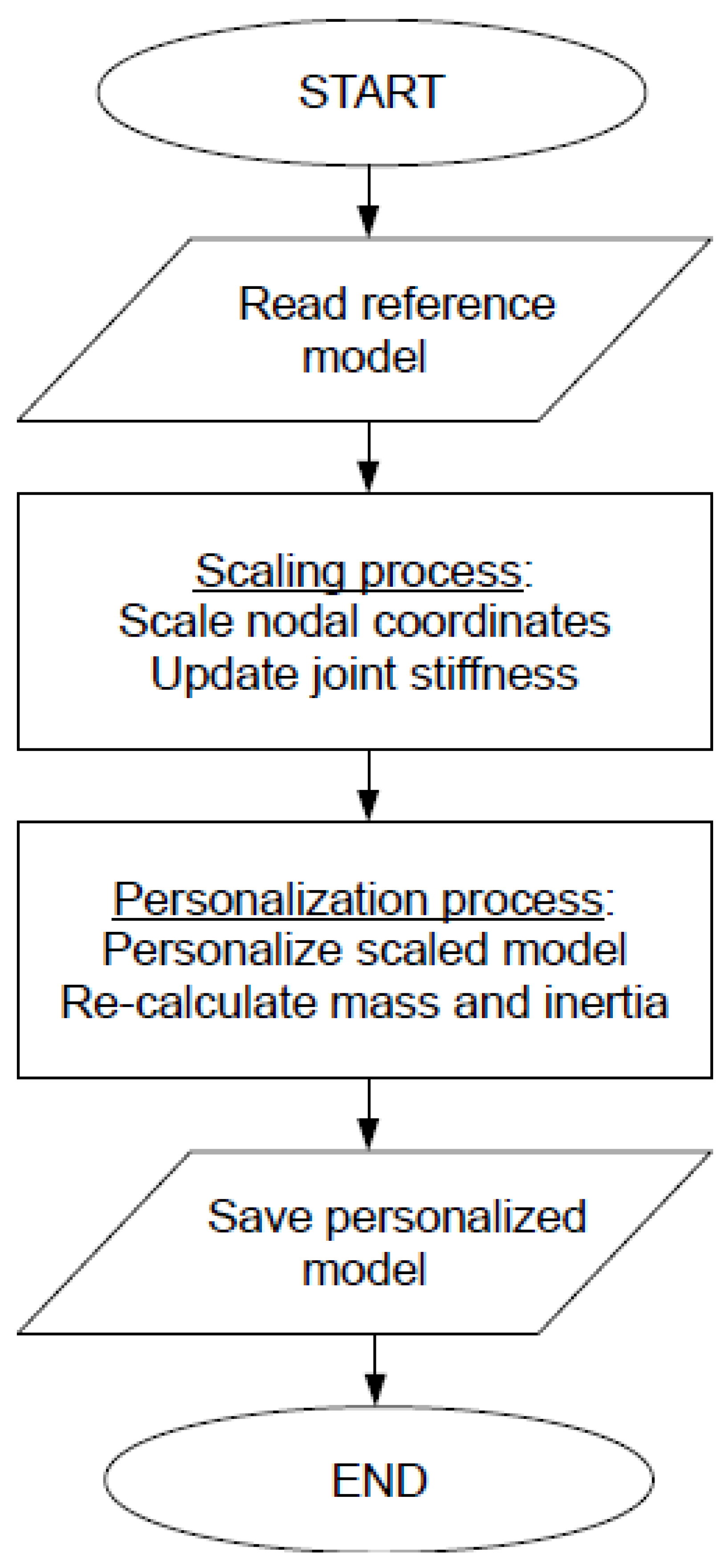
The personalization process was implemented in Python. The Python script first reads the structure of the reference model as the finite element model [
15]. The structure concerns the multibody system, which separates the particular segments and their nodes representing the geometry into rigid bodies. The next step was the scaling of nodal coordinates and updating the stiffness of the joints, which was updated independently using the approach previously developed and published [
7,
25].
After the scaling of each segment, the personalization ran. Then, the segment masses and inertia were recalculated based on the particular segment volume and shape change using the approaches previously developed and published [
7]. After that, the segments were connected back together, as the volume and shape changes affected the location of the joints. Finally, the new model was saved using the updated nodal coordinates, rigid bodies, and joints. The joint stiffness was updated in parallel. The elements defining the body surface were kept as they followed the change of their nodal coordinates. The process flowchart is as follows:
The optimization loop is illustrated in
Appendix A as a flowchart.


 ,
, 


