Analysis of Water Consumption in Fruit and Vegetable Processing Plants with the Use of Artificial Intelligence

Abstract

Fruit and vegetable processing has a significant impact on the environment due to its consumption of a significant amount of water. Water consumption mainly depends on the type of production and the technology used. Water in fruit and vegetable processing plants is used as a raw material, an energy carrier, and in hydro transport, as well as for washing raw materials and maintaining production hygiene. The variety of technological operations carried out in the production process and the seasonality of production make it difficult to objectively assess the use of water in fruit and vegetable processing plants. Few available publications in this field provide numerical values of water unit consumption indices, with none entering into the cause-and-effect relationships of water use in plants in this industry. The aim of this study was to analyze the research to date and to verify the following research hypothesis: the structure of processing and the relationship between the weights of individual products have an impact on water consumption in fruit and vegetable processing plants. For this purpose, neural models of water consumption were developed for the largest agri-food processing plants in Poland that use similar technology. Water consumption was then optimized using genetic algorithms for the processing structure. The results confirmed the hypothesis that production structure has a significant impact on the rationalization of water consumption. The optimization results show that the production of concentrates, juices, and drinks has the greatest impact on water consumption. The lowest water consumption will be achieved when the production of concentrates is at a 2 to 1 ratio to the production of juices and drinks.

1. Introduction

Most of the Polish businesses operating in the fruit and vegetable industry are small and medium enterprises employing less than 250 employees. Large enterprises account for only about 15% of businesses, but they hold a major share of the quantity of fruit and vegetables processed in Poland. Large enterprises produce several types of products, while small enterprises are predominantly oriented towards one product. Typical industry products include fruit juices and drinks, fruit and vegetable concentrates, and frozen fruit and vegetables. In fruit and vegetable industry plants, water is both a raw material and energy carrier; it is used in hydro-transport, for raw material washing, and for the maintenance of production hygiene [1]. The diversity of the technological operations performed in the production process, as well as the seasonality of production, make the objective assessment of water consumption in fruit and vegetable processing plants difficult [2]. The few available publications on this subject specify the numerical values of unit consumption indices without any in-depth analysis of the cause-and-effect relationships in the use of water in the facilities of this industry. Artificial neural networks are used in the study of biosystems in which it is difficult to formally describe the analyzed parameters. In the literature, there are many examples of this type of use of artificial neural networks, for example, to forecast corn and soybean yields [3], the stage of development of sweet pepper fruits [4], fuel consumption in vehicles [5], or river flow [6]. For predicting corn and soybean yields, the authors of [3] proposed a new convolutional neural network model called YieldNet, which utilizes a novel deep learning framework that uses transfer learning between corn and soybean yield predictions by sharing the weights of the backbone feature extractor. Similarly, in [4], an ensemble model of convolutional neural network (CNN) and multilayer perceptron (MLP) models was developed to detect sweet pepper fruits in images and predict their development stages. In the forecasting of fuel consumption in vehicles, the adopted research methodology was based on the use of MLP artificial neural networks and sensitivity analysis. It is very difficult to predict desired water flow using physically based models and conventional regression-based methods due to the nonlinear and fuzzy nature of hydrological activity and the scarcity of relevant data. These traditional methods are incapable of handling the complex non-linearity and non-stationary process of water flow. Thus, the aim of [6] was to develop an intelligent hybrid artificial intelligence model, namely, a genetic-algorithm-based Artificial Neural Network (GA-ANN) for monthly water flow prediction in the Mahanadi river system. All parameters associated with the artificial neural network (ANN) model were simultaneously optimized automatically using the Genetic Algorithm (GA) for the prediction of the water flow. In this study, it was also decided to use artificial neural networks and genetic algorithms to analyze water consumption in fruit and vegetable processing plants.

The objective of this paper was to elaborate on existing research and verify the following research hypothesis: processing structure and the relationship between the weights of specific products have an impact on water consumption in fruit and vegetable processing plants. For this purpose, neural water consumption models were developed from the largest agricultural and food processing plants in Poland that employ similar technology. Subsequently, water consumption was optimized, using genetic algorithms, in relation to processing structure. The analysis of the existing research on water consumption in fruit and vegetable companies and the results of optimization may constitute guidelines for rationalization in water management.

2. The Literature Review

The results of the tests of selected indicators of specific water consumption W_w are given in

Table 1. Water consumption index per product unit in fruit and vegetable industry plants.

Production, Water Intake Directions		Unit water Consumption Indices (m3/mg of Product)		Source
		Index Range *	Numerical Value
Tomato juice thickening in rotary evaporators - AC 100 (35.2 kg/(m2·h)) - AC 200 (40.0 kg/(m2·h)) - PR 16 (31.8 kg/(m2·h))		A	94.5 101.1 85.3	[7]
Fruit washing Vegetable washing Vegetable peeling Blanching Refrigerating		T	1.0–4.0 1.8–2.5 3.0–5.0 0.5–1.0 0.5–1.5	[8]
Marmalades, preserves Fruit juices Retort fruit preserves Retort vegetable preserves Salad preserves		T	6.5 4.5 2.5–4.0 3.5–6.0 3.0	[9,10]
Nectars Liquid fruit Tomato juice Concentrated fruit juices		T	16.0 9.0–11.0 13.0 140.0	[11]
Canned fruit Canned vegetables Frozen vegetables Fruit juices Jams Preserves for children		T	2.5–4 3.5–6 5.0–8.5 6.5 6.0 6.0–9.0	[12]
Frozen fruit		Z	1.3–4.0	[13]
Fruit processing Vegetable processing		Z	2.2–8.2 5.8–20.3	[14]
Fruit and vegetable processing plants	Poland	Z	12.0–32.0 **	[15]
			5.0–61.3	[16,17]
	Finland	Z	1.5–5.0	[18]
	South Africa	Z	0.7–1.9 **	[19]

* A—aggregate index; T—technological index; Z—plant index; ** in relation to 1 mg of raw material.

.

The presented indices are diversified, which results from both the differences in the technical equipment of the plants and the diversity of methods of determination of the said indices [20]. The indices may be data intended for the design of new plants or estimations of the future demand for water. The plant unit water consumption indices W_w contribute the most information. Admittedly, the literature partially specifies the variability ranges of plant unit water consumption indices but does not list many factors that could affect their numerical values. Method basics with this scope can be found in publications [21,22]. Publication [22] presents the general characteristics of sixteen production plants. Daily water consumption in the summer–autumn period ranged from 55.2 to 5431.8 m³. Units of water consumption in the analyzed plants differed more than sevenfold.

The following questions can be posed in this context:

• How can the variability of water consumption by plants in this industry be explained?
• How can the optimum water consumption in a given plant be determined?

In order to respond to the first question, the determining factors and strength of their impact on water consumption A_w and, subsequently, on the values of unit consumption indices W_w, must be determined. The authors of publication [22] presented exemplary groups of factors (independent variables) that affect the consumption of water, covering the scope of the plant index,

Table 2. Factors affecting water consumption in production plants.

Group of Factors	Meaning, Physical Sense	Applied Markings
I	Value generally characterizing the plant	V1,
II	Elements of the structure of installed power of the plants	P1,
III	Structure of daily production	Z1, Z2, Z3
IV	Level of technical and technological equipment and production organization	K2

.

The following formula was adopted to explain the dependence of y on independent variables (being the actual parameters observed in practice or their functions):

y = b₀ + b₁ x₁ + b₂ x₂ +........+ b_k x_k;

(1)

where y is the dependent variable (A_w or W_w) and x represents the independent variables (presented in

Table 3. Factors affecting water consumption variability in the fruit and vegetable industry plants.

Group of Independent Variables	Multiple Regression Equations	R2	Independent Variables
			Determination, Dimension	Numerical Range
I	Aw = −1777.0 + 150. 88 ·$\sqrt{V_1}$	0.395	V1 (m3)	10,008–572,645
II	Aw = 408.4 + 2.30 ·P1	0.543	P1 (kW)	41–1715
III	Aw = 2180.0 − 1420.0/Z1 + 661.6 · logZ2 +140.50 ·$\sqrt{Z_3}$	0.476	Z1 (mg) Z2 (mg) Z3 (mg)	3.8–105.0 64.0–773.0 11.1–191.1
IV	Ww = 1.4 +0.005K2	0.843	K2 (m3/mg)	563–307,692

where A_w is the daily water consumption (m³); K₂ = V₂ Z⁻¹ is the total cubic volume of the plant per 1000 kg (1 mg) of the raw material processed in a day (m³/mg); P₁ is the power of electrical equipment installed in the plant boiler room, pump room, and water treatment station (kW); R² is the correlation coefficient; V₁ is the cubic volume of the production rooms of the plant (m³); V₂ is the total cubic volume of the plant (m³); W_w =A_w Z⁻¹ is the plant unit water consumption index (m³/mg of raw material); Z is the daily raw material processing throughput (mg); Z₁ is the daily production of frozen vegetables (mg); Z₂ is the daily production of fruit concentrates (mg); and Z₃ is the daily production of drinks (mg).

).

Factor groups I–III contributed to the impact on daily water consumption A_w, ranging from 39% to 54%. Admittedly, daily water consumption A_w showed high disproportions among the analyzed plants, but its variability was 54%, attributable to the power of the electrical devices installed in the plant boiler room, pump room, and water treatment station (P₁). The production structure expressed as Z₁ (production of frozen vegetables), Z₂ (production of fruit and vegetable concentrates), and Z₃ (production of drinks) covered by group II contributed about 45% of the impact on the daily water consumption A_w. The application of factor group IV is a source of information on the total impact of technical and technological factors, the degree of automation of the production operations, and organizational–production factors on water consumption. The variability of the unit water consumption W_w was 84.3%, attributable to the impact of factor K₂ (total cubic volume per 1 mg of raw material processed in a day). The application of the obtained equations depends on the ranges of the specific independent variables, the numerical values of which are presented in Table 3.

The reasons for excess water consumption usually include:

• Lack of fully closed circuits of process water (e.g., from washing) and (mainly) cooling water [23];
• Ineffective recovery of the condensate;
• Lack of water consumption optimization in the washing processes (both automatic and manual); the leakage of pipelines, valves, and machinery; and the lack of full supervision over water consumption in specific technological processes.

In the ongoing operation of the production plants, the factor groups I, II, and IV specified in Table 1 have a minor impact on water consumption rationalization. The main impact on rationalization of water consumption is exerted by factor group III. Reduction of unit water consumption must be achieved by the application of the best available techniques in the scope of water management [24]. Rationalization of water consumption in fruit and vegetable industry plants is possible, mostly for entities that carry out monitoring with this scope. The research results presented in Table 3 only partially explain the impact of the processing structure (factor group III) on water consumption. The regression coefficients only determine the degree to which changes of specific parameters Z₁, Z₂, and Z₃ per unit affect the changes in daily water consumption A_w.

It may be added that 270 m³ of wastewater with a highly variable composition is drained daily from an exemplary refrigeration station [19]. On the other hand, a fruit and vegetable processing plant operating year-round produces from 3630 to 4540 m³ of wastewater daily. This information is significant in determining the pollution load and the impact of the fruit and vegetable plants on the environment, taking into account the value of biochemical oxygen demand (BZT₅). Observations in the analyzed plants showed that increasing the use of condensate (water from the concentration of fruit juices) offers substantial water-saving potential. Lipowski [25] presented water consumption reduction options in the production of meat and vegetable preserves from 1.5 to 7.5 (m³/mg). A review of water consumption reduction options in vegetable blanching is presented in [26].

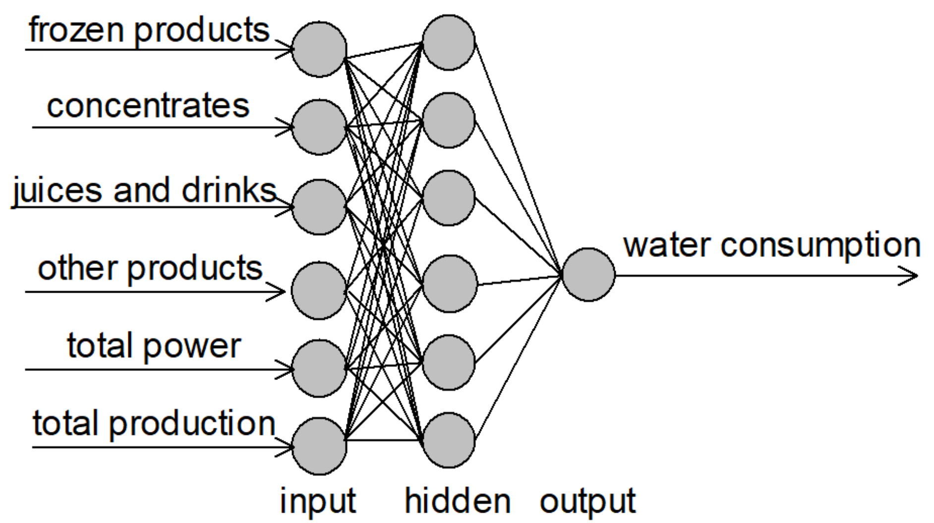
3. Neural Model of Water Consumption

Water consumption tests were carried out in large processing plants in the fruit and vegetable industry that used similar technologies and diversified processing products. For the construction of neural models, 634 data sets of water consumption in fruit and vegetable processing plants were used—all were normalized to obtain values in the range [0,1] by dividing them by maximum values. The purpose of modeling was to prepare the objective function for optimization.

In order to select the optimal structure of the neural network, 35 numerical simulations (

Table 4. Optimization of the neural network architecture.

Simulation No.	Division of Each Sample into Train-Valid-Test Sets	Activation Function in the Hidden Layer	Number of Neurons in the Hidden Layer	Activation Function in the Output Layer	Statistical Performance
					MSE	R-Value	R—Adjusted
1	60-20-20	log-sig	10	log-sig	0.00909	0.92052	0.94955
2	60-20-20	log-sig	14	log-sig	0.01295	0.85946	0.80006
3	60-20-20	log-sig	6	pureline	0.00882	0.90510	0.92124
4	60-20-20	log-sig	10	pureline	0.01115	0.89047	0.93475
5	60-20-20	log-sig	14	pureline	0.00569	0.93186	0.92554
6	60-20-20	tansig	6	pureline	0.01105	0.87170	0.93544
7	60-20-20	tansig	10	pureline	0.01012	0.88376	0.98881
8	60-20-20	tansig	14	pureline	0.00724	0.94758	0.96594
9	60-20-20	tansig	6	log-sig	0.01227	0.85771	0.84561
10	60-20-20	tansig	10	log-sig	0.01046	0.90830	0.83945
11	60-20-20	tansig	14	log-sig	0.01151	0.91263	0.94033
12	70-15-15	log-sig	6	log-sig	0.00656	0.94070	0.88573
13	70-15-15	log-sig	10	log-sig	0.00839	0.90687	0.99758
14	70-15-15	log-sig	14	log-sig	0.01024	0.91473	0.96854
15	70-15-15	log-sig	6	pureline	0.00779	0.88962	0.88017
16	70-15-15	log-sig	10	pureline	0.01127	0.90074	0.99739
17	70-15-15	log-sig	14	pureline	0.01032	0.90545	0.89289
18	70-15-15	tansig	6	pureline	0.00977	0.89027	0.97076
19	70-15-15	tansig	10	pureline	0.00856	0.91127	0.71730
20	70-15-15	tansig	14	pureline	0.01171	0.85632	0.83473
21	70-15-15	tansig	6	log-sig	0.01130	0.89255	0.97375
22	70-15-15	tansig	10	log-sig	0.00654	0.92229	0.83440
23	70-15-15	tansig	14	log-sig	0.01516	0.80701	0.99803
24	80-10-10	log-sig	6	log-sig	0.00411	0.95967	0.94904
25	80-10-10	log-sig	10	log-sig	0.00788	0.92798	0.90828
26	80-10-10	log-sig	14	log-sig	0.01172	0.87754	0.92124
27	80-10-10	log-sig	6	pureline	0.02016	0.82914	0.92241
28	80-10-10	log-sig	10	pureline	0.00986	0.91291	0.91322
29	80-10-10	log-sig	14	pureline	0.01231	0.88508	0.99082
30	80-10-10	tansig	6	pureline	0.00637	0.9521	0.94621
31	80-10-10	tansig	10	pureline	0.01315	0.88489	0.9999
32	80-10-10	tansig	14	pureline	0.01241	0.85400	0.85677
33	80-10-10	tansig	6	log-sig	0.00761	0.90785	0.96694
34	80-10-10	tansig	10	log-sig	0.00901	0.94803	0.95231
35	80-10-10	tansig	14	log-sig	0.00782	0.92660	0.96451

) were carried out in the MATLAB program [27]. The variable parameters were divided into the training, validation, and test sets (column 2); activation functions in the hidden and output layer (columns 3 and 5); and the number of neurons in the hidden layer (column 4). The assessment criteria for the conducted numerical simulations were the smallest root mean square error (MSE), correlation coefficient R for the validation set, and R—adjusted value (columns 6, 7, and 8). All tested models were implemented in the MATLAB neural network and trained according to Levenberg–Marquardt learning algorithm.

The conducted simulations show that neural network no. 24 demonstrated the smallest root mean square error (MSE = 0.00411) and the highest correlation coefficient (R = 0.95967) (see Table 4). In this case, the samples were randomly divided into the following sets: for training, 80 % of samples; for validation, 10% of samples; and for testing, 10% of samples. Figure 1 shows ANN regression plots between outputs and target samples. The R values in each case are greater than 91%. Therefore, the fit is reasonably good for all data sets. Additionally, R for the water consumption was estimated as 0.90774 for training, 0.88705 for testing, and 0.95967 for validation data sets.

Figure 2 presents the optimal structure of the neural network. The neural network consisted of three layers (input, hidden, output). The input layer contained six decision variables: frozen products (x₁), concentrates (x₂), juices and drinks (x₃), other products (x₄), total power (x₅), and total production (x₆). Water consumption (y) was in the output layer. As shown in Figure 2, 6 neurons were located in the hidden layer. The activation function, both in the hidden and output layers, was the “log-sigmoid” function. Therefore, the topology with six inputs, six neurons with one hidden layer, and one output (6-6-1) was applied for predicting water consumption.

For the created model, a sensitivity analysis was performed, obtaining the importance of individual input variables. It is assumed that a given input variable is more important the greater the increase in the error value caused by its removal (

Table 5. Neural network (MLP 6-6-1) sensitivity analysis.

Neural Network	Sensitivity Analysis
	X6	X5	X3	X2	X1	X4
MLP 6-6-1	3.19527	2.136989	1.804672	1.763347	1.628497	1.494883

).

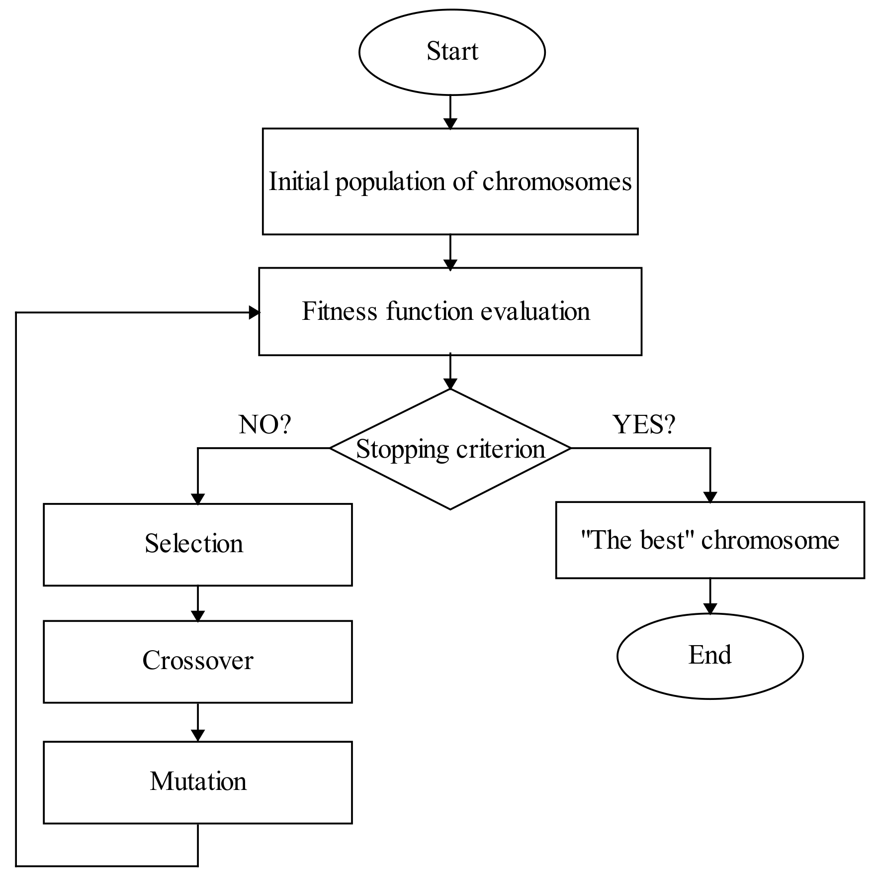
4. Optimizing Water Consumption

Based on the neural modeling results, the objective function was formulated Dependences (2–8):

$$min y=\frac{1}{1+e^{-\left(5.9157·\mathrm{F}1-6.3083·\mathrm{F}2+4.5594·\mathrm{F}3+4.0588·\mathrm{F}4-4.2846·\mathrm{F}5-6.8515·\mathrm{F}6-3.2504\right)}}$$

(2)

$$F1=\frac{1}{1+e^{-\left(2.2541·x_1-3.2955·x_2-4.1841·x_3+7.6881·x_4-0.5265·x_5+0.8106·x_6-3.0717\right)}}$$

(3)

$$F2=\frac{1}{1+e^{-\left(1.8281·x_1+3.2851·x_2-0.4512·x_3-9.7172·x_4-5.3785·x_5-2.9250·x_6+2.2943\right)}}$$

(4)

$$F3=\frac{1}{1+e^{-\left(3.7724·x_1-13.1648·x_2+7.1149·x_3-2.7830·x_4-3.3761·x_5-8.6733·x_6+6.7341\right)}}$$

(5)

$$F4=\frac{1}{1+e^{-\left(1.9877·x_1+1.3262·x_2-8.1159·x_3-2.2637·x_4-1.9505·x_5-0.5714·x_6+3.2822\right)}}$$

(6)

$$F5=\frac{1}{1+e^{-\left(5.6527·x_1-10.8427·x_2-8.9566·x_3+7.1270·x_4+4.1863·x_5-1.9187·x_6-2.5376\right)}}$$

(7)

$$F6=\frac{1}{1+e^{-\left(-2.8516·x_1-7.7136·x_2-0.6023·x_3+4.6774·x_4+0.1839·x_5-0.8577·x_6-0.5875\right)}}$$

(8)

where the numeric constants (weights and biases) from Equations (1)–(6) were derived from the neural network structure. The input data x₁, x₂, x₃, x₄, x₅, and x₆ were normalized, dividing them by the respective numbers 282, 773, 312, 304, 14054, and 778. The output data y were multiplied by 7316.

The purpose of optimization was the minimization of water consumption y Equations (2)–(8) for the decision variables x₁–x₆ in the scope of their upper and lower limits. The limitations were Dependences (9–15):

0.38 < x₁ < 282,

(9)

0.585 < x₂ < 773,

(10)

0.675 < x₃ < 312,

(11)

0.44 < x₄ < 304,

(12)

946 < x₅ < 14054,

(13)

1.63 < x₆ < 778,

(14)

x₁ + x₂ + x₃ + x₄ = x₆

(15)

Genetic algorithms are an optimization method that relies on the natural processes of evolution. The main genetic parameters are crossover and mutation. These parameters determine the selection of the best individuals for the next generation (iteration). The main steps of the genetic algorithm are presented in Figure 3. These are selection, calculation of the objective function, and application of genetic operators (crossover and mutation). After each iteration, all steps are repeated until the best solution (chromosome) is obtained.

Optimization was carried out using the genetic algorithm in the “Optimization” tool provided by the MATLAB software.

Table 6. Genetic algorithm parameters.

Population Size	Crossover Probability	Mutation Probability	Number of Generations
$N_{size}$	$p_k$	$p_m$	$N_{gen}$
80	0.8	0.01	3000

presents the genetic algorithm parameters adopted for optimization. The population size, crossover probability, mutation probability, and number of generations were determined by trial and error and on the basis of literature data [28].

Figure 4 presents the results of water consumption optimization by means of the genetic algorithm. The upper chart (Figure 4) presents the course of the objective function in the specific generations. The chart shows a sudden drop in the objective function after 400 generations. The function value declined from 6000 to 10. Further operation of the genetic algorithm yielded the lowest value of the objective function, i.e., y = 3.86 after 300 generations. Further operation of the GA did not result in the function’s improvement. The chart below (Figure 4) presents the results of decision variables x_{1 -} x₆ after the genetic algorithm was stopped after 540 generations.

The objective function assumes the lowest value for the decision variables presented in

Table 7. Results of optimization by means of the genetic algorithm.

Frozen Products (mg/day)	Concentrates (mg/day)	Juices and Drinks (mg/day)	Other Products (mg/day)	Total Power (kW)	Total Production (mg/day)
$x_1$	$x_2$	$x_3$	$x_4$	$x_5$	$x_6$
35.06	505.05	237.68	0.44	946	778.24

.

The lowest water consumption of 3.86 m³ a day was obtained at the lower range of the employed production capacity, 946 kW, for which the production of frozen products, concentrates, juices and drinks, and other products was 35, 505, 238, and 0.44 mg/day, respectively. Assuming that the production of frozen products x₁ and other production x₄ is significantly lower, the lowest water consumption can be achieved with a 2 to 1 ratio of concentrate production to juice and drink production.

5. Conclusions

As demonstrated in the analysis of the current state of knowledge, fruit and vegetable processing has a significant impact on the environment due to its consumption of a substantial quantity of water, which must be reduced by means of technological improvement in the scope of water consumption rationalization [29,30]. Water consumption reduction methods include obliging suppliers to supply the raw material in an already treated form, as well as options in the scope of water recovery, e.g., returning transport water back to the circuit. The presented formulas also enable the analysis of the variability of water consumption, taking into consideration significant technical, technological, and other factors, and enable the analysis of the impact of fruit and vegetable processing plants on the natural environment [31]. The presented results may also be useful in environmental reviews. The literature data [32,33,34,35,36] show that comprehensive actions in the scope of water consumption rationalization may result in the reduction of water consumption by up to 50–70%. Rationalization of water consumption in fruit and vegetable processing plants is possible only for entities that carry out monitoring within this scope.

Studies with the use of artificial intelligence, carried out on 634 real data sets, confirmed the hypothesis that the structure of processing is an important factor in rationalizing water consumption. The proposed method enables optimization of water consumption with regard to the type and structure of fruit and vegetable processing. As indicated by the optimization results, for the analyzed fruit and vegetable processing technology, the lowest water consumption will be achieved when the production of concentrates is at a ratio of 2 to 1 to the production of juices and beverages.

References

1. Selma, M.V.; Allende, A.; Lopez-Galvez, F.; Conesa, M.A.; Gil, M.I. Disinfection potential of ozone, ultraviolet-C and their combination in wash water for the fresh-cut vegetable industry. Food Microbiol. 2008, 25, 809–814. [Google Scholar] [CrossRef]
2. Gil, M.I.; Selma, M.V.; López-Gálvez, F.; Allende, A. Fresh-cut product sanitation and wash water disinfection: Problems and solutions. Int. J. Food Microbiol. 2009, 134, 37–45. [Google Scholar] [CrossRef] [PubMed]
3. Khaki, S.; Pham, H.; Wang, L. Simultaneous Corn and Soybean Yield Prediction from Remote Sensing Data Using Deep Transfer Learning. Sci. Rep. 2021, 11, 11132. [Google Scholar] [CrossRef]
4. Moon, T.; Park, J.; Son, J.E. Prediction of the Fruit Development Stage of Sweet Pepper (Capsicum Annum Var. Annuum) by an Ensemble Model of Convolutional and Multilayer Perceptron. Biosyst. Eng. 2021, 210, 171–180. [Google Scholar] [CrossRef]
5. Ziółkowski, J.; Oszczypała, M.; Małachowski, J.; Szkutnik-Rogoż, J. Use of Artificial Neural Networks to Predict Fuel Con-sumption on the Basis of Technical Parameters of Vehicles. Energies 2021, 14, 2639. [Google Scholar] [CrossRef]
6. Yadav, A.; Prasad, B.B.V.S.V.; Mojjada, R.K.; Kothamasu, K.K.; Joshi, D. Application of Artificial Neural Network and Ge-netic Algorithm Based Artificial Neural Network Models for River Flow Prediction. Revue d’Intelligence Artif. 2020, 34, 745–751. [Google Scholar] [CrossRef]
7. Lewicki, P.P.; Skierkowski, K.; Wrzeszcz, S. Przemysł Fermentacyjny i Owocowo-Warzywny; Wydawnictwo Czasopism i Ksiazek Technicznych SIGMA-NOT Sp. z o.o: Warszawa, Poland, 1981; pp. 40–42. [Google Scholar]
8. Lipińska-Łuczyn, E. Best Available Techniques (BAT)-Guidelines for the Food Industry: Fruit and Vegetable; Ministry of the Environment: Warszawa, Poland, 2005; pp. 24–27.
9. Henkel, M.; Richter, M. Situation und Aufgaben der Betriebswirtschaft in der obst- und gemüseverarbeitenden Industrie. Wasserwirtsch. -Wassertech. 1981, 10, 358–359. [Google Scholar]
10. Rüffer, H.; Rosenwinkel, K.H. Treatment of Industrial Wastewater; Oficyna Wydawnicza Projprzem-EKO: Bydgoszcz, Poland, 1998; pp. 81–98. [Google Scholar]
11. Neryng, A.; Wojdalski, J.; Budny, J.; Krasowski, E. Energy and Water in the Agri-Food Industry; WNT: Warszawa, Poland, 1990; pp. 280–281. [Google Scholar]
12. Masanet, E.; Woorrell, E.; Graus, W.; Galitsky, C. Energy Efficiency Improvement and Cost Saving Opportunities for the Fruit and Vegetable Processing Industry; University of California: Berkeley, CA, USA, 2007; pp. 115–126. [Google Scholar]
13. Kwas, A. Determinants of the Consumption of Energy Carriers in a Fruit Processing Plant. Master’s Thesis, Wydział Inżynierii Produkcji, SGGW, Warszawa, Poland, 2018. [Google Scholar]
14. Grzybek, A. The impact of selected technologies on the environment and energy consumption in fruit and vegetable processing. Rozprawy habilitacyjne nr 12. Inżynieria Rolnicza 2003, 2. [Google Scholar]
15. WS Atkins International. Environmental Protection in the Agri-Food Industry. Environmental Standards; FAPA: Warszawa, Poland, 1998; Volume 57, p. 88. [Google Scholar]
16. Strzelczyk, M.; Steinhoff-Wrześniewska, A.; Rajmund, A. Indicators of water consumption and the quantity of wastewater formed in selected branches of food industry. Polish J. Chem. Technol. 2010, 12, 6–10. [Google Scholar] [CrossRef] [Green Version]
17. Steinhoff-Wrześniewska, A.; Rajmund, A.; Godzwon, J. Water consumption in selected branches of food industry. Inżynieria Ekologiczna 2013, 32, 164–171. [Google Scholar] [CrossRef] [Green Version]
18. Lehto, M.; Sipilä, I.; Alakukku, L.; Kymäläinen, H.R. Water consumption and wastewaters in fresh-cut vegetable production. Agric. Food Sci. 2014, 23, 245–256. [Google Scholar] [CrossRef]
19. Kubicki, M. Environmental Protection in the Fruit and Vegetable Industry; FAPA: Warszawa, Poland, 1998; pp. 34–35, 38–43. [Google Scholar]
20. Evrard, D.; Villot, J.; Armiyaou, C.; Gaucher, R.; Bouhrizi, S.; Laforest, V. Best Available Techniques: An integrated method for multicriteria assessment of reference installations. J. Clean. Prod. 2018, 176, 1034–1044. [Google Scholar] [CrossRef]
21. Wojdalski, J.; Dróżdż, B. Basics of analysis of energy consumption in production of agricultural and food industry plants. MOTROL Motoryzacja i Energetyka Rolnictwa 2006, 8A, 294–304. [Google Scholar]
22. Wojdalski, J.; Dróżdż, B.; Lubach, M. Factors influencing water consumption in fruit and vegetable processing plants. Postępy Techniki Przetwórstwa Spożywczego 2005, 1, 39–43. [Google Scholar]
23. Montgomery, J.M. Water Recycling in the Fruit and Vegetable Processing Industry; Office of Water Recycling, California State Water Resources Control Board: Sacramento, CA, USA, 1981. [Google Scholar]
24. Derden, A.; Vercaemst, P.; Dijkmans, R. Best available techniques (BAT) for the fruit and vegetable processing industry. Resour. Conserv. Recycl. 2002, 34, 261–271. [Google Scholar] [CrossRef]
25. Lipowski, J. Possibilities of reducing water consumption during the thermal preservation of canned goods. In Proceedings of the Seminar in the Series “Relationships between Science and Practice”. POLEKO’96, Poznań, Poland; 1996; pp. 117–124. [Google Scholar]
26. Miłek, B.; Stelmach, Z.; Stankiewicz, K. Technical possibilities of using waste heat and reducing water consumption in selected technological processes of the fruit and vegetable industry. Przemysł Ferment. Owocowo-Warzywny 1991, 3, 13–14. [Google Scholar]
27. MathWorks-Matlab. Available online: www.mathworks.com (accessed on 21 October 2021).
28. Winiczenko, R.; Kaleta, A.; Górnicki, K. Application of a MOGA Algorithm and ANN in the Optimization of Apple Drying and Rehydration. Processes 2021, 9, 1415. [Google Scholar] [CrossRef]
29. Hickey, M.; Hoogers, R.; Singh, R.; Christen, E.; Henderson, C.; Ashcroft, B.; Hoffmann, H. Maximising Returns from Water in the Australian Vegetable Industry: National Report; NSW Department of Primary Industries: Orange, NSW, Australia, 2006. [Google Scholar]
30. Kumar, R.S.; Manimegalai, G. Fruit and Vegetable Processing Industries and Environment. Industrial Pollution & Management; Kumar, A., Ed.; APH Publishing Corporation: New Delhi, India, 2004; pp. 97–117. [Google Scholar]
31. Asgharnejad, H.; Khorshidi Nazloo, E.; Madani Larijani, M.; Hajinajaf, N.; Rashidi, H. Comprehensive review of water management and wastewater treatment in food processing industries in the framework of water-food-environment nexus. Compr. Rev. Food Sci. Food Saf. 2021, 20, 4779–4815. [Google Scholar] [CrossRef]
32. Almató, M.; Sanmartí, E.; Espun, A.; Puigjaner, L. Rationalizing the water use in the batch process industry. Comput. Chem. Eng. 1997, 21, S971–S976. [Google Scholar] [CrossRef]
33. Carrasquer, B.; Uche, J.; Martínez-Gracia, A. A new indicator to estimate the efficiency of water and energy use in agro-industries. J. Clean. Prod. 2017, 143, 462–473. [Google Scholar] [CrossRef]
34. Mundi, G.S.; Zytner, R.G.; Warriner, K.; Gharabaghi, B. Predicting fruit and vegetable processing wash-water quality. Water Sci. Technol. 2018, 2017, 256–269. [Google Scholar] [CrossRef] [PubMed]
35. Valta, K.; Kosanovič, T.; Malamis, D.; Moustakas, K.; Loizidou, M. Overview of water usage and wastewater management in the food and beverage industry. Desalination Water Treat. 2015, 53, 3335–3347. [Google Scholar] [CrossRef]
36. Volschenk, P.J. Investigating Water and Wastewater Management in the South African Fruit and Vegetable Processing Industry. Master’s Thesis, Stellenbosch University, Stellenbosch, South Africa, 2020. Available online: https://scholar.sun.ac.za (accessed on 21 October 2021).
Figure 1. Correlation coefficients R for the specific sets.
Applsci 11 10167 g001
Figure 2. Schematic neural network architecture.
Applsci 11 10167 g002
Figure 3. Basic steps of the genetic algorithm.
Applsci 11 10167 g003
Figure 4. Results of optimization by means of the genetic algorithm.
Applsci 11 10167 g004