Deep Convolutional Neural Network with KNN Regression for Automatic Image Annotation

Abstract

Automatic image annotation is an active field of research in which a set of annotations are automatically assigned to images based on their content. In literature, some works opted for handcrafted features and manual approaches of linking concepts to images, whereas some others involved convolutional neural networks (CNNs) as black boxes to solve the problem without external interference. In this work, we introduce a hybrid approach that combines the advantages of both CNN and the conventional concept-to-image assignment approaches. J-image segmentation (JSEG) is firstly used to segment the image into a set of homogeneous regions, then a CNN is employed to produce a rich feature descriptor per area, and then, vector of locally aggregated descriptors (VLAD) is applied to the extracted features to generate compact and unified descriptors. Thereafter, the not too deep clustering (N2D clustering) algorithm is performed to define local manifolds constituting the feature space, and finally, the semantic relatedness is calculated for both image–concept and concept–concept using KNN regression to better grasp the meaning of concepts and how they relate. Through a comprehensive experimental evaluation, our method has indicated a superiority over a wide range of recent related works by yielding F1 scores of 58.89% and 80.24% with the datasets Corel 5k and MSRC v2, respectively. Additionally, it demonstrated a relatively high capacity of learning more concepts with higher accuracy, which results in N+ of 212 and 22 with the datasets Corel 5k and MSRC v2, respectively.

1. Introduction

With technological advancement, it is becoming increasingly simple for people to capture photographs at various locations and activities. There are thousands, if not millions, of personal photographs that are frequently stored without any form of significant labeling. As a result, finding desired photographs has become a tedious and time-consuming task.

Image labeling procedure (image annotation) entails giving to a picture one or more labels (tags) that describe its content. This procedure may be used for a variety of tasks, including automatic photo labeling on social media [1], automatic photo description for visually impaired persons [2], and automatic text production from photographs [3]. Since it takes a lot of time and effort, manual image labeling (tagging) is inconvenient for small collections and impossible for huge collections. To address these issues, automatic image annotation (AIA) was developed, and it has since become a vibrant and essential academic topic. AIA models concepts using preannotated photo collections that are already accessible. Thereafter, this learned model will be applied to labeling unidentified images or completing partial labeled ones.

In the literature, several AIA annotation techniques have been proposed, which may be divided into visual-based and semantic-based techniques. Visual-based approaches are mostly used to investigate the link between visual characteristics and textual labels. In addition to feature–concept relationships, semantic approaches also consider the relations between the concepts themselves (concept–concept). The majority of AIA approaches focus on the overall image’s semantic [4,5,6,7,8,9,10,11,12], ignoring the syntax and regional connotations. Because the traits and indicators of various regions are not taken into consideration, such holistic methods cannot discover all important concepts that may be represented within the image. Other region-based methods [13,14,15,16,17,18,19], on the other hand, have emphasized establishing a one-to-one correlation between concept and region (i.e., each region represents one concept). Such a region-level semantic is more beneficial for figuring out the connections between semantic ideas and visual objects in images. Another interesting classification approach of AIA methods is the one proposed by Chen et al. [20], in which the methods are divided into three categories, namely: KNN-based, regression-based, and semantic-hierarchy-based [21,22].

In this paper, we propose a regression-region-based method for AIA. The main objective is to assign, for a given image, a set of labels that each represent one region (object) within the image. KNN regression has been employed to enhance both the representation of regions in the input feature space and the propagation of labels in the output semantic space. Extensive experiments have been carried out to evaluate the performance of the proposed method against other related works.

The remainder of this paper is structured as follows: Section 2 categorizes and presents works that tackle the issue of automatic image annotation. Section 3 introduces our proposal and the rationale behind each of its phases. Section 4 is dedicated to comprehensively evaluating the proposed method and comparing it to other works of AIA. Finally, we draw some conclusions.

2. Related Work

Automatic image annotation (AIA) methods can roughly be categorized into two categories, global- and local-based methods. Global-based AIA methods, such as [8,10,11,23], are not able to correctly assign important semantic concepts, since the properties and semantics of distinct regions are not often taken into account. As a result, local-based techniques have emerged to overcome this challenge by attempting to capture semantics at the region level rather than holistically. In this section, we review works that attempt to solve the problem of AIA at the region level.

Carneiro et al. [24] used a hierarchical model based on Gaussian mixtures to link low-level visual characteristics and then estimated the shared density of visual characteristics on the regions with semantic notions. Strict semantic constraints were imposed on training data to ensure that each keyword is considered as a category. As a result, areas with similar semantic content are divided into groups based on their content similarity. Blei et al. [25] proposed three hierarchical probabilistic mixture models, culminating in the Corr-LDA model, for image annotation in which the joint probabilities between words and regions are estimated. Later on, the Corr-LDA model was improved in [26] by the addition of a class variable above the mixing proportion parameter of the former model. In the improved model, the general scene is classified, each item is recognized and segmented, and the image is marked with a label list.

Another approach to tackling the issue of AIA is by considering the region–concept or concept–concept co-occurrence. Brown et al. [27] first uniformly divide the image into NxM regular grid and then perform vector quantization of the subimages. This leads to results showing that each subimage may be associated with a collection of labels picked from words allocated to the entire image. One major drawback of this model is the need for a large number of training samples to estimate the appropriate likelihood. It also tends to assign repeated words to the same subimage. Inspired by concept–image co-occurrence matrix and machine translation models, the cross-media relevance model [28] emerged and demonstrated the efficiency of learning the codistribution of blobs and keywords. Blobs, in this context, are a result of clustering image features extracted from regions after using some typical segmentation algorithm. Instead of modeling blob-keyword via simple correlation, authors in [29] modeled word probabilities using a multiple Bernoulli model and image feature probabilities using a nonparametric kernel density. In [30], authors proposed a label co-occurrence learning framework based on graph convolution networks (GCNs) to directly examine the dependencies between pathologies for the multilabel chest X-ray. The aforementioned works require large numbers of training samples and have limited generalization ability to new categories. Mori et al. [31] introduced a multilabel few-shot model for general image recognition. It first correlates different labels, based on statistical label co-occurrences, using a structured knowledge graph. The graph is then exploited via network propagation, enabling the learning of contextualized image feature representations. Duygulu et al. [32] regarded the problem of AIA as analogous to machine translation in which one representation form (i.e., region) is desired to be translated to another (i.e., word). By opting for such a model, the correspondence region–label can easily be modeled via a conventional EM algorithm. Thereafter, the authors presented two classes of models for the joint distribution of text–blob and showed how they are applied image annotation [33]

Some other attempts for AIA have been accomplished using machine learning techniques. In [13], images are segmented into regions from which the visual features are extracted and then used to train a new asymmetrical support vector machine-based MIL algorithm (ASVM-MIL). SVM was chosen because of its excellent capacity to learn and distinguish positive from negative examples. After training the SVM and adjusting its margin constraints, several positive bags were obtained and updated to ensure that all positive bags follow the MIL setting. This model attempts to reduce false positives by directly altering SVM’s margin constraints. In [34], images were firstly segmented into regions (i.e., blobs) using maximum variance intraclustering. The correlation between image areas and annotations was learned using a multilabel semantic learning model based on the Bayes classifier which was then applied to predict labels for nonannotated images.

In [18], region-based bag-of-words (RBoW) was used for sparse feature aggregation, and the resulting descriptor was then fed to second-order conditional random fields (CRFs) to enhance the accuracy of AIA. In [16], a new framework was proposed using techniques of semantic analysis, segmentation, and discriminant classification. Images were segmented into regions using an improved JSEG algorithm after which the content of these regions was represented through an extended BoW model. Thereafter, multiclass maximal figure-of-merit (MC-MFoM) was used to build the concept models for image region annotation. This discriminative model was chosen above others (such as SVM and CRF) because it is more resilient, especially when learning sparse data. The authors in [35] attempted to perform scene segmentation using 3D information extracted from the scene, which decomposes a scene into semantically meaningful regions. This method exploits both label-region and region-region semantics.

3. Our Proposal

Conventional AIA algorithms consider the image as holistic by analyzing images globally rather than dealing with each present object. In real cases, however, few concepts may describe the image holistically, such as ‘joy’ or ‘wild’, but most concepts concern some specific regions (areas) of the image, such as ‘football’, ‘human’, or ‘cloud’. As a result, for an AIA system to produce good annotation results, it must account for visual distinctions across regions as well as semantic interconnections between labels. Given that a concept–region co-occurrence matrix is derived from an annotated training image subset, our proposed solution investigates the similarity among characteristics of a candidate region and the training subset using this concept–region co-occurrence matrix. By doing so, we ensure that visual correlations among areas are taken into consideration. Thereafter, we employ a k-nearest neighbors regression (KNN-r) algorithm to annotate new regions. Figure 1 depicts a general scheme of the proposed approach.

As the scheme in Figure 1 shows, our model takes a set D of images D = {I₁, …, I_N}, some of which are labeled (for training) and the rest of which are not. It should be mentioned that each training image I_n is labeled with I_cn concepts: I_cn ∈ C/C = {C₁, …, C_M}. All images are passed through a preprocessing step in which they are segmented, using JSEG algorithm, into visually homogeneous regions. An aggregation approach is subsequently used to decrease the large number of areas by codifying comparable areas into blobs (codebook), with each blob corresponding to one label. Using the generated codebook and the annotation from the training subset, our model generates a co-occurrence matrix that codifies the appearance frequency of each blob–concept. Finally, we engage KNN regression to predict annotations corresponding to blobs extracted from unannotated images. Each of these steps will be further discussed hereafter.

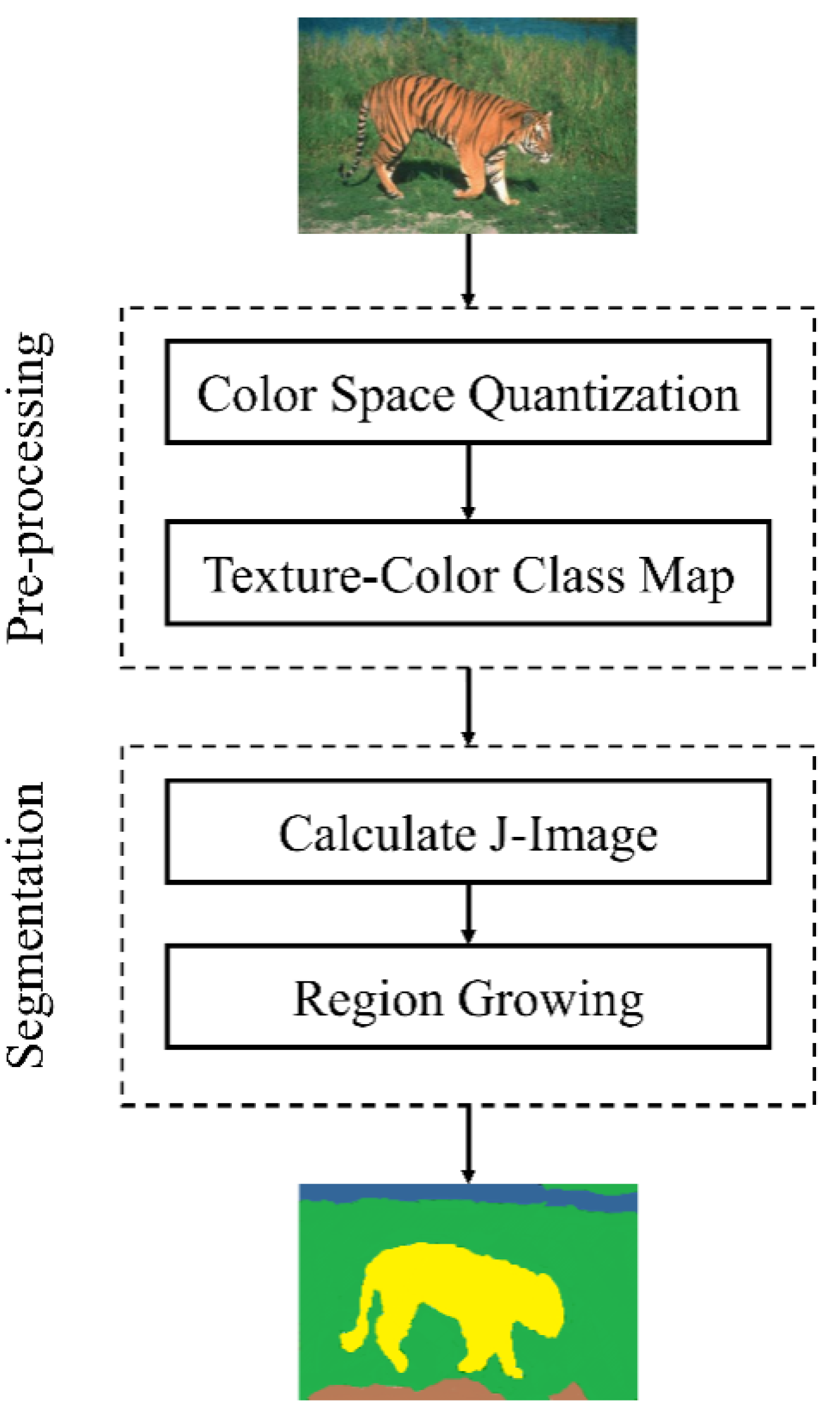
3.1. Image Segmentation Using JSEG Algorithm

According to [36], the best way to recognize objects from an image is to segment them and then extract features from those segmented regions. However, object segmentation, both using supervised and unsupervised approaches, is itself a complex task. Despite the difficulty of achieving precise and accurate semantic segmentation, it has been proven on many occasions that segmented areas hold valuable annotation cues regardless of the quality of segmentation [16,34].

JSEG is a powerful unsupervised segmentation algorithm for color images that proved its effectiveness and robustness in a variety of applications [37,38]. JSEG has recently witnessed various improvements to improve its performances, such as in the problem of oversegmentation [16,39]. In our study, the JSEG proposed in [18] has been employed to segment the image into a set of semantic regions, as illustrated in Figure 2.

3.2. Region Representation

In region-based techniques, the visual characteristics of the image, such as color, texture, and form, are typically extracted from each region. Using local features instead of global ones has been proven to be more effective in image annotation tasks. Nevertheless, appropriate features must be selected to represent the essential substance of the image. For the task of image representation, deep CNNs have recently been shown to outperform, by a significant margin, state-of-the-art solutions that use traditional hand-crafted features. In our study, the learning transfer of off-the-shelf features extracted from a pretrained CNN model has been used to represent the content of each image region. Learning transfer has shown high efficiency in extracting visual features and demonstrated that features with sufficient representative strength can be extracted from the last layers [40,41]. We have opted for a pretrained model for two reasons: the first one is that we do not have a sufficient amount of data or the necessary resources to train a new CNN model; the second reason is to speed up the training process of our model. MobileNet [42] model, shown in Figure 3, has been adopted in the present work since it has proved high performance (both accuracy and rapidness) in many learning transfer-based methods.

3.3. Feature Aggregation

The JSEG algorithm does not necessarily generate an equal number of regions per image. Thus, extracting features from each region usually results in image descriptors with different sizes. To normalize the sizes of image descriptors, an aggregation method is generally utilized to produce a codebook that is used later on to codify the descriptors into equal size descriptors [43].

Vector of locally aggregated descriptors (VLAD) is one of the most powerful aggregation techniques used to produce fixed-length vectors from local feature sets x_i = {x_j ∈ ℝ^F, j = 1, …, N_i} having different sizes, where N_i is the number of local descriptors extracted from image i. VLAD generates, from the training set, a codebook C = {c_i ∈ ℝ^K, i = 1, …, M}, where M is the number of estimated clusters and c_i are their respective centers. Thereafter, a subvector v_i is obtained via accumulating the residual errors over an image X_i for each i = 1, …, M.

$$v_i={\displaystyle \sum }_{x_j:g\left(x_j,C\right)=c_i}{x}_j-c_i$$

(1)

where g(x_j,C) = argmin_{ci∈ C} ||x_j−c_i||² $g\left(x_j,C\right)=argmi{n}_{c_i\in C} {\left|\left|x_j-c_i \right|\right|}^2$ maps a descriptor x_j to its nearest cluster c_i. The descriptor D_i of the image X_i is a matrix of size M × F which is produced by concatenating all the corresponding codes D_i = [v₁^T, v₂^T, …, v_M^T]. This descriptor is power-normalized and then l₂-normalized; i.e.,

v_i = |v_i|^0.5. sign(v_i)/‖v‖₂, l = 1, …, M.

(2)

The overall encoding process can be summarized as a function F that maps a codebook and a feature set to a global vector v = F (X, C).

3.4. Calculating Blob–Label Co-Occurrences

After having images segmented and descriptors extracted from regions, a clustering process must be performed to define local manifolds constituting the feature space. To this end, we employ the recent deep-clustering N2D algorithm [44]. N2D learns an autoencoder embedding model and then searches this further for the underlying manifolds. Thereafter, a shallow network, rather than a deeper one, is used to perform clustering. N2D suggests that local manifolds learned on an autoencoded embedding are effective for discovering higher quality clusters.

In our new space, image regions that are visually similar lie within the same manifold. Let us suppose that N2D has produced a set of clusters C = {c₁, c₂, …, c_M} and the respective set S of label subsets s_i: S = {s₁, s₂, …, s_M}; then, an image that contributes by at least one region into the cluster c_j must contribute all of its labels to s_j. In other words, s_j holds labels from images that have at least one region in the cluster c_j. By exploiting both S and R, we can extract some useful complex semantic cues that link region-region, region-concept, and concept-concept. To do so, we extract a concept-cluster co-occurrence matrix M in which each cell M(c_j, r_i) indicates the appearance frequency of a concept (row, label) l in the cluster, given the label subset s_i.

$$M\left(c_j,r_i\right)=\frac{{\sum }_{s_{ij\in s_i}}{\delta }_{s_{ij,c_i}}}{\Vert S\Vert }$$

(3)

where $\delta$ is the Kronecker delta function and $\Vert S\Vert$ is a normalizer that represents the total number of labels that correspond to all the clusters.

The co-occurrence matrix M can be considered as a relatedness metric that measures the correlation among concepts and clusters. M will, thereafter, be used to calculate the conditional probabilities.

3.5. Annotating New Images

Let us suppose that we have a new input image I_new without labels and we want to assign annotations to it. Similarly, T-JSEG algorithm will be employed to segment the image I_new and produce a set of regions $\tilde{r}=\left\{{\tilde{r}}_1,\dots ,{\tilde{r}}_s\right\}$. Since we have assumed that each region ${\tilde{r}}_i$ corresponds to one annotation c_i from the annotation space, then we must calculate the conditional probabilities P(c_i|$\tilde{r}$_i) to find out the best annotation that fits the region.

To assign a set of annotations, we perform a KNN regression while maximizing a Bayesian probability as follows:

• Embed ${\tilde{r}}_i$ descriptor into the appropriate manifold using the trained autoencoder model from N2D.
• Retrieve k-nearest clusters using a simple Euclidean distance C_ri = {c₁, c₂, …, c_k} and calculate, for each annotation a_i in the dataset, a regression probability: $P\left(a_i\right)={\sum }_{l=1}^{k}M\left(a_i,c_l\right)$. This regressed value will be considered as a representative of the region ${\tilde{r}}_i$.
• Maximize the following Bayesian probability: $arg max P\left({\tilde{r}}_i\right)=\frac{P({\tilde{r}}_i| a_i)P\left(a_i\right)}{P\left({\tilde{r}}_i\right)}$, where $P\left(a_i\right)=\frac{1}{Number of annotations}$, and $P\left({\tilde{r}}_i\right)=\frac{1}{k}{\sum }_{l=1}^{k}g\left(c_i\right)$, g(c_i) calculates the center of the cluster c_i.
• Assign the top fit concepts C* = {a_j} to the input image.

The rationale behind involving a neighborhood of clusters, rather than one cluster, to annotate one region is to ensure that we are taking into account information about blob-to-blob relationships, which grants higher error tolerance.

4. Experiments and Result Analysis

This section is devoted to proving the efficiency of the proposed scheme across three scenarios. In the first scenario, we examine the impact of altering the parameters’ values of our algorithm and try to tune them. In the second scenario, a comparison against state-of-the-art methods is conducted in an attempt to demonstrate the superiority of our proposed algorithm. Finally, we investigate the complexity of our proposal by estimating the time consumed in the annotation process.

4.1. Experiment Setup

All experiments in this section have been carried out using the following configurations:

• Datasets:

We have used two well-known datasets, namely Corel-5K and MSRC v2.

Corel 5K: This is a publicly available dataset that is commonly used for the task of image annotation. It is composed of 5000 images from 50 photo stock CDs annotated with 374 labels in total. Each CD includes 100 images on the same topic, annotated with 1–5 keywords per image. Due to the unbalanced nature of label distribution over images, most previous works consider using a few numbers of concepts (i.e., a subset of images) that appear frequently. However, we evaluate our proposed algorithm on both subset and complete datasets to prove its effectiveness and tolerance to the problem of unbalanced label distribution. Corel-5K is already split into train and test subsets comprising 4500 and 500 images, respectively.

MSRC v2: This dataset contains 591 images grouped into categories having 23 concepts, each image explained using 1–7 keywords. MSRC v2 is split into train and test subsets comprising 394 and 197 images, respectively.

Table 1. Specifications of the two datasets used, Corel-5k and MSRC v2.

	Corel-5k	MSRC v2
Dataset size	5000	591
Train set size	4500	394
Test set size	500	197
Number of labels	371	23
Mean labels per image	3.4	2.5
Mean images per label	58.6	28.15

lists the essential characteristics of the two datasets used.

• Evaluation Metrics:

To evaluate the performance of the proposed scheme, four widely known metrics for image annotation tasks have been opted for, namely precision (P), recall (R), F1-score (F1), and N+. The formulas to calculate these quantities are given respectively by the following equations:

$$P=\frac{1}{\left|S\right|}{\displaystyle \sum }_{s\in S}\frac{\left|images annotated correctly with label s\right|}{\left|images annotated with label s\right|}\times 100\%$$

(4)

$$R=\frac{1}{\left|S\right|}{\displaystyle \sum }_{\in S}\frac{\left|images annotated correctly with label s\right|}{\left|images having label s in the ground truth\right|}\times 100\%$$

(5)

$$F1=2\times \frac{P\times R}{P+R}$$

(6)

N+ = the number of concepts assigned correctly at least once.

(7)

It must be mentioned that region features are extracted from the final fully connected layer of the CNN model. This is because the information collected from the final FC layer is more suited to characterizing areas, especially when there is no stable color distribution (i.e., objects rather than textures) [45]

4.2. Scenario 1: Parameter Tuning

This first scenario aims at tuning the values of our method’s parameters that ensure sufficient performance. We firstly tune the most suitable aggregation method among the three well-known methods: bag of visual words (BoVW), vector of linearly aggregated descriptors (VLAD), and Fisher vector (FV). Figure 4 represents the precision and recall yielded using features encoded by each of the aforementioned aggregation methods.

From Figure 4, it appears that VLAD has the best performance among the others. FV, on the other hand, has yielded the worst performance due to the second-order information it takes into account which is not helpful in cases of segmented homogeneous regions. We opted for VLAD in the remainder of this section because of the sufficient performance and the fast vector quantization it provides.

The K parameter of the KNN regression algorithm might be affected by different factors such as the task it is used for, the length of the feature vector, and the number of classes. To determine which value fits most for our task of automatic image annotation, we have evaluated the KNN algorithm with K values ranging from 1 to 50. Figure 5 shows the impact of changing K values on the final precision and recall.

From Figure 5, it appears that our method grants the best performance at K = 40. However, K = 17 has rather been chosen to provide a trade-off between precision and computation speed.

Since our method engages off-the-shelf CNN-based features, we evaluate several CNN models to determine which is the best for our task. The performance is determined not only in terms of precision and recall, but also in terms of time consumed in image processing. Figure 6 shows the impact of using different CNN models on the precision and recall of our proposed method.

From Figure 6, it appears that the best two CNN models are Vgg-16 and MobileNet. However, the latter suffers from the high complexity (huge number of parameters) which requires far more time of calculation (30 times slower) compared to the former. In our model, we have opted for MobileNet to achieve a better trade-off between accuracy and computation time.

In this first scenario, we aimed at tuning parameters to obtain, to some extent, satisfactory results. Thus, VLAD aggregation method, K = 17, and MobileNet model have been considered in the following experiments.

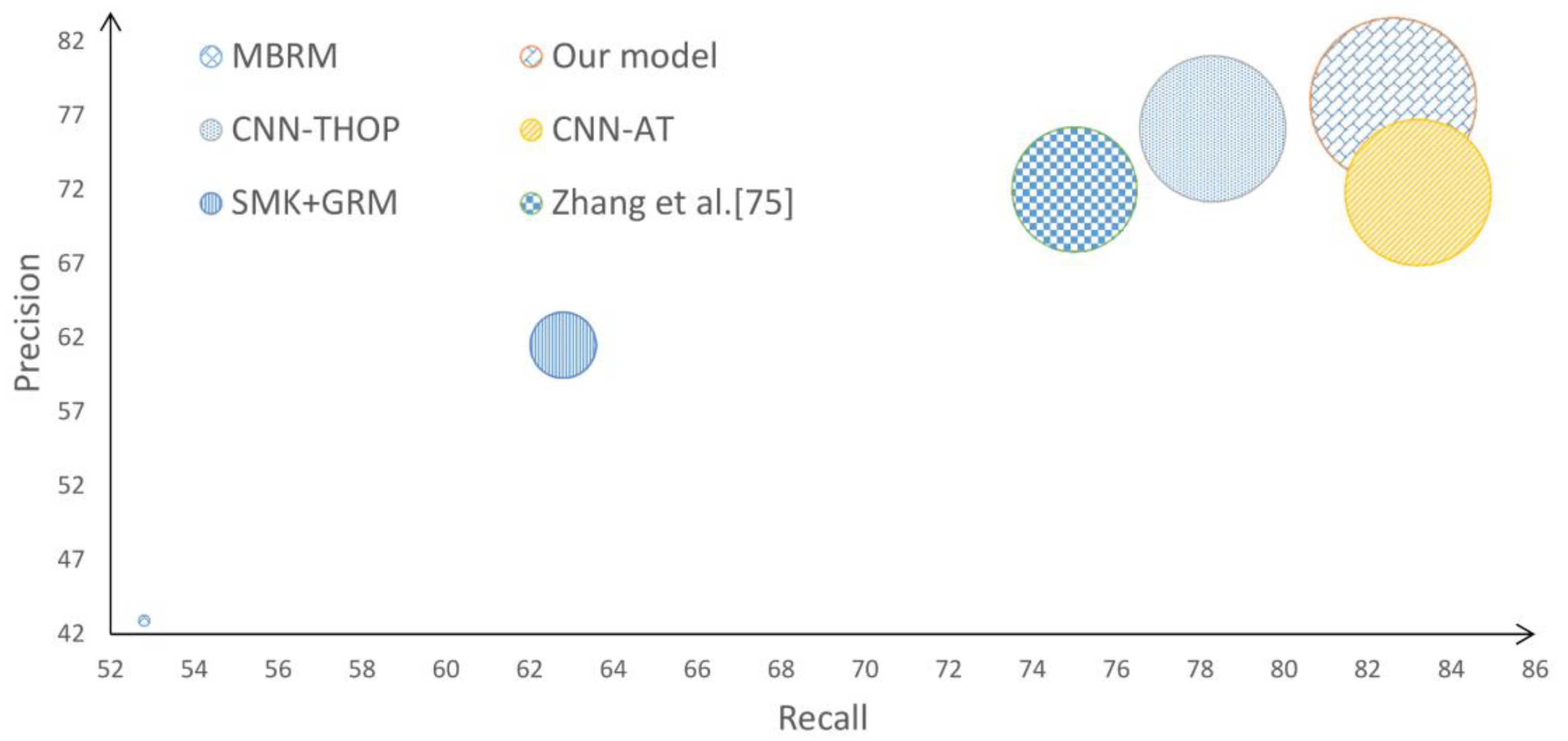
4.3. Scenario 2: Comparing Our Method to the State of the Art

In this second scenario, our proposed method has been compared to a wide range of AIA methods in the literature. For the sake of clarity, these methods have been categorized into region-based and holistic-based, each of which contains CNN- and handcrafted-based features [46]. It is worth noting that some works in literature use the full set of dataset’s annotations (e.g., 374 concepts for Corel-5K), whereas some others pick only a subset of 260 concepts. In our experiments, however, we engaged both two scenarios: 374 and 260 concepts. One must know that a good AIA system should achieve equivalence in the proportion of correctly assigning different concepts. In other words, the standard deviation of correctly assigning concepts needs to be minimized. Unfortunately, we were not able to find statistics, such as standard deviations and medians, about the obtained results in most of the related works for comparison.

Corel-5K has had the major share of experiments for AIA tasks. Since there are many related works for which there is no room to mention here, we have involved the more recent ones in our comparison (those proposed after 2015).

Table 2. A comparison between our method and other recent related works in terms of precision (P), recall (R), F1, and N+. The involved works adopt one of the following scenarios: considering 260 concepts or considering 374 concepts, as shown in the ‘No. Cpt’ column.

	Method	No. Cpt	P	R	F1	N+
Holistic approach	CNN-R (2015) [7]	374	32	41.3	36.1	166
	KCCA (2015) [7]	374	39	53	44.9	184
	CCA-KNN (2015) [7]	374	42	52	46.5	201
	Group Sparsity (2015) [47]	260	30	33	31.4	146
	GLKNN (2015) [48]	260	36	47	40.8	184
	MIAPS (2015) [49]	260	39.98	42.66	41.28	177
	MVSAE (2015) [50]	260	37	47	42	175
	LJNMF (2015) [51]	260	35	43	39.1	175
	SLED (2015) [52]	260	35	51	41.5	-
	AWD-IKNN (2016) [53]	260	42	55	47.7	198
	CNN-AT (2016) [54]	374	26	17	21	88
	NSIDML (2016) [55]	260	44.12	51.76	47.76	194
	MLDL (2016) [56]	260	45	49	47	198
	LDMKL (2017) [57]	200	29	44	35	179
	SDMKL (2017) [57]	200	25	38		158
	L-ADA (2017) [58]	260	31	38	34	164
	NL-ADA (2017) [58]	260	32	40	36	173
	MVG-NMF (2017) [59]	260	44	47.5	45.6	197
	PRM (2017) [60]	260	40.78	53.64	46.33	205
	VSE-2PKNN-ML (2018) [61]	260	41	52	46	205
	PRM DEEP (2018) [62]	260	45.3	51.73	48.3	201
	CCAKNN (2018) [63]	260	41	43	42	185
	IDFRW (2018) [64]	260	38	49	43	185
	CDNI (2018) [65]	260	29.8	32.1	30.9	162
	OPSL (2018) [66]	260	38.3	55	45.2
	E2E-DCNN (2019) [67]	260	41	55	47	192
	SEM (2019) [68]	260	37	52	43	-
	L-Global CA (2019) [69]	260	36	45		189
	S-Global CA (2019) [69]	260	36	46		194
	L-Classwise CA (2019) [69]	260	36	45		192
	LL-PLSA (2020) [70]	260	37	48	42	-
	RDPGKNN (2020) [71]	260	40	45	40	195
	Weight-KNN (2020) [23]	260	22	15	18	-
	Khatchatoorian et al. (2020) [72]	260	55.46	56.55	56	212
	GCN (2020) [73]	260	48	52	49	200
	CNN-THOP (2020) [74]	260	52.7	58.3	55.3	-
	SSGL (2020) [75]	260	34	47	40	190
	Zhang et al. (2020) [76]	374	60	68	64	228
	PLSA-MB (2020) [77]	260	26	30	27.9
	TAIA (2020) [78]	260	38.4	48.6	42.9	177
	Y.chen et al. (2021) [79]	260	26.93	41.43	32.64	161
	TSEM (2021) [80]	260	38	46	42	-
	TSEM+LQP (2021) [80]	260	45	40	43	-
	SSL-AWF (2021) [81]	260	51	48	49.5	203
	CNN-SPP (2021) [81]	260	46	43	44.4	196
	HMAA (2021) [1]	260	43	54	48
	MVRSC (2021) [82]	260	54.3	42.9	47.9
	LDA-ECC (2021) [81]	260	35	36	35.5	148
Region-based approach	MLSIA (2015) [19]	374	23.35	26.24	23.54	-
	ANNOR-G (2015) [83]	260	22	29	25	129
	Zhang et al. (2016) [16]	374	57.61	53.04	53.85	-
	BG (2019) [84]	374	33	41		170
	TG (2019) [84]	374	36	45		189
	Vatani et al. (2020) [85]	260	28	96	43	-
	Our method	374	48.63	64.94	54.85	236
	Our method	260	59.45	65.01	58.89	212

presents results obtained from our method compared to those of the related works using the Corel-5K dataset.

From Table 2, it appears that our proposed segmentation-based AIA method outperforms the majority of the stated related works in both scenarios of 274 and 260 concepts. If we take as an instance the top two F1 scores yielded by the related works Khatchatoorian et al. (2020) [72] and CNN-THOP (2020) [74] in the scenario of 260 concepts, we can clearly see that the outcomes of our method exceed those of both methods by 5% at least. Furthermore, the F1 score obtained by our method is at least 10% higher than that obtained by other recent studies such as GCN (2020) [73], SSL-AWF (2021) [81], and MVRSC (2021) [82]. Now, if we look at the scenario of 374 concepts, we can see that our proposed method has surpassed all other methods except for that of Vatani et al. (2020) [85]. However, if we consider the method of Vatani et al. in terms of N+, we can see that our method outperforms it by eight concepts. This means that our method is capable of appropriately assigning eight more concepts than the method of Vatani et al. As previously said, it is not sufficient for a technique to achieve high accuracy alone; it should also acquire the meaning of the greatest number possible of concepts.

To further analyze the outcomes of our method, we have calculated statistics of P, R, and F1 and presented them using a box plot. Figure 7 presents some statistics about how our proposed method learns the meaning of concepts.

From the first glance, it appears that there is a compromise between precision and recall based on the used number of concepts. With 374 concepts, for instance, our system achieved a recall that is far higher than the precision. When it comes to 260 concepts, however, the precision remarkably improved whereas the recall slightly decreased. As the depicted standard deviation (≈14 in both cases) indicates, our proposed technique aids in the balanced learning of various concepts. With a median of 45.7 in the scenario of 374 concepts, our findings indicate that more than half of the images were annotated with at least two to three accurate concepts, which is a significant number given a large number of concepts (374 concepts). Nonetheless, the number of correctly annotated images with two to three concepts increases substantially in the case of 260 images, resulting in a 75% rate. It should be noted that manually annotating images involves some subjectivity or mistakes, which results in the appearance of certain outliers, as seen in Figure 7.

On one hand, the approach proposed in the work of Zhang et al. (2016) [16] relies totally on finding the semantic relatedness among presegmented regions based on a wide range of handcrafted features [86,87]. By understanding the logic that connects different concepts, the system became able to learn concepts regardless of their narrow use. On the other hand, the idea in the work of Khatchatoorian et al. (2020) [72] revolves around employing CNN as a black box and letting it learn everything by itself. However, we have taken advantage of both the methods by applying a CNN to obtain a rich set of features representing the concepts and employing KNN regression to understand how these concepts are related. By doing so, we have exceeded the performance of both previous techniques.

MSRC v2 dataset has also been used to assist the performance of AIA systems in various literature works, in particular those based on regions. We have conducted a comparison against some recent works on the same dataset using the same 22-concept scenario. Due to the limited number of annotations (22 concepts only), the metric N+ has been disregarded in this comparison since it always produces the perfect result (i.e., N+ = 22). Figure 8 presents F1 in terms of precision and recall using the MSRC v2 dataset.

Figure 8 clearly shows that our proposed method outperforms the others by yielding precision = 78.01% and recall = 82.6% which produce the highest F1 score of 80.24%. However, assessing the method’s performance based on a sample mean of precisions is, in many cases, deceptive. Therefore, it is a common practice in AIA performance assessment procedure to evaluate the performance on each concept individually. Figure 9 presents a precision heatmap yielded by our method compared to the others.

As it appears from Figure 9, CNN-THOP and our method have outperformed the others by yielding perfect precisions with four concepts. Furthermore, our method has achieved more than 0.98 for another three concepts, namely grass, airplane, and bike. If we take the third quantile for both methods (≈0.93 for CNN-THOP and ≈0.99 for our method) as an example, we can deduce that far more concepts have been appropriately grasped by our method than by CNN-THOP. Furthermore, our approach has a standard deviation of 0.7, whereas CCN-THOP has a standard deviation of 0.14, indicating that the former has a better balance in learning concepts, whilst the latter only concentrates on a few of them. The outcomes of this experiment prove that guiding a CNN-based AIA system through a preprocessing of image segmentation could highly improve the results.

Poor performance of an AIA system does not always reflect inefficiency; in many cases, it is a result of a poorly annotated dataset. To further clarify this last argument, we have collected some images in which the ground truth does not accurately reflect the content of the image.

Table 3. A list of images with their respective ground truths and given annotations. Concepts in bold indicate that they are parts of the ground truth.

	Ground Truth	CMRM [26]	Our Method
1.	car, tracks, grass	water, tree, sky, people, grass	car, tracks, turn, prototype
2.	sky, tree, castle	people, building, ohau, water, tree	sky, clouds, tree, house
3.	flowers, petals, leaf	sky, water, people, tree, grass	leaf, flowers, petals, stems
4.	flowers, tree, sky	flowers, tree, grass, lawn, sky	sky, tree, flower, tulip
5.	sky, plane, runway	plane, jet, sky, cars, tracks	plane, runway, prop

shows a list of test images with their respective ground truths and annotations given by AIA systems.

Table 3 shows that, compared to the ground truth, some annotations have been indeed assigned, some have been replaced with their synonyms, and some others have been completely omitted. If we take image number 3 as an example, we can see that the precision of the annotation process is 50% (i.e., two out of three concepts from the ground truth have been assigned to the image by the AIA). However, a careful inspection reveals that all the assigned concepts do indeed describe the image (image 2 contains clouds and a house). The same goes for the rest of the images.

4.4. Scenario 3: Computing Cost

When an algorithm is dedicated to being utilized with entities with restricted sources of power or poor processing capacity, its speed is an essential factor in determining its performance. In this experiment, we evaluate and compare our method to other common AIA methods in terms of time consumed in the annotation process.

Table 4. Time consumed, in seconds, for annotating one image with five concepts.

	Our Method	SKL-CRM [91]	MLDL [56]	2PKNN [11]	TagProp [6]
Consumed time	1.2	27	24.6	0.6	0.6

shows the result of comparing our method to other famous methods in terms of time consumption during annotation.

From Table 4, it appears that our method has a relatively acceptable time for annotating images. This can be attributed to the simple scheme we adopt that does not require complicated calculations such as those required for MLDL [55] and SKL-CRM [91]. This is because the present method places a strong emphasis on speed and minimal computation, which can be proved by the used sample region growing JSEG algorithm for image segmentation and off-the-shelf features extracted from the fastest network MobileNet that is dedicated for mobiles. The pretrained CNN is employed in a manner that does not require any further training or finetuning, which reduces the amount of computing needed. These criteria grant rapidity and low consumption of resources and make our method suitable for mobiles or other small entities.

5. Conclusions

This paper introduced an automatic image annotation system in which segmentation JSEG algorithm, a convolutional neural network named MobileNet, and KNN regression methods have been employed. MobileNet has been adopted to grant a rich representation of regions generated by JSEG, and KNN regressor is employed to understand how these concepts are related. After tuning the best values of our method, it has been compared against other methods in terms of precision, recall, F1, N+, and computing time. The two common scenarios of 374 and 260 concepts have been taken into account for the dataset Corel-5K. F1 of 54.85% and N+ of 236 for the first scenario and F1 of 58.89% and N+ of 212 for the second scenario have been achieved. These results indicate the superiority of the proposed approach compared to a wide range of related works. Furthermore, a statistical analysis has been carried out on the outcoming of our method and has proved that our proposed method aids in more balanced learning of different concepts. To further prove the superiority of our method, it has been compared against other region-based works on the MSRC v2 dataset. Results proved that the concepts corresponding to the third quartile achieve more than 99% precision, which is an important amount of concepts. Since the present method places a strong emphasis on speed and minimal computation, we compared it against other common methods in terms of time consumption. Results proved its rapidity and low consumption of resources which make it suitable for mobiles or other small entities. The experiments also demonstrated that the precision yielded by our method is somewhat biased due to the poor quality of the ground truth. Therefore, our method should be exploited in enhancing the ground truth of manually annotated datasets by eliminating the problems of missing data and noise.

References

1. Chen, J.; Ying, P.; Fu, X.; Luo, X.; Guan, H.; Wei, K. Automatic tagging by leveraging visual and annotated features in social media. IEEE Trans. Multimed. 2021, 9210, 1–12. [Google Scholar]
2. Stangl, A.; Morris, M.R.; Gurari, D. Person, Shoes, Tree. Is the Person Naked? What People with Vision Impairments Want in Image Descriptions. In Proceedings of the 2020 CHI Conference on Human Factors in Computing Systems, Honolulu, HI, USA, 25–30 April 2020; pp. 1–13. [Google Scholar]
3. Ben, H.; Pan, Y.; Li, Y.; Yao, T.; Hong, R.; Wang, M.; Mei, T. Unpaired Image Captioning with Semantic-Constrained Self-Learning. IEEE Trans. Multimed. 2021, 1. [Google Scholar] [CrossRef]
4. Moran, S.; Lavrenko, V. Sparse kernel learning for image annotation. In Proceedings of the ICMR 2014—ACM International Conference on Multimedia Retrieval 2014, Glasgow, UK, 1–4 April 2014; pp. 113–120. [Google Scholar]
5. Zhang, S.; Huang, J.; Li, H.; Metaxas, D.N. Automatic image annotation and retrieval using group sparsity. IEEE Trans. Syst. Man Cybern. Part B Cybern. 2012, 42, 838–849. [Google Scholar] [CrossRef]
6. Guillaumin, M.; Mensink, T.; Verbeek, J.; Schmid, C. TagProp: Discriminative metric learning in nearest neighbor models for image auto-annotation. In Proceedings of the IEEE 12th International Conference on Computer Vision, Kyoto, Japan, 29 September–2 October 2009; pp. 309–316. [Google Scholar]
7. Murthy, V.N.; Maji, S.; Manmatha, R. Automatic image annotation using deep learning representations. In Proceedings of the ICMR 2015—5th ACM on International Conference on Multimedia Retrieval, Shanghai, China, 23–26 June 2015; pp. 603–606. [Google Scholar]
8. Murthy, V.N.; Can, E.F.; Manmatha, R. A hybrid model for automatic image annotation. In Proceedings of the ICMR 2014—ACM International Conference on Multimedia Retrieval 2014, Glasgow, UK, 1–4 April 2014; pp. 369–376. [Google Scholar]
9. Makadia, A.; Pavlovic, V.; Kumar, S. A new baseline for image annotation. In Lecture Notes in Computer Science (LNCS); Springer: Berlin/Heidelberg, Germany, 2008; Volume 5304, pp. 316–329. [Google Scholar]
10. Xiang, Y.; Zhou, X.; Chua, T.S.; Ngo, C.W. A revisit of generative model for automatic image annotation using markov random fields. In Proceedings of the 2009 IEEE Conference on Computer Vision and Pattern Recognition Work (CVPR Work), Miami, FL, USA, 20–25 June 2009; Volume 2009, pp. 1153–1160. [Google Scholar]
11. Verma, Y.; Jawahar, C.V. Image Annotation Using Metric Learning in Semantic Neighbourhoods. In Lecture Notes in Computer Science; Springer: Berlin/Heidelberg, Germany, 2012; pp. 836–849. [Google Scholar]
12. Verma, Y.; Jawahar, C.V. Exploring SVM for image annotation in presence of confusing labels. In Proceedings of the BMVC 2013—British Machine Vision Conference, BMVC 2013, Bristol, UK, 9–13 September 2013. [Google Scholar]
13. Yang, C.; Dong, M.; Hua, J. Region-based image annotation using asymmetrical support vector machine-based multiple-instance learning. Proc. IEEE Comput. Soc. Conf. Comput. Vis. Pattern Recognit. 2006, 2, 2057–2063. [Google Scholar]
14. Wang, Y.; Mei, T.; Gong, S.; Hua, X.S. Combining global, regional and contextual features for automatic image annotation. Pattern Recognit. 2009, 42, 259–266. [Google Scholar] [CrossRef]
15. Rejeb, I.B.; Ouni, S.; Barhoumi, W.; Zagrouba, E. Fuzzy VA-Files for multi-label image annotation based on visual content of regions. Signal Image Video Process. 2018, 12, 877–884. [Google Scholar] [CrossRef]
16. Zhang, J.; Gao, Y.; Feng, S.; Yuan, Y.; Lee, C.H. Automatic image region annotation through segmentation based visual semantic analysis and discriminative classification. In Proceedings of the 2016 IEEE International Conference on Acoustics, Speech and Signal Processing (ICASSP), Shanghai, China, 20–25 March 2016; Volume 2016, pp. 1956–1960. [Google Scholar]
17. Yuan, J.; Li, J.; Zhang, B. Exploiting spatial context constraints for automatic image region annotation. Proc. ACM Int. Multimed. Conf. Exhib. 2007, 595–604. [Google Scholar] [CrossRef] [Green Version]
18. Zhang, J.; Mu, Y.; Feng, S.; Li, K.; Yuan, Y.; Lee, C. Image region annotation based on segmentation and semantic correlation analysis. IET Image Process. 2018, 12, 1331–1337. [Google Scholar] [CrossRef]
19. Zhang, J.; Zhao, Y.; Li, D.; Chen, Z.; Yuan, Y. A novel image annotation model based on content representation with multi-layer segmentation. Neural Comput. Appl. 2015, 26, 1407–1422. [Google Scholar] [CrossRef]
20. Chen, Y.; Zeng, X.; Chen, X.; Guo, W. A survey on automatic image annotation. Appl. Intell. 2020, 50, 3412–3428. [Google Scholar] [CrossRef]
21. Jerhotová, E.; Švihlík, J.; Procházka, A. Biomedical Image Volumes Denoising via the Wavelet Transform. In Applied Biomedical Engineering; Gargiulo, G.D., McEwan, A., Eds.; IntechOpen: London, UK, 2011; pp. 435–458. [Google Scholar] [CrossRef] [Green Version]
22. Bnou, K.; Raghay, S.; Hakim, A. A wavelet denoising approach based on unsupervised learning model. EURASIP J. Adv. Signal Process. 2020, 2020, 36. [Google Scholar] [CrossRef]
23. Ma, Y.; Xie, Q.; Liu, Y.; Xiong, S. A weighted KNN-based automatic image annotation method. Neural Comput. Appl. 2020, 32, 6559–6570. [Google Scholar] [CrossRef]
24. Carneiro, G.; Vasconcelos, N. Formulating semantic image annotation as a supervised learning problem. Proc. IEEE Comput. Soc. Conf. Comput. Vis. Pattern Recognit. 2005, II, 163–168. [Google Scholar]
25. Blei, D.M.; Jordan, M.I. Modeling annotated data. In Proceedings of the 26th ACM/SIGIR International Symposium on Information Retrieval, Toronto, ON, Canada, 28 July–1 August 2003; p. 127. [Google Scholar]
26. Li, L.J.; Socher, R.; Fei-Fei, L. Towards total scene understanding: Classification, annotation and segmentation in an automatic framework. IEEE Comput. Soc. Conf. Comput. Vis. Pattern Recognit. Work 2009, 2009, 2036–2043. [Google Scholar]
27. Brown, P.F.; Pietra, S.D.; Pietra, V.J.D.; Mercer, R.L. The Mathematics of Statistical Machine Translation: Parameter Estimation. Comput. Linguist. 1994, 19, 263–311. [Google Scholar]
28. Jeon, J.; Lavrenko, V.; Manmatha, R. Automatic Image Annotation and Retrieval using Cross-Media Relevance Models. In Proceedings of the 26th ACM/SIGIR International Symposium on Information Retrieval, Toronto, ON, Canada, 28 July–1 August 2003; pp. 119–126. [Google Scholar]
29. Feng, S.L.; Manmatha, R.; Lavrenko, V. Multiple Bernoulli relevance models for image and video annotation. Proc. IEEE Comput. Soc. Conf. Comput. Vis. Pattern Recognit. 2004, 2, 1002–1009. [Google Scholar]
30. Chen, B.; Li, J.; Lu, G.; Yu, H.; Zhang, D. Label Co-Occurrence Learning With Graph Convolutional Networks for Multi-Label Chest X-Ray Image Classification. IEEE J. Biomed. Health Inform. 2020, 24, 2292–2302. [Google Scholar] [CrossRef] [PubMed]
31. Mori, Y.; Takahashi, H.; Oka, R. Image-to-Word Transformation Based on Dividing and Vector Quantizing Images with Words; CiteSeerX: Princeton, NJ, USA, 1999. [Google Scholar]
32. Duygulu, P.; Barnard, K.; de Freitas, J.F.G.; Forsyth, D.A. Object recognition as machine translation: Learning a lexicon for a fixed image vocabulary. In Lecture Notes in Computer Science; Springer: Berlin/Heidelberg, Germany, 2002; Volume 2353, pp. 97–112. [Google Scholar]
33. Barnard, K.; Duygulu, P.; Forsyth, D.; de Freitas, N.; Blei, D.M.; Jordan, M.I. Matching words and pictures. J. Mach. Learn. Res. 2003, 3, 1107–1135. [Google Scholar]
34. Darwish, S.M. Combining firefly algorithm and Bayesian classifier: New direction for automatic multilabel image annotation. IET Image Process. 2016, 10, 763–772. [Google Scholar] [CrossRef]
35. Gould, S.; Fulton, R.; Koller, D. Decomposing a scene into geometric and semantically consistent regions. Proc. IEEE Int. Conf. Comput. Vis. 2009, 1–8. [Google Scholar] [CrossRef] [Green Version]
36. Bhagat, P.; Choudhary, P. Image Annotation: Then and Now, Image and Vision Computing; Elsevier: Amsterdam, The Netherlands, 2018; Volume 80, pp. 1–23. [Google Scholar]
37. Deng, Y.; Manjunath, B.; Shin, H. Color image segmentation. In Proceedings of the 1999 IEEE Computer Society Conference on Computer Vision and Pattern Recognition (Cat. No PR00149), Fort Collins, CO, USA, 23–25 June 1999; Volume 2, pp. 446–451. [Google Scholar]
38. Khattab, D.; Ebied, H.M.; Hussein, A.S.; Tolba, M.F. Color image segmentation based on different color space models using automatic GrabCut. Sci. World J. 2014, 2014, 126025. [Google Scholar] [CrossRef]
39. Aloun, M.S.; Hitam, M.S.; Yussof, W.N.H.W.; Hamid, A.A.K.A.; Bachok, Z. Modified JSEG algorithm for reducing over-segmentation problems in underwater coral reef images. Int. J. Electr. Comput. Eng. 2019, 9, 5244–5252. [Google Scholar] [CrossRef]
40. Oquab, M.; Bottou, L.; Laptev, I.; Sivic, J. Learning and transferring mid-level image representations using convolutional neural networks. Proc. IEEE Comput. Soc. Conf. Comput. Vis. Pattern Recognit. 2014, 1717–1724. [Google Scholar] [CrossRef] [Green Version]
41. Zeiler, M.D.; Fergus, R. Visualizing and understanding convolutional networks. In Lecture Notes in Computer Science; Springer: Berlin/Heidelberg, Germany, 2014; Volume 8689, pp. 818–833. [Google Scholar]
42. Howard, A.G.; Zhu, M.; Chen, B.; Kalenichenko, D.; Wang, W.; Weyand, T.; Andreetto, M.; Adam, H. MobileNets: Efficient Convolutional Neural Networks for Mobile Vision Applications. arXiv 2017, arXiv:1704.04861. [Google Scholar]
43. Lai, S.; Zhu, Y.; Jin, L. Encoding Pathlet and SIFT Features With Bagged VLAD for Historical Writer Identification. IEEE Trans. Inf. Forensics Secur. 2020, 15, 3553–3566. [Google Scholar] [CrossRef]
44. McConville, R.; Santos-Rodriguez, R.; Piechocki, R.J.; Craddock, I. N2D: (not too) deep clustering via clustering the local manifold of an autoencoded embedding. Proc. Int. Conf. Pattern Recognit. 2020, 5145–5152. [Google Scholar] [CrossRef]
45. Khaldi, B.; Aiadi, O.; Kherfi, M.L. Combining colour and greylevel cooccurrence matrix features: A comparative study. IET Image Process. 2019, 13, 1401–1410. [Google Scholar] [CrossRef]
46. Khaldi, B.; Aiadi, O.; Lamine, K.M. Image representation using complete multi-texton histogram. Multimed. Tools Appl. 2020, 79, 8267–8285. [Google Scholar] [CrossRef]
47. Zhang, X.; Liu, C. Image annotation based on feature fusion and semantic similarity. Neurocomputing 2015, 149, 1658–1671. [Google Scholar] [CrossRef]
48. Su, F.; Xue, L. Graph Learning on K Nearest Neighbours for Automatic Image Annotation. In Proceedings of the ICMR 2015—5th ACM on International Conference on Multimedia Retrieval, Shanghai, China, 23–26 June 2015; pp. 403–410. [Google Scholar]
49. Amiri, S.H.; Jamzad, M. Efficient multi-modal fusion on supergraph for scalable image annotation. Pattern Recognit. 2015, 48, 2241–2253. [Google Scholar] [CrossRef]
50. Yang, Y.; Zhang, W.; Xie, Y. Image automatic annotation via multi-view deep representation. J. Vis. Commun. Image Represent. 2015, 33, 368–377. [Google Scholar] [CrossRef]
51. Rad, R.; Jamzad, M. Automatic image annotation by a loosely joint non-negative matrix factorisation. IET Comput. Vis. 2015, 9, 806–813. [Google Scholar] [CrossRef]
52. Cao, X.; Zhang, H.; Guo, X.; Liu, S.; Meng, D. SLED: Semantic Label Embedding Dictionary Representation for Multilabel Image Annotation. IEEE Trans. Image Process. 2015, 24, 2746–2759. [Google Scholar]
53. Li, J.; Yuan, C. Automatic Image Annotation Using Adaptive Weighted Distance in Improved K Nearest Neighbors Framework. In Pacific Rim Conference on Multimedia; Springer: Cham, Switzerland, 2016; Volume 2, pp. 345–354. [Google Scholar]
54. Le, H.M.; Nguyen, T.-O.; Ngo-Tien, D. Fully Automated Multi-label Image Annotation by Convolutional Neural Network and Adaptive Thresholding. In Proceedings of the Seventh Symposium on Information and Communication Technology, Ho Chi Minh City, Vietnam, 8–9 December 2016. [Google Scholar]
55. Jin, C.; Jin, S.-W. Image distance metric learning based on neighborhood sets for automatic image annotation, Journal of Visual Communication and Image Representation. J. Vis. Commun. Image Represent. 2016, 34, 167–175. [Google Scholar] [CrossRef]
56. Jing, X.-Y.; Wu, F.; Li, Z.; Hu, R.; Zhang, D. Multi-Label Dictionary Learning for Image Annotation. IEEE Trans. Image Process. 2016, 25, 2712–2725. [Google Scholar] [CrossRef]
57. Jiu, M.; Sahbi, H. Nonlinear Deep Kernel Learning for Image Annotation. IEEE Trans. Image Process. 2017, 26, 1820–1832. [Google Scholar] [CrossRef] [PubMed]
58. Ke, X.; Zhou, M.; Niu, Y.; Guo, W. Data equilibrium based automatic image annotation by fusing deep model and semantic propagation. Pattern Recognit. 2017, 71, 60–77. [Google Scholar] [CrossRef]
59. Rad, R.; Jamzad, M. Image annotation using multi-view non-negative matrix factorization with different number of basis vectors. J. Vis. Commun. Image Represent. 2017, 46, 1–12. [Google Scholar] [CrossRef]
60. Khatchatoorian, A.G. Post rectifying methods to improve the accuracy of image annotation. In Proceedings of the International Conference on Digital Image Computing: Techniques and Applications (DICTA), Sydney, NSW, Australia, 29 November–1 December 2017; pp. 406–412. [Google Scholar]
61. Zhang, W.; Hu, H.; Hu, H. Training Visual-Semantic Embedding Network for Boosting Automatic Image Annotation. Neural Process. Lett. 2018, 48, 1503–1519. [Google Scholar] [CrossRef]
62. Khatchatoorian, A.G.; Jamzad, M. An Image Annotation Rectifying Method Based on Deep Features. In Proceedings of the 2018 2nd International Conference on Digital Signal Processing, Tokyo, Japan, 25–27 February 2018; pp. 88–92. [Google Scholar]
63. Wang, X.L.; Hongwei, G.E.; Liang, S. Image automatic annotation algorithm based on canonical correlation analytical subspace and k-nearest neighbor. J. Ludong Univ. 2018. [Google Scholar]
64. Ning, Z.; Zhou, G.; Chen, Z.; Li, Q. Integration of image feature and word relevance: Toward automatic image annotation in cyber-physical-social systems. IEEE Access 2018, 6, 44190–44198. [Google Scholar] [CrossRef]
65. Maihami, V.; Yaghmaee, F. Automatic image annotation using community detection in neighbor images. Phys. A Stat. Mech. Its Appl. 2018, 507, 123–132. [Google Scholar] [CrossRef]
66. Xue, Z.; Li, G.; Huang, Q. Joint multi-view representation and image annotation via optimal predictive subspace learning. Inf. Sci. 2018, 451–452, 180–194. [Google Scholar] [CrossRef]
67. Ke, X.; Zou, J.; Niu, Y. End-to-End Automatic Image Annotation Based on Deep CNN and Multi-Label Data Augmentation. IEEE Trans. Multimed. 2019, 21, 2093–2106. [Google Scholar] [CrossRef]
68. Ma, Y.; Liu, Y.; Xie, Q.; Li, L. CNN-feature based automatic image annotation method. Multimed. Tools Appl. 2019, 78, 3767–3780. [Google Scholar] [CrossRef]
69. Jiu, M.; Sahbi, H. Deep Context-Aware Kernel Networks. arXiv 2019, arXiv:1912.12735. [Google Scholar]
70. Song, H.; Wang, P.; Yun, J.; Li, W.; Xue, B.; Wu, G. A Weighted Topic Model Learned from Local Semantic Space for Automatic Image Annotation. IEEE Access 2020, 8, 76411–76422. [Google Scholar] [CrossRef]
71. Chen, S.; Wang, M.; Chen, X. Communications, Mobilenbsp;, and 2020, Image annotation via reconstitution graph learning model. Wirel. Commun. Mob. Comput. 2020, 2020, 1–9. [Google Scholar]
72. Khatchatoorian, A.G.; Jamzad, M. Architecture to improve the accuracy of automatic image annotation systems. IET Comput. Vis. 2020, 14, 214–223. [Google Scholar] [CrossRef]
73. Zhu, Z.; Hangchi, Z. Image annotation method based on graph volume network. In Proceedings of the 2020 International Conference on Intelligent Transportation, Big Data & Smart City, ICITBS 2020, Vientiane, Laos, 11–12 January 2020; pp. 885–888. [Google Scholar]
74. Cao, J.; Zhao, A.; Zhang, Z. Automatic image annotation method based on a convolutional neural network with threshold optimization. PLoS ONE 2020, 15, e0238956. [Google Scholar] [CrossRef]
75. Chen, Z.; Wang, M.; Gao, J.; Li, P. Image Annotation based on Semantic Structure and Graph Learning. In Proceedings of the IEEE Intl Conf on Dependable, Autonomic and Secure Computing, Intl Conf on Pervasive Intelligence and Computing, Intl Conf on Cloud and Big Data Computing, Intl Conf on Cyber Science and Technology Congress, Calgary, AB, Canada, 17–22 August 2020; pp. 451–456. [Google Scholar]
76. Zhang, W.; Hu, H.; Hu, H.; Yu, J. Automatic image annotation via category labels. Multimed. Tools Appl. 2020, 79, 11421–11435. [Google Scholar] [CrossRef]
77. Tian, D.; Shi, Z. A two-stage hybrid probabilistic topic model for refining image annotation. Int. J. Mach. Learn. Cybern. 2019, 11, 417–431. [Google Scholar] [CrossRef]
78. Ge, H.; Zhang, K.; Hou, Y.; Yu, C.; Zhao, M.; Wang, Z.; Sun, L. Two-stage Automatic Image Annotation Based on Latent Semantic Scene Classification. In Proceedings of the International Joint Conference on Neural Networks (IJCNN), Glasgow, UK, 19–24 July 2020. [Google Scholar]
79. Chen, Y.; Liu, L.; Tao, J.; Chen, X.; Xia, R.; Zhang, Q.; Xiong, J.; Yang, K.; Xie, J. The image annotation algorithm using convolutional features from intermediate layer of deep learning. Multimed. Tools Appl. 2020, 80, 4237–4261. [Google Scholar] [CrossRef]
80. Wei, W.; Wu, Q.; Chen, D.; Zhang, Y.; Liu, W.; Duan, G.; Luo, X. Automatic image annotation based on an improved nearest neighbor technique with tag semantic extension model. Procedia Comput. Sci. 2021, 183, 616–623. [Google Scholar] [CrossRef]
81. Li, Z.; Lin, L.; Zhang, C.; Ma, H.; Zhao, W.; Shi, Z. A Semi-supervised Learning Approach Based on Adaptive Weighted Fusion for Automatic Image Annotation. ACM Trans. Multimedia Comput. Commun. Appl. 2021, 17, 1–23. [Google Scholar]
82. Zamiri, M.; Yazdi, H.S. Image annotation based on multi-view robust spectral clustering. J. Vis. Commun. Image Represent. 2020, 74, 103003. [Google Scholar] [CrossRef]
83. Kuric, E.; Bielikova, M. ANNOR: Efficient Image Annotation Based on Combining Local and Global Features. Comput. Graph. 2016, 47, 1–15. [Google Scholar] [CrossRef]
84. Zhang, J.; Tao, T.; Mu, Y.; Sun, H.; Li, D.; Wang, Z. Web image annotation based on Tri-relational Graph and semantic context analysis. Eng. Appl. Artif. Intell. 2019, 81, 313–322. [Google Scholar] [CrossRef]
85. Vatani, A.; Ahvanooey, M.T.; Rahimi, M. An effective automatic image annotation model via attention model and data equilibrium. Int. J. Adv. Comput. Sci. Appl. 2001, 9, 269–277. [Google Scholar] [CrossRef] [Green Version]
86. Kaoudja, Z.; Kherfi, M.L.; Khaldi, B. An efficient multiple-classifier system for Arabic calligraphy style recognition. In Proceedings of the International Conference on Networking and Advanced Systems (ICNAS), Annaba, Algeria, 26–27 June 2019. [Google Scholar]
87. Aiadi, O.; Kherfi, M.L.; Khaldi, B. Automatic Date Fruit Recognition Using Outlier Detection Techniques and Gaussian Mixture Models. ELCVIA Electron. Lett. Comput. Vis. Image Anal. 2019, 18, 52–75. [Google Scholar] [CrossRef]
88. Lu, Z.; Ip, H.H. Generalized relevance models for automatic image annotation. In Lecture Notes in Computer Science; Springer: Berlin/Heidelberg, Germany, 2009; Volume 5879, pp. 245–255. [Google Scholar]
89. Lu, Z.; Ip, H.H.; He, Q. Context-based multi-label image annotation. In Proceedings of the International Conference on Image and Video Retrieval Santorini, Fira, Greece, 8–10 July 2009. [Google Scholar]
90. Li, Z.; Zheng, Y.; Zhang, C.; Shi, Z. Combining Deep Feature and Multi-label Classification for Semantic Image Annotation. J. Comput. Des. Comput. Graph. 2018, 30, 318. [Google Scholar]
91. Moran, S.; Lavrenko, V. sparse kernel relevance model for automatic image annotation. Int. J. Multimedia Inf. Retr. 2014, 3, 209–229. [Google Scholar] [CrossRef]
Figure 1. The different phases that constitute our proposed AIA approach. Black solid arrows correspond to training images, whereas the blue ones correspond to test images. All images pass through a segmentation phase using JSEG algorithm, the segmented regions are fed to a CNN for feature extraction, features are encoded, a codebook is generated, and then KNN regression is employed to link blobs with labels and assign new labels.
Applsci 11 10176 g001
Figure 2. A general scheme of texture-enhanced JSEG (T-JSEG) segmentation method. At the preprocessing level, the HSV color space is firstly quantized and all pixels of the image are then mapped to their corresponding bins. At the segmentation level, the J-image and a class map for each windowed color region are calculated, and then a clustering/growing algorithm is applied to obtain distinct regions.
Applsci 11 10176 g002
Figure 3. MobileNet architecture.
Applsci 11 10176 g003
Figure 4. Precision and recall yielded using the three aggregation methods: BoVF, VLAD, and FV.
Applsci 11 10176 g004
Figure 5. The impact of changing the value of K of KNN regressor on (a) the precision and (b) the recall of our proposed method.
Applsci 11 10176 g005
Figure 6. The impact of using different CNN models on our proposed method. The impact is measured in terms of precision, recall, and complexity.
Applsci 11 10176 g006
Figure 7. Statistical description of how our proposed method learns the meanings of concepts accurately and in a balanced manner. Precision and recall are denoted by the letters P and R, respectively, and the following number denotes the number of concepts utilized in the experiment.
Applsci 11 10176 g007
Figure 8. A blob chart of F1 in terms of precision and recall. The experiments were conducted on MSRC dataset, with 22 concepts, between MBRM [27], CNN-THOP [74], SMK+GRM [88], CNN-AT [54], and Zhang et al. [76] on one hand and our proposed method on the other hand.
Applsci 11 10176 g008
Figure 9. Precision heatmap generated from the precision per concept produced by each method. Lower precisions are indicated by darker cells. The methods involved in this experiment are MBRM [27], SSK-CBKP [89], CNN-AT [54], CNN-ECC [90], E2E-DCNN (2019) [66], CNN-THOP [74], Zhang et al. [76], and our method.
Applsci 11 10176 g009