
Comparison of Camera Calibration and Measurement Accuracy Techniques for Phase Measuring Deflectometry

Abstract
:1. Introduction
2. Principle
2.1. The Basic Principle of Phase Measuring Deflectometry
2.2. Methods
2.2.1. Entrance Pupil Calibration Method (EPCM)
2.2.2. Photogrammetric Method Based on Zhang’s Technique (PM)
2.2.3. Modal Phase Measuring Deflectometry (MPMD)
3. Measurement Procedures of Various Methods
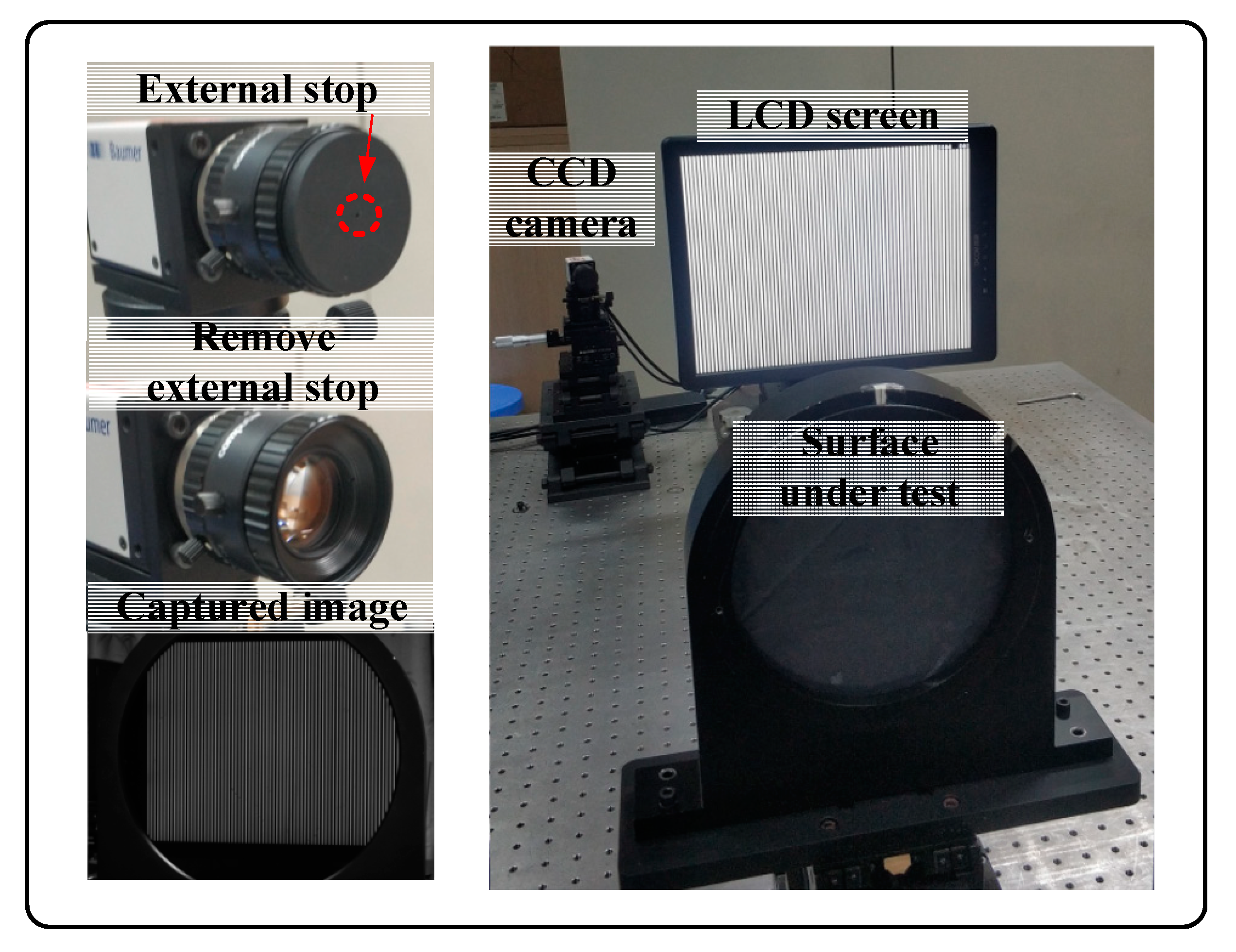
3.1. EPCM
- (a)
- The global coordinate system O-XYZ is established with point as the origin. Then, point and distance between the camera and the external stop in the z direction are determined;
- (b)
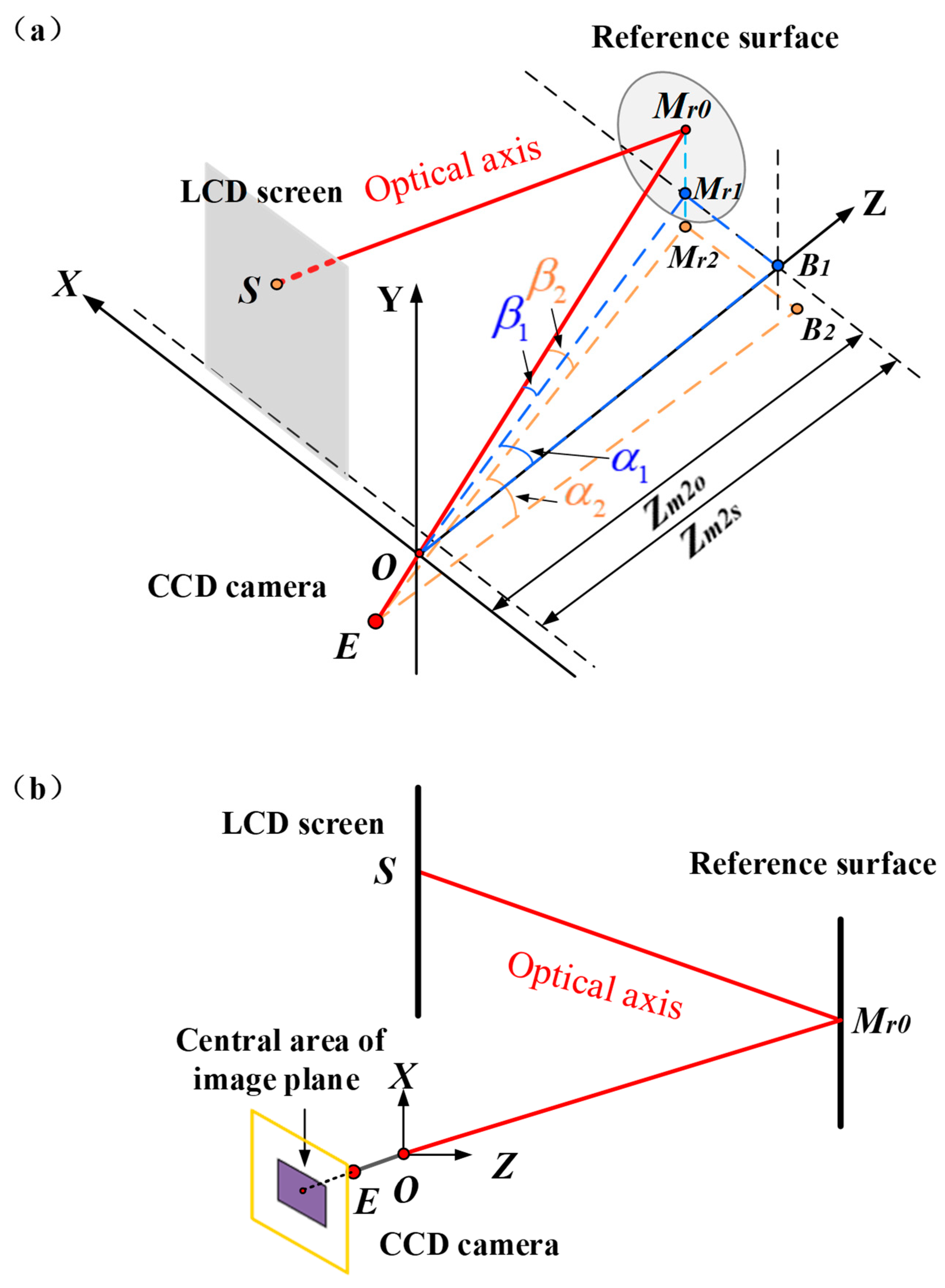
- The fringe pattern on the screen is reflected off the reference surface and captured by a camera equipped with an external stop. The screen coordinates corresponding to the central area of the image plane are calculated using the phase-shifting algorithm. The central area of the image plane with 2 M × 2 M pixels (M is a positive integer) is shown in Figure 1b. We calculate and obtain the coordinates of the reflection points of the reference surface using Equation (2); the coordinates of point can be obtained by the average of the reflection points corresponding to the central area of the image;
- (c)
- The distance between point and point can be measured in the experiment. The coordinates of point can be obtained by Equations (3) and (4) in the global coordinates;
- (d)
- The points of the reference surface are used as the initial values of the reflection points;
- (e)
- The slope is calculated using Equation (1) and the reconstruction height w from the slope. It is output after the height is less than the threshold;
- (f)
- The surface shape is reconstructed.
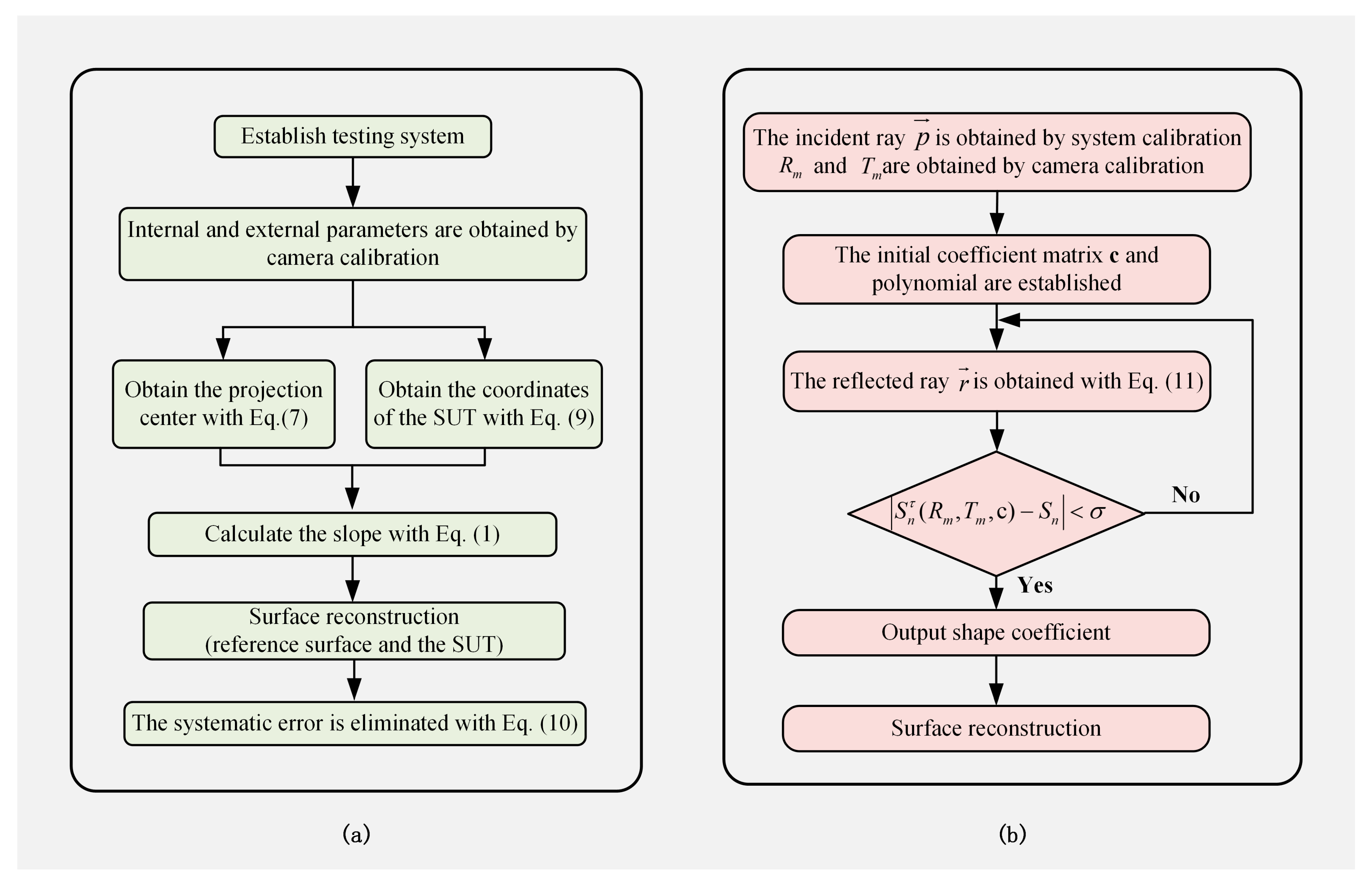
3.2. PM
- (a)
- The test system is established. It is worth noting that the last pose of the checkerboard plane is located at an identical position to the SUT, and it makes the local coordinate system on the last checkerboard parallel to each axis of the global coordinate system;
- (b)
- The rotation matrix R and translation vector T are obtained by camera calibration;
- (c)
- The projection center is obtained with Equation (7), and the coordinates of the SUT are calculated with Equation (9);
- (d)
- The slope is calculated with Equation (1), and the surface shape of the reference surface and the SUT are reconstructed;
- (e)
- The systematic error is eliminated with Equation (10).
3.3. MPMD
- (a)
- The incident ray is calibrated using the system calibration. The pose of the screen relative to the camera (, ) can be obtained through the pre-calibration procedure;
- (b)
- The initial coefficient matrix c and Zernike polynomial are used to represent the surface shape of the SUT;
- (c)
- The incident ray is reflected from the SUT to the screen. The reflected ray can be calculated with Equation (5), and the intersection on the screen is obtained;
- (d)
- The coefficient vector c and pose of the screen (, ) are optimized by minimizing the differences between the re-projection and the measurement S of the screen among the N pairs of correspondence in the least squares sense;
- (e)
- Output the shape coefficient and reconstruct the surface shape.
4. Accuracy Analysis
5. Experiment Results
5.1. Comparison of Camera Calibration
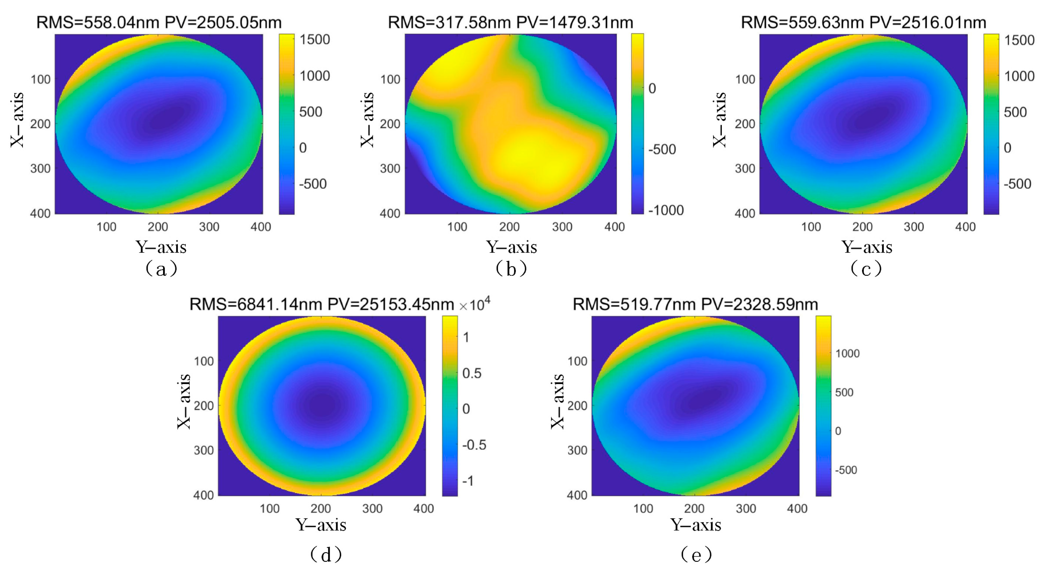
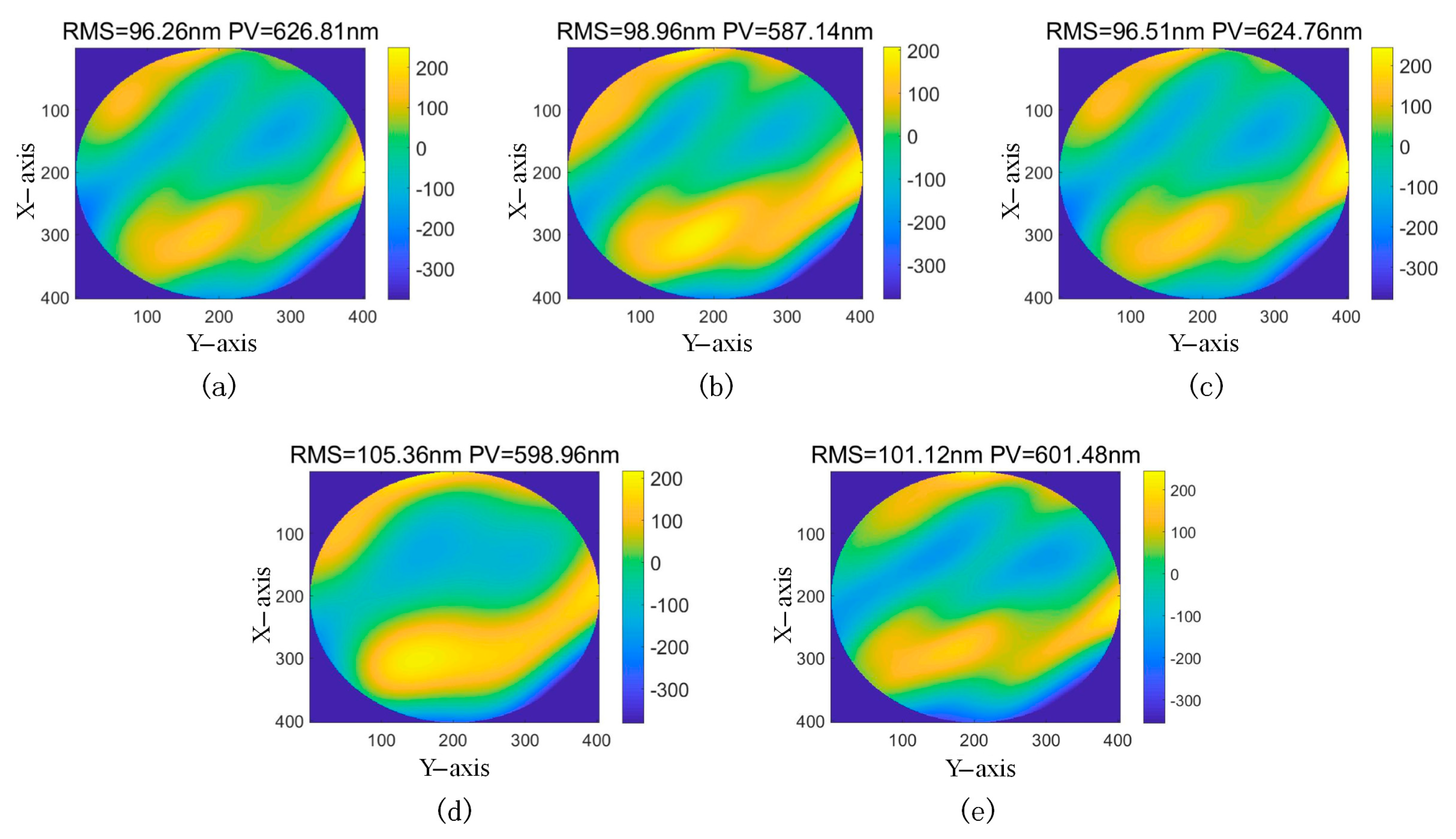
5.2. Comparison of Measurement Accuracy
6. Discussion and Conclusions
Author Contributions
Funding
Institutional Review Board Statement
Informed Consent Statement
Data Availability Statement
Conflicts of Interest
Appendix A
References
- Markus, M.C.; Knauer, J.; Hausler, G. Phase measuring deflectometry: A new approach to measure specular free-form surfaces. SPIE Photonics Eur. 2004, 5457, 366–376. [Google Scholar]
- Huang, L.; Idir, M.; Zuo, C.; Asundi, A. Review of phase measuring deflectometry. Opt. Lasers Eng. 2018, 107, 247–257. [Google Scholar] [CrossRef]
- Zhang, Z.; Wang, Y.; Huang, S.; Liu, Y.; Chang, C.; Gao, F.; Jiang, X. Three-dimensional shape measurements of specular objects using phase-measuring deflectometry. Sensors. 2017, 17, 2835. [Google Scholar] [CrossRef] [PubMed] [Green Version]
- Su, P.; Parks, R.E.; Wang, L.R.; Angel, R.P.; Burge, J.H. Software configurable optical test system: A computerized reverse Hartmann test. Appl. Opt. 2010, 49, 4404–4412. [Google Scholar] [CrossRef]
- Su, P.; Khreishi, M.; Su, T.Q. Aspheric and freeform surfaces metrology with software configurable optical test system: A computerized reverse Hartmann test. Opt. Eng. 2014, 53, 031305. [Google Scholar]
- Wang, R.Y.; Li, D.H.; Li, L.; Xu, K.Y.; Tang, L.; Chen, P.Y.; Wang, Q.H. Surface shape measurement of transparent planar elements with phase measuring deflectometry. Opt. Eng. 2018, 57, 104104. [Google Scholar] [CrossRef]
- Huang, L.; Xue, J.P.; Gao, B. Modal phase measuring deflectometry. Opt. Express 2016, 24, 24649–24664. [Google Scholar]
- Xu, Y.; Gao, F.; Jiang, X. A brief review of the technological advancements of phase measuring deflectometry. PhotoniX 2020, 1, 1–10. [Google Scholar] [CrossRef]
- Chen, P.Y.; Li, D.H.; Wang, Q.H.; Li, L.; Xu, K.Y.; Zhao, J.G.; Wang, R.Y. A method of sub-aperture slope stitching for testing flat element based on phase measuring deflectometry. Opt. Laser. Eng. 2018, 110, 394–400. [Google Scholar] [CrossRef]
- Kewei, E.; Li, D.H.; Yang, L.J.; Guo, G.R.; Li, M.Y.; Wang, X.M.; Zhang, T.; Xiong, Z. Novel method for high accuracy figure measurement of optical flat. Opt. Laser. Eng. 2017, 88, 162–166. [Google Scholar]
- Huang, R.; Su, P.; Burge, J.H.; Idir, M. X-ray mirror metrology using SCOTS/deflectometry. Proc. SPIE 2013, 8848, 88480G. [Google Scholar]
- Huang, R.; Su, P.; Burge, J.H.; Huang, L.; Idir, M. High-accuracy aspheric X-ray mirror metrology using Software Configurable Optical Test System/deflectometry. Opt. Eng. 2015, 54, 84103. [Google Scholar] [CrossRef]
- Luhmann, T. Close range photogrammetry for industrial applications. ISPRS J. Photogramm. Remote Sens. 2010, 65, 558–569. [Google Scholar]
- Sun, T.; Xing, F.; You, Z. Optical system error analysis and calibration method of high-accuracy star trackers. Sensors 2013, 13, 4598–4623. [Google Scholar] [CrossRef] [Green Version]
- Xiao, Y.; Su, X.; Chen, W. Flexible geometrical calibration for fringe-reflection 3D measurement. Opt. Lett. 2012, 37, 620–622. [Google Scholar] [CrossRef] [PubMed]
- Zhang, Z. A Flexible New Technique for Camera Calibration. IEEE Trans. Pattern Anal. Mach. Intell. 2000, 22, 1330–1334. [Google Scholar] [CrossRef] [Green Version]
- Hou, Y.; Su, X.; Chen, W. Alignment Method of an Axis Based on Camera Calibration in a Rotating Optical Measurement System. Appl. Sci. 2020, 10, 6962. [Google Scholar] [CrossRef]
- Sasián, J. Introduction to Aberrations in Optical Imaging Systems; Cambridge University Press: Cambridge, UK, 2011. [Google Scholar]
- Gennery, D.B. Generalized Camera Calibration Including Fish-Eye Lenses. Int. J. Comput. Vis. 2006, 68, 239–266. [Google Scholar] [CrossRef]
- Kumar, A.; Ahuja, N. Generalized Pupil-centric Imaging and Analytical Calibration for a Non-frontal Camera. Comput. Vis. Pattern Recognit. IEEE 2014, 3970–3977. [Google Scholar]
- Kumar, A.; Ahuja, N. On the Equivalence of Moving Entrance Pupil and Radial Distortion for Camera Calibration. In Proceedings of the International Conference on Computer Vision (ICCV), Santiago, Chile, 7–13 December 2015. [Google Scholar]
- Li, D.H.; E, K.W.; Li, M.Y. Study on the surface shape measurement of planar element based on slope sensor method. Acta Optica Sin. 2014, 34, 192–199. [Google Scholar]
- Zuo, C.; Feng, S.; Huang, L. Phase shifting algorithms for fringe projection profilometry: A review. Opt. Lasers Eng. 2018, 109, 23–59. [Google Scholar] [CrossRef]
- Wang, Z.; Han, B. Advanced iterative algorithm for phase extraction of randomly phase-shifted interferograms. Opt. Lett. 2004, 29, 1671–1673. [Google Scholar] [CrossRef] [PubMed]
- Zhao, C.; Burge, J.H. Orthonormal vector polynomials in a unit circle, part I: Basis set derived from gradients of Zernike polynomials. Opt. Express 2007, 15, 18014–18024. [Google Scholar]
- Zhao, C.; Burge, J.H. Orthonormal vector polynomials in a unit circle, part II: Completing the basis set. Opt. Express 2008, 16, 6586–6591. [Google Scholar] [CrossRef]
- Noll, R.J. Zernike polynomials and atmospheric turbulence. J. Opt. Soc. Am. 1976, 66, 207–211. [Google Scholar]
- Wang, R.Y.; Li, D.H.; Zhang, X.W. Systematic error control for deflectometry with iterative reconstruction. Measurement 2020, 168, 108393. [Google Scholar] [CrossRef]
- Bouguet, J.Y. Camera Calibration Toolbox for Matlab. Available online: http://www.vision.caltech.edu/bouguetj/calib_doc/S (accessed on 14 October 2015).
- Korsch, D.; Hunter, W.R. Reflective optics; Academic Press: Cambridge, MA, USA, 1991. [Google Scholar]


| Zernike Terms/Degree of Freedom | Z4 | Z5 | Z6 | Z7 | Z8 | Z9 | Z10 | Z11 | RSS | |
|---|---|---|---|---|---|---|---|---|---|---|
| The error of 1 mm is artificially introduced, respectively | 20.92 | −0.01 | 9.75 | 0.00 | 2.27 | 0.00 | −0.03 | −0.01 | 23.19 | |
| −0.11 | 9.91 | 0.05 | 2.32 | 0.00 | −0.03 | 0.00 | 0.00 | 10.18 | ||
| 160.06 | 0.00 | −1.73 | 0.00 | −0.54 | −1.66 | 0.00 | −0.04 | 160.08 | ||
| −42.34 | 0.03 | −19.74 | 0.00 | −4.58 | 0.00 | 0.06 | 0.02 | 46.93 | ||
| 0.06 | −19.98 | −0.03 | −4.68 | 0.00 | 0.05 | 0.00 | 0.00 | 20.52 | ||
| −2.67 | 0.00 | 0.03 | 0.00 | 0.00 | 0.00 | 0.00 | 0.00 | 2.67 | ||
| 21.43 | −0.01 | 9.99 | 0.00 | 2.30 | 0.00 | −0.03 | −0.01 | 23.76 | ||
| 0.07 | 10.24 | −0.04 | 2.40 | 0.00 | −0.03 | 0.00 | 0.00 | 10.52 | ||
| −162.73 | 0.00 | 1.75 | 0.00 | 0.55 | 0.00 | 0.00 | 0.05 | 162.74 | ||
| The error of 1 mrad is artificially introduced, respectively | Screen tilt x | −0.12 | 0.00 | 0.18 | 0.00 | 0.00 | 0.00 | 0.00 | 0.00 | 0.22 |
| Screen tilt y | −0.12 | 0.00 | −0.17 | 0.00 | 0.00 | 0.00 | 0.00 | 0.00 | 0.21 | |
| Screen tilt z | −0.10 | 352.02 | −0.17 | −0.52 | 0.00 | −0.42 | 0.00 | 0.00 | 352.02 | |
| flat tilt x | 0.12 | 0.00 | −0.18 | 0.00 | 0.00 | 0.00 | 0.00 | 0.00 | 0.22 | |
| flat tilt y | 0.12 | 0.00 | 0.17 | 0.00 | 0.00 | 0.00 | 0.00 | 0.00 | 0.21 | |
| RSS | 234.09 | 352.87 | 24.31 | 5.77 | 5.66 | 1.71 | 0.07 | 0.07 | - | |
| Methods/Coordinates | |||
|---|---|---|---|
| EPCM | 344.073 | 162.974 | −17.021 |
| PM | 338.571 | 162.928 | −21.154 |
| MPMD | 339.900 | 162.334 | −17.994 |
| Experiments/Methods | EPCM | PM with Systematic Errors | PM after Eliminating Systematic Errors | MPMD | Interferometer | ||||||
|---|---|---|---|---|---|---|---|---|---|---|---|
| RMS | PV | RMS | PV | RMS | PV | RMS | PV | RMS | PV | ||
| 1 | Removing the first 3 terms | 558.04 | 2505.05 | 317.58 | 1479.31 | 559.63 | 2516.01 | 6841.14 | 15,153.45 | 519.77 | 2328.59 |
| Removing the first 6 terms | 96.26 | 626.81 | 98.96 | 587.14 | 96.51 | 624.76 | 105.36 | 598.96 | 101.12 | 601.48 | |
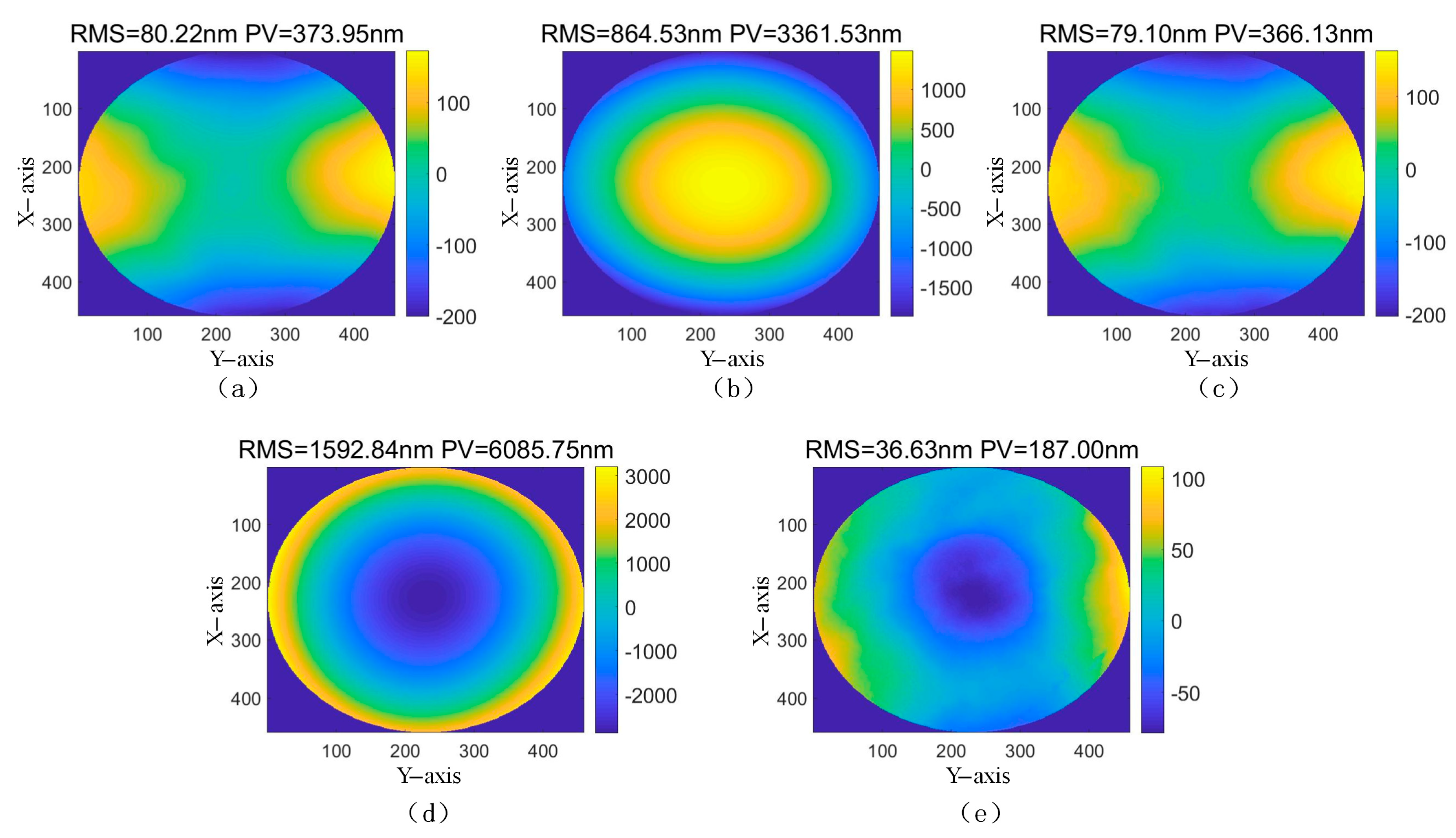
| 2 | Removing the first 3 terms | 80.22 | 373.95 | 864.53 | 3361.53 | 79.10 | 366.13 | 1592.84 | 6085.75 | 36.63 | 187.00 |
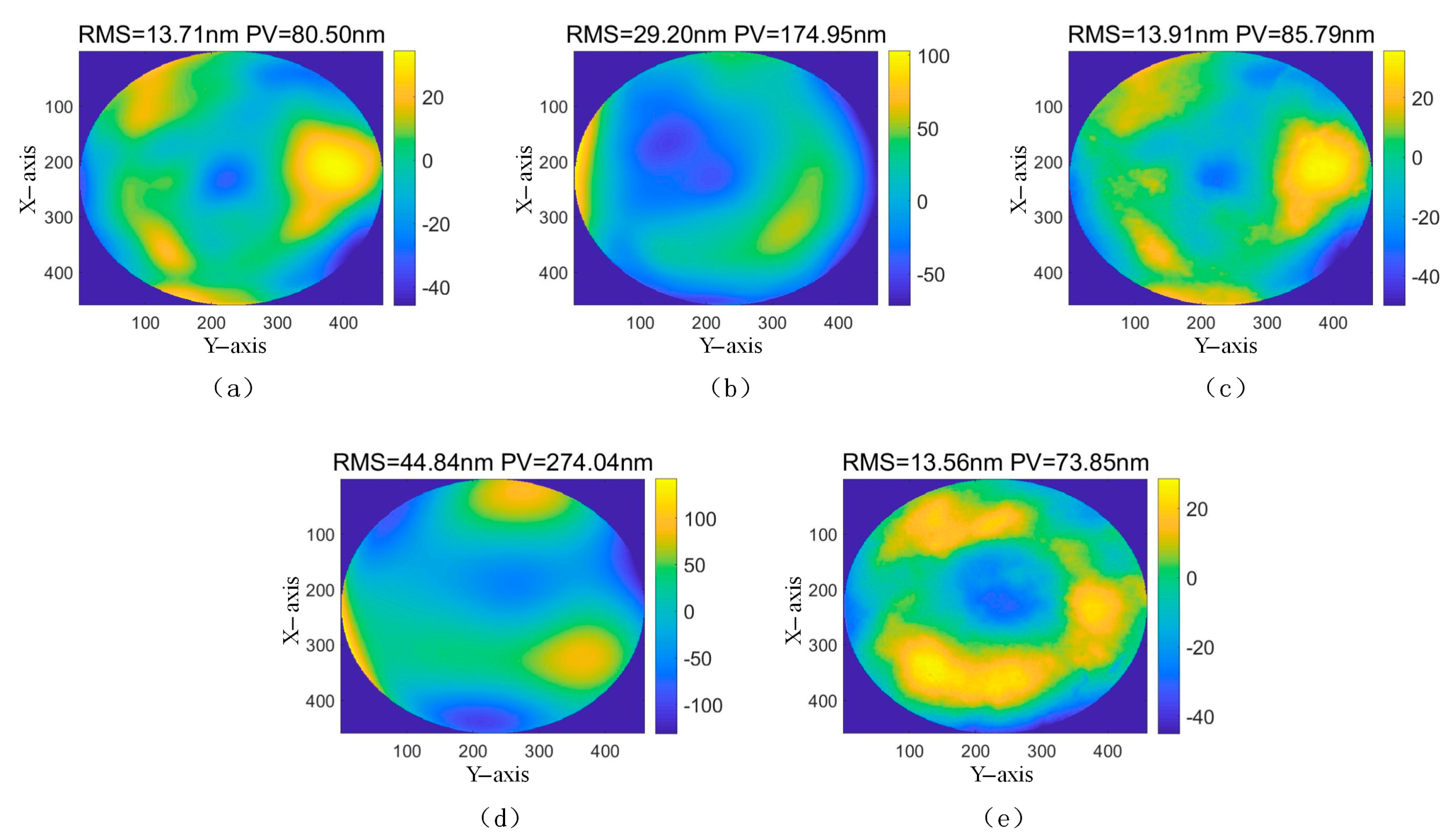
| Removing the first 6 terms | 13.71 | 80.50 | 29.20 | 174.95 | 13.91 | 85.79 | 44.84 | 274.04 | 13.56 | 73.85 | |
Publisher’s Note: MDPI stays neutral with regard to jurisdictional claims in published maps and institutional affiliations. |
© 2021 by the authors. Licensee MDPI, Basel, Switzerland. This article is an open access article distributed under the terms and conditions of the Creative Commons Attribution (CC BY) license (https://creativecommons.org/licenses/by/4.0/).
Share and Cite
Ge, R.; Li, D.; Zhang, X.; Wang, R.; Zheng, W.; Li, X.; Zhao, W. Comparison of Camera Calibration and Measurement Accuracy Techniques for Phase Measuring Deflectometry. Appl. Sci. 2021, 11, 10300. https://doi.org/10.3390/app112110300
Ge R, Li D, Zhang X, Wang R, Zheng W, Li X, Zhao W. Comparison of Camera Calibration and Measurement Accuracy Techniques for Phase Measuring Deflectometry. Applied Sciences. 2021; 11(21):10300. https://doi.org/10.3390/app112110300
Chicago/Turabian StyleGe, Renhao, Dahai Li, Xinwei Zhang, Ruiyang Wang, Wanxing Zheng, Xiaowei Li, and Wuxiang Zhao. 2021. "Comparison of Camera Calibration and Measurement Accuracy Techniques for Phase Measuring Deflectometry" Applied Sciences 11, no. 21: 10300. https://doi.org/10.3390/app112110300