Abstract
With the development of the social economy and the improvement of the consumption concept, a new business model combining offline and online has been promoted. The warehousing system is one of the important links of commodity production and circulation, which involves storage, sorting, and distribution. It has a significant impact on the operation cost and the efficiency of the whole logistics system. The progress of robot technology, the Internet of things, and artificial intelligence technology promotes the automation and intelligence of storage systems. The Robotic Mobile Fulfillment Systems (RMFS), which takes the automatic guided vehicles (AGVs) as the way of handling and picking, greatly improves the space utilization, operation efficiency, and flexibility of the system. This paper studies the RMFS with fixed shelves and establishes the performance evaluation model of the picking system considering the AGVs congestion by establishing the queuing network. The effectiveness of the model is verified by simulation, and the optimization of system parameter configuration is further discussed according to the experimental data.
1. Introduction
With the development of Industry 4.0 and the rise of e-commerce, the level of intelligence and modernization in logistics has been significantly improved. The continuous upgrading of consumption concept has promoted the integration of online and offline retail, and a new retail business model has emerged, as the times require. The storage system is a key step in logistics, involving commodity storage, distribution, and information circulation, which has a significant impact on the operation cost and operational efficiency of the whole logistics system [1].
The Robotic Mobile Fulfillment Systems (RMFS) adopts automatic guided vehicles (AGV) to carry goods, which saves the walking time of the picker and greatly improves the order picking efficiency of the system [2]. The storage and picking equipment of the system is deployed on the ground with high flexibility and scalability, so the system layout and configuration adjustment are convenient. In addition, the picking operation is carried out on the ground, the human-computer interaction is convenient, and the system operation flexibility is high [3].
The operation strategy of the RMFS incorporates rules and methods that should be followed in the picking process. Therefore, the operation strategy of the system will directly affect the operational performance of the system. The main function of RMFS is to pick customers’ orders. Improving its operation performance can directly improve the order delivery efficiency and improve customers’ shopping experience. Therefore, many researchers have engaged in the optimization of the RMFS operation strategy [4].
In the RMFS, AGVs and pickers are used to complete order picking, so there are order picking tasks and resource allocation and scheduling problems. Zou et al. [5] proposed an order allocation strategy based on the picking speed of the picking table and designed a near neighborhood search algorithm to find the near-optimal allocation strategy. Xie et al. [6] focused on the allocation of order tasks to the picking station and the allocation of shelves to the picking station, built a centralized optimization model, and proposed a strategy where orders can be split and allocated to different picking stations to minimize the number of picking times. Dou et al. [7] considered a method to improve the operation efficiency of the system that combined a task allocation strategy based on a genetic algorithm (GA) and a path planning strategy based on reinforcement learning (RL). Zhang et al. [8] modeled an AGV allocation problem in the order-picking task as a resource-constrained scheduling problem, and designed a genetic algorithm to solve it. The experimental results showed that the task allocation strategy proposed in this study was more effective than the current practical task allocation method based on general rules. Merschformann [9] considered the order task allocation, shelf selection, and shelf storage allocation and evaluated several system operation performance indicators. The research showed that the order task allocation strategy had the greatest impact on the order picking throughput of the system. Roy et al. [10] considered the allocation of AGVs to each storage area when the system had multiple picking areas. In this study, a strategy that allocated the AGVs to the area with relatively minimum order picking throughput was proposed, which could greatly improve the system order throughput compared with a random allocation strategy. Zhe et al. [11] evaluated the performance of the RMFS by establishing an open-loop queuing network model. The model was used for numerical analysis and experiments to optimize the number of the AGVs, the number of the picking stations, and the speed of the AGVs. Lienert et al. [12] established a simulation model for the RMFS to predict system operation performance. This study analyzed the impact of different AGV numbers on order picking throughput of the system. Zi et al. [13] established an M/M/s queueing model to estimate the throughput of the AGV sorting system. The influence of some system parameters on throughput was analyzed through numerical experiments. Koo et al. [14] presented a queueing model to estimate the part waiting times in a manufacturing system that included AGVs. Cui et al. [15] designed a Flexsim simulation model of AGVS in a manufacturing workshop, which could be used to study the shortest moving path and the lowest cost. Chen et al. [16] explore the problem of workstation arrangement in a production system. The combination of an open queuing network model and simulated annealing found a good solution to this problem. Azenha et al. [17] described an artificial neural network (ANN) approach for AGV positioning in an indoors quasi-structured environment.
In robots research, Kemény et al. [18] provided an overview of multi-agent robot systems relying on distributed artificial intelligence. Zacharaki et al. [19] discussed the safety problem and the risk assessment techniques in the field of human-robot interaction. Pratama et al. [20] presented a fault detection algorithm to analyze the sensors and motors of AGVs based on multiple positioning modules. Witczak et al. [21] concentrated on a strategy based on a fault-tolerant control framework and improved the sustainability and flexibility of the warehouse AGV system. Wang and Liu et al. [22,23] studied the application of robots in the Shuttle Warehousing System.
Based on the structural comparison of the fixed shelves AGV system, this paper has selected the most common fixed shelves system as the research object. We construct a semi open-loop queuing network model to evaluate the parameters of the system considering congestion factors such as the throughput and the congestion delay time, and finally verify the effectiveness and accuracy of the model through simulation and experimental analysis.
2. System Introduction and Scheduling Rules
2.1. Overview of the AGV Picking System
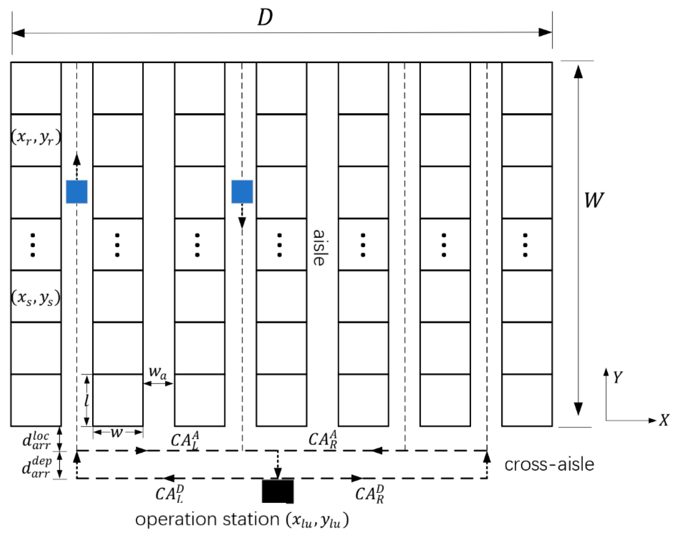
In the fixed shelves AGV picking system, the operation mode is divided into a single instruction mode and double instruction mode. Single instruction mode means that only a single storage task or a retrieval task is completed in each operation, while double instruction mode means that one storage task and one retrieval task are completed at the same time. In the system studied in this paper, the double instruction mode was adopted; that is, each task execution process included a storage task operation and a retrieval task operation. In order to model the system, we first study its operation process and decompose each subdivision action of the operation process. The whole operation process can be divided into three stages. The following Figure 1 describes each stage of the operation process.
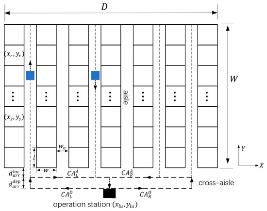
Figure 1.
The AGV picking system.
The first stage is to leave the operation station by the cross-aisle, which means to select the left cross-aisle or the right cross-aisle after taking material from the operation station to enter the shelves system.
The second stage is the process in the aisle; that is, entering the aisle through the connection called and between the aisle and the cross-aisle, storage of the material in an empty location, then arriving at the designated location to take out the materials and returning to the aisle exit. This stage is the main operation link.
The third stage is to arrive across the cross-aisle; that is, to enter the left cross-aisle or right cross-aisle from the aisle port through the connecting section and , the link from the shelves system to the operation station.
After completing the above three stages of operation, the AGVs will arrive at the operation station, complete the material interaction through manual or equipment docking, and end the operation process.
2.2. Modeling and Symbol Definition
In order to achieve effective analysis, this paper makes the following assumptions.
- Only one operation platform is considered.
- The AGVs have different running speeds in the aisle, cross-aisle, and connecting sections. The speed in the aisle is faster, and other sections are driven at low speed, which is in line with the actual scene of AGV.
- Task instruction includes picking tasks and replenishment tasks. This paper only considers picking tasks. In addition, it is assumed that the storage area always contains enough materials to meet each entry task of the system.
- The time interval of task arrival obeys exponential distribution.
- The service of AGV in the cross-aisle and the operation station follows the principle of first come, first served (FCFS).
- The processing time at the operation station obeys the general distribution.
- Tasks are always assigned randomly, which means that if we partition the storage area, the location of each area is random. If there is no partition, the entire area follows random rules.
- AGV returns to the buffer position of the operation station after each task is completed, which is used as the parking space for the next task.
- The cross-aisle only allows one-way traffic, and the traffic congestion in the cross-aisle is not considered.
The main symbols used in this paper and their meanings are listed in Table 1.

Table 1.
Main system parameters and their meanings.
2.3. Congestion Factors and Scheduling Rules
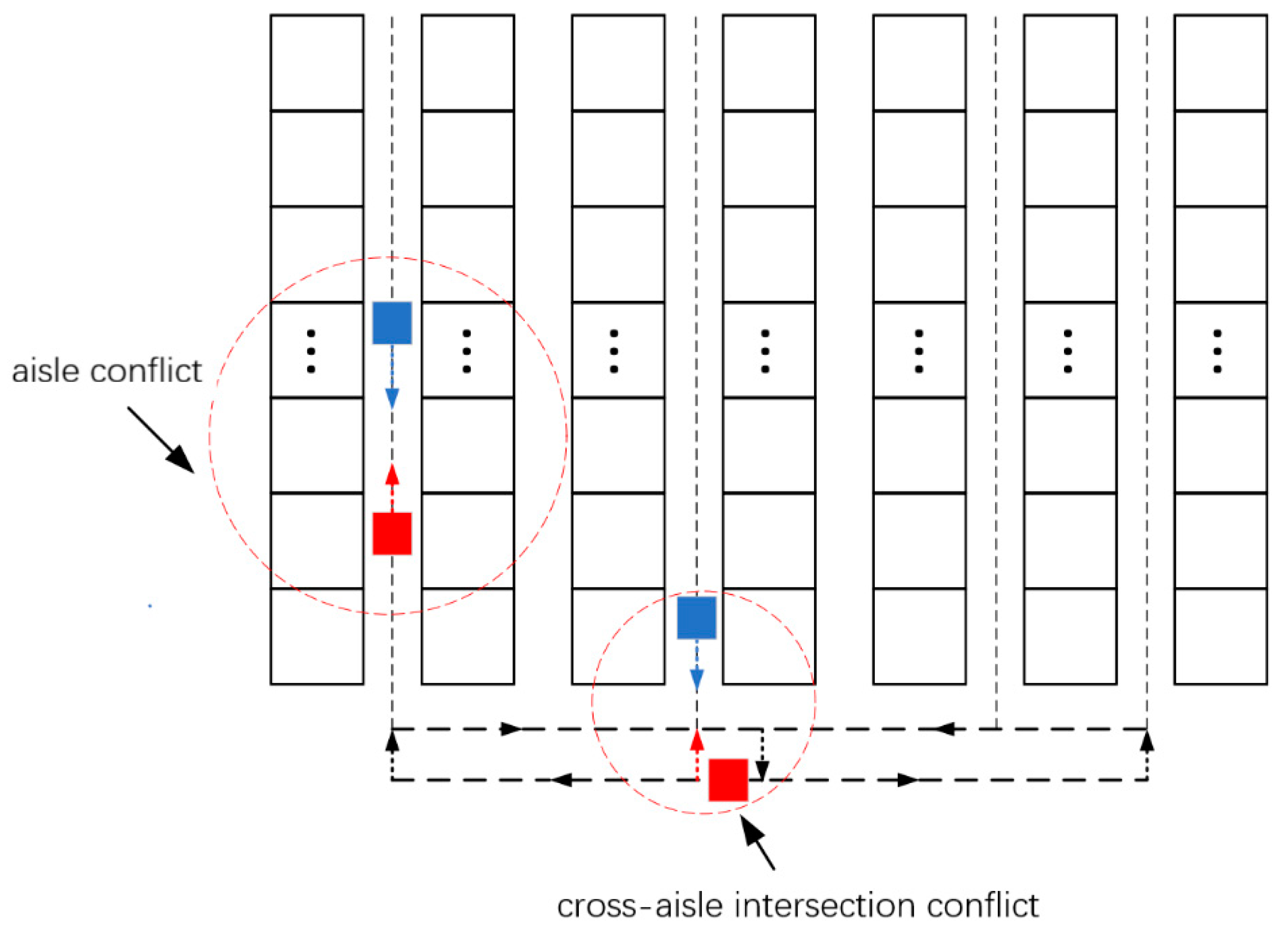
There will be vehicle congestion in the RMFS with fixed shelves; that is, multiple AGVs occupy the same space resource at the same time, resulting in vehicle delay. In this system, the cross-aisle is a one-way driving path (the departure and arrival directions belong to two paths), and the AGV driving on the same path is in the same direction with the constant speed, so the cross-aisle conflict is not considered. Therefore, the congestion phenomenon in the system can be divided into two kinds of routing conflicts, namely, aisle conflict and cross-aisle intersection conflict. The specific congestion situation is shown in Figure 2.
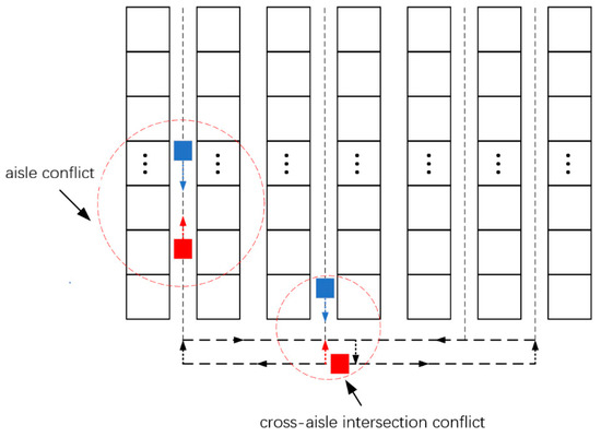
Figure 2.
Schematic of the congestion.
In the aisle, the path setting is two-way driving. Therefore, when an AGV is already in the aisle and another AGV tries to enter the aisle, there is a conflict phenomenon. In the same way, when one AGV tries to leave the aisle to enter the cross-aisle and another AGV is driving or preparing to enter the aisle from the cross-aisle, the intersection conflict will occur. In order to solve this conflict, the rule called LCFS-PR (last come, first serve preemptive resume) is proposed to be used in the aisle. When the service rule is used, the priority of the existing AGV in the aisle is lower than that of the later arriving AGV. That is, when the latter arrival AGV tries to request access to the aisle, the AGV working in the same aisle will drive to the end port of the aisle, and then it will continue to work after the latter arrival AGV finishes the operation. By considering the use of the service rules in the modeling process, the focus of this paper is to study the impact of congestion factors on system performance.
When the AGVs conflict in the intersection of the cross-aisle and the aisle, the system will appear as a congestion phenomenon. In order to solve this problem, a rule is formulated, that is, after each operation in the aisle, the AGV leaves the aisle immediately and waits to enter the cross-aisle at the shelf port where the aisle connects with the cross-aisle.
3. Modeling and Solution
3.1. Semi-Open Loop Queuing Network Model (SOQN)
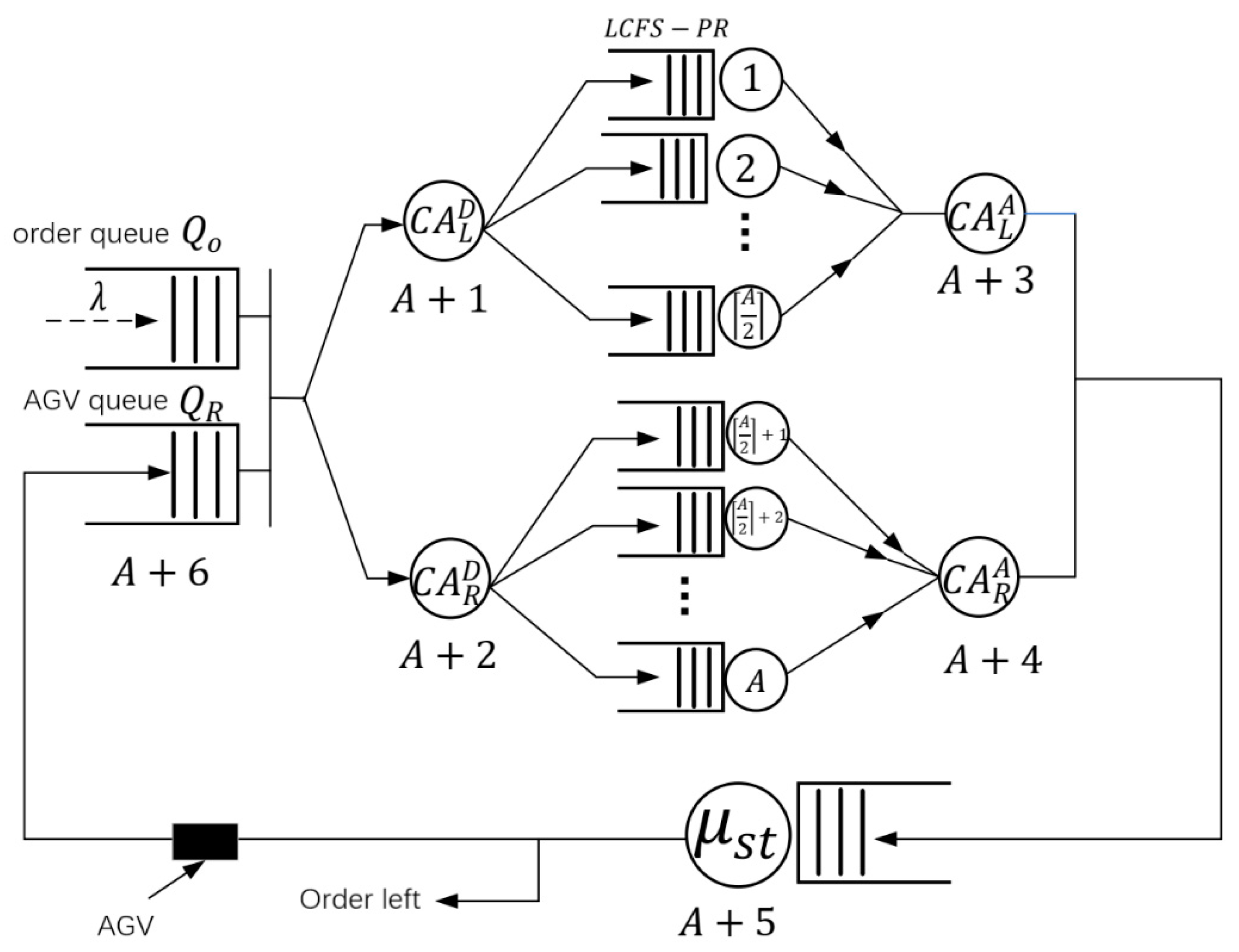
According to the system analysis and scheduling rules, the semi-open loop queuing network model of the AGV system can be established, as shown in Figure 3. In this model, the AGV in the warehouse is regarded as a secondary resource when it performs the task of loading and unloading. It is assumed that the AGV is running at a constant speed without considering the acceleration and deceleration process. The assignment strategy of the AGV is the random assignment; that is, any idle AGV can be assigned to any task as soon as possible. It is assumed that the arrival rate of the external task arrival system obeys Poisson distribution. The task service in the system follows the first come, first serve rule (FCFS). In this SOQN model, the number of service nodes is equal to , in which the aisle nodes are parallel service desks. Each aisle belongs to a node, evenly distributed on the left and right sides of the cross-aisle, each with nodes. So the network has aisle nodes. There are four cross-aisle nodes in the system. That is the left cross-aisle node and right cross-aisle node for leaving the station correspond to and in the network model respectively, and the left cross-aisle node and the right cross-aisle node for arriving the station correspond to and in the network, respectively. The station node is identified with , and the virtual synchronization service node used by the system to match AGV car and external task queue is identified with .
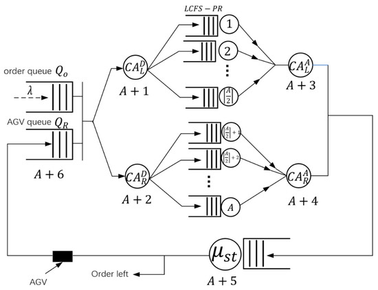
Figure 3.
Queuing network model of the AGV system.
When a task arrives in the system and enters the external order queue . The synchronous node finds an idle AGV in the AGV queue and matches it with a task. Then, the material is transported by AGV through one of the cross-aisle nodes to leave the station. It is equally possible for AGV to pass the left cross-aisle node or the right cross-aisle node and enter the aisle nodes on the left and right sides, and the probability is . The AGV then enters the designated aisle node to unload and load the next material and leaves the aisle node to return to the operation station to process the material through the cross-aisle nodes. After completion of the picking work, the released AGV re-enters the inner AGV queue to wait for the next assignment. In the selection of the aisles, the uniform distribution strategy is adopted, and the probability of choosing each aisle is equal to . That is to say, any AGV can be assigned to any task in any aisle equally.
This queueing network model has the characteristics of both closed network and open network, which is called semi-open queueing network model. Because the external tasks arrive at the system continuously and enter the external queue , it has the property of an open network. At the same time, because the number of AGV in the system is limited and they always exist in the system, any task arriving in the system needs to wait for the matching with the idle vehicles to carry out the execution process. So the network also has the property of a closed network. In order to ensure the steady-state of the queuing network model, the arrival rate of the task should be less than the maximum throughput calculated by the closed network system when there are vehicles in the system. That is, the number of tasks arriving at the system per hour should be less than the number of tasks that can be processed per hour when all AGVs are busy. The semi-open queueing network described above is a non-product form, so an approximate method is needed to solve the model [24]. Before solving, the service time expression of each node in the network is described.
3.2. Service Time Expression of Each Node
Firstly, to calculate the service rate of each service node, the service time of each node is needed. The service time expressions of aisle, cross-aisle, and operation station are given in turn.
3.2.1. The Service Rate and the Parameter Estimation in the Aisle
The service time of AGV in the aisle includes the whole running time after entering the aisle from the aisle port, selecting a location to store materials, and taking out materials from another location to return to the aisle port. Set is the running time in the aisle, is the time to store material, is the time to take out a material. In addition, the service time also includes the time from the cross-aisle to the aisle port. Therefore, the aisle service time expression is obtained.
In this expression, only is unknown, and its expected value needs to be estimated according to the storage strategy of the storage area. Next, we estimate the solution of under the random storage strategy and the classified storage strategy. Let is the location number of the storage shelf, is the location number of the rack, represents the running distance from the storage location to the pickup location and return to the starting aisle port.
It is set that there are material spaces on each floor of the aisle. Under the random storage strategy, The values of and are relatively independent. So the joint probability of and can be expressed as
Let , then the probability function of is expressed as
The first and second moments of can be expressed as
According to Formulas (2), (5) and (6), the first and second moments of the round trip distance can be obtained as
Therefore, both the time expectation of and the second moment of it can be obtained as
According to Formulas (1), (9) and (10), the expected service time and the second moment in the aisle can be obtained as
The aisle service rate, the variance of expected service time, and the variance coefficient of the square formula are as follows
3.2.2. The Service Rate in the Cross-Aisle
The process in the cross-aisle is simulated as an infinite capacity service station, and the running distance in each cross-aisle is expressed as
The service time and the service rate in the across-aisle are expressed as
3.2.3. The Service Rate of the Picking Station
The service rate of the picking station depends on the operation time of the picker or the picking equipment, which is usually constant. We set that the time for the picker to complete a task is , then the service rate of the picking station is expressed as
3.3. Solution
The SOQN model had no product-from solution, so the Decomposition Method was introduced to solve it. The whole SOQN was decomposed into two sub-networks, a closed network and open network, and the eigenvectors were solved, respectively. Then the queue length of each node was calculated, and the performance parameters of the whole system were analyzed.
Where , then represents the difference between the internal and external queues at the synchronization node. When is greater than 0, the number of external task queues is larger than that of the internal AGV queue; that is, the task needs to wait for idle AGV. When is less than 0, it means that the number of AGV in the queue is greater than the task; that is, AGV is waiting for the task of the external queue. The Decomposition Method is to decompose the semi-open queue network into two closed networks , and an open network . When equals 0, it has both open queueing network and closed queueing network characteristics.
3.3.1. Establishment and Solution of the Closed Queueing Network Model CQN1
A closed-loop queuing network model CQN1 was established, in which the synchronous nodes were regarded as exponential service stations. In this network, aisle nodes were LCFS-PR type service stations, and cross-aisle nodes were infinite capacity service stations. Idle AGVs queue up to wait for the task to arrive at the synchronization node . We set the task arrival system to obey the Poisson process, then the average service time of the synchronization node obeyed the parameter . The service rule was first come, first service (FCFS). The closed-loop queuing network had no product type solution according to the assumption of the model, and the Approximated Mean Value Analysis (AMVA) method was introduced to solve the problem. The marginal probability of each node in the network was . The conditional probability of the synchronous node with idle AGVs, could be derived from the following formula with the marginal probability .
Finally, the average conditional queue length of each node awere obtained.
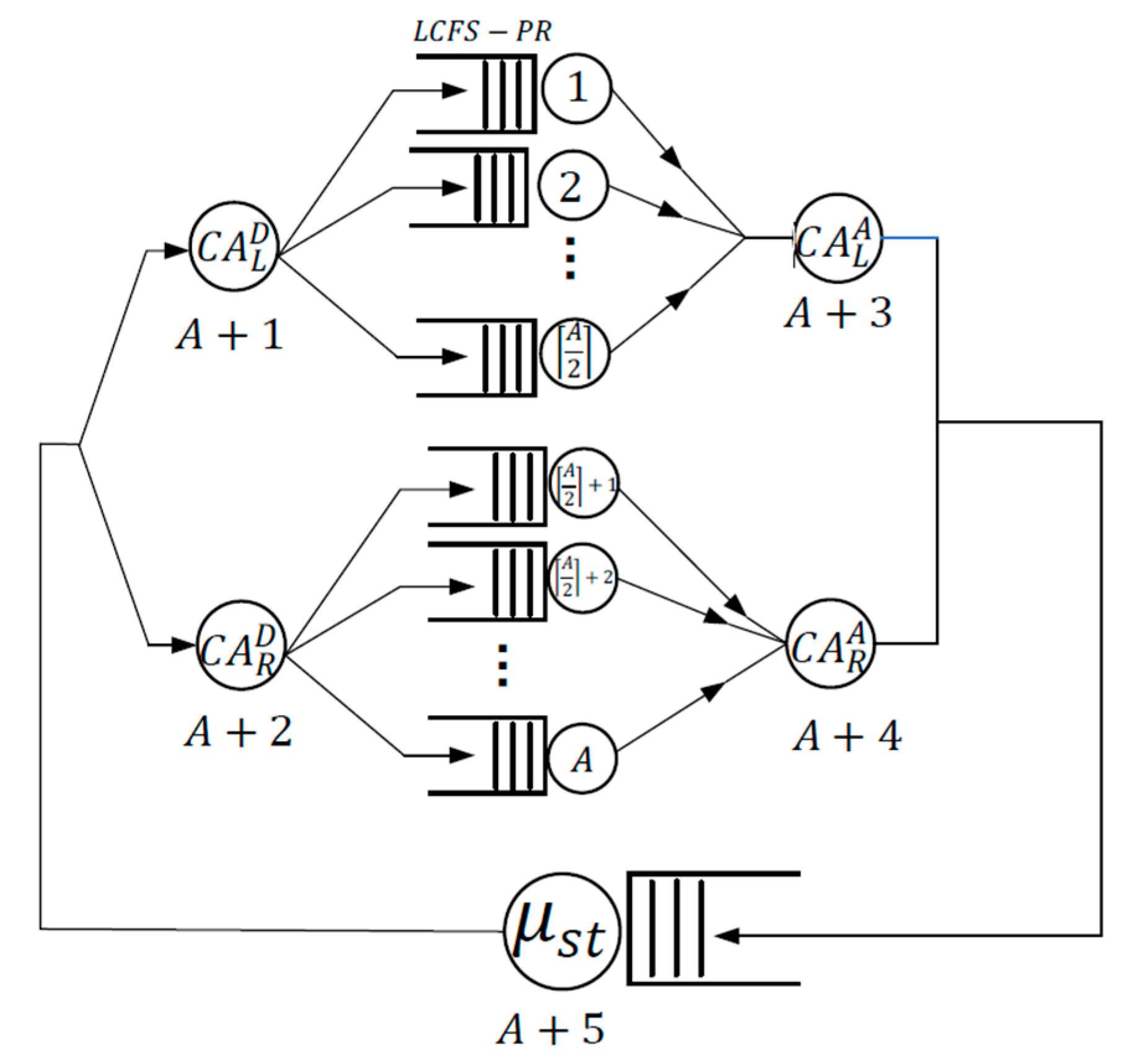
3.3.2. The Second Closed-Loop Queuing Network Model CQN2
The synchronous station node was removed from CQN1, and the second closed-loop queuing network model CQN2 was constructed. The difference between this closed-loop network and the closed-loop network CQN1 is established when y ≤ 0 is only at the synchronization node.
As shown in Figure 4, the synchronization node was removed from this network. When a task comes into the system, all vehicles were busy. Once an AGV became idle, it was assigned to a task immediately. This network simulates the scene of ; that is, there is no vehicle in the queue waiting for the task. There was still no product-form solution to the CQN2, so the AMVA method was introduced again to solve the network. Then the marginal probability of each node was obtained. Similarly, the average conditional queue length of each node was obtained.
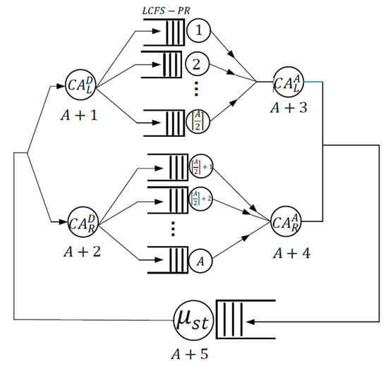
Figure 4.
Queuing network model CQN2.
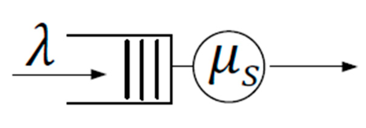
3.3.3. Establishing an Open-Loop Queuing Network OQN
When , the task is waiting for the idle AGV in the external queue. When the AGV is free, the arriving tasks are bound to it. The system can be analyzed as a single queuing system that follows a Poisson arrival parameter , as shown in Figure 5.
Figure 5.
Queuing network OQN.
The key to solving this queuing system was to decide the service time of the service station. We set that was the rate at which idle AGVs become executable. depends on the distribution of busy AGVs in the aisle and the cross-aisle; it is equal to the system throughput of CQN2. In order to accurately determine the service time distribution of task waiting vehicles, it was necessary to calculate the higher-order moment of service time of OQN and determine the type of queuing system. The calculation of the higher-order moment of OQN service time needed to analyze the customer departure process of CQN2 when all vehicles were busy. Specifically, the higher-order moments of each node in CQN2 needed to be calculated, and the results showed that each service time has a low variation. Therefore, we choose to approximate this OQN to an M/D/1 queue. Then, the average queue length and steady-state probability were obtained by Pollaczek–Khinchin and LS transformation equations, respectively. From this solution of the OQN, we could get the number of conditional queueing tasks waiting in the external queue .
3.3.4. Converged Network
Under the conditions of and , the above solution gives the steady-state probability distribution of the vehicle and task and in the network respectively. According to the law of total probability and the fact that the state conforms to the attributes of both open-loop and closed-loop networks, the above conditional probability was fused to obtain the unconditional probability distribution. Because state satisfies two conditions, the following formula was established:
In this formula, the probability and is unknown. They can be obtained by the following steps. First of all, we order is the utilization rate of the OQN system M/D/1, then the conditional probability Then use this variable to replace the above , the following formula can be obtained:
Further, because , the following formula can be obtained:
The unknowns and can be obtained by these two formulas. After we get and , the unconditional probability in the case of and can be obtained respectively by the following formula:
After the unconditional steady-state probability is solved, the key performance indexes are calculated based on it, including vehicle utilization, idle vehicle distribution, average waiting queue length, etc.
3.3.5. Performance Index Estimation
The solution of the SOQN model gives the average queue length of vehicles at node . The formula of is as follows:
The main performance index of the system is the utilization rate of the vehicle , task cycle time or throughput time , the average length of tasks waiting for service in external queue , the expected aisle blocking delay time . The number of idle vehicles in the internal queue can be obtained by calculating the average number of customers in the synchronization node.
The proportion of idle vehicles is expressed as . Then according to the Utilization Law, the utilization rate of the vehicle is expressed as . According to the Pollaczek–Khinchin average queue length equation of the M/D/1 queuing system, the average queue length of the external queue can be obtained. The external queue only exists when , that is, . The unconditional queue is obtained by multiplying the conditional value by the steady-state probability, the formula is as follows:
According to the average queue length and Little’s Law, the expected task cycle time can be obtained. Task cycle time includes two parts, one is the average waiting time of task matching idle vehicle, the other is the task execution time. Therefore, the task cycle time is expressed as the following formula:
The delay time due to blockage can be calculated by calculating the waiting time in the aisle. By using Little’s Law to calculate the running time of the vehicle in the aisle, the expected aisle blocking delay time can be obtained as follows:
After the delay time of aisle blockage and the cycle time of expected tasks are obtained, the ratio of the delay time of aisle blockage can be obtained, and the influence of delay factors on system performance can be analyzed. The ratio is . Then the accuracy of the solution and the influence of blocking delay factors on the system performance is analyzed through specific simulation and numerical experiments.
4. Simulation and Result Analysis
4.1. Simulation
The simulation model is used to verify the theoretical model. In order to ensure the validity and reliability of the model, different scene experiments are obtained by changing the system design parameters. In this paper, the discrete event simulation module of Matlab’s Simulink function was used to simulate the queuing network model.
The simulation model was built according to the process of the queuing network. The first was random task generation. The random arrival process was generated by an exponential function, which obeys the Poisson distribution. The generated task was bound to AGV through a resource acquisition device. If there was no idle AGV at that time, the task would wait in the external queue. Finally, after binding with the idle AGV, the task entered the shelves system to receive service.
The process of receiving service after entering the shelves system is as follows: First, enter the cross-aisle service, and choose the cross-aisle node on both sides with equal possibility. There is no waiting in this cross-aisle node because it is assumed that the cross-aisle node is an infinite capacity service node. Then the aisle node service is carried out. If there is already AGV working in the selected aisle, the AGV that are working in the aisle will enter the waiting queue. Later AGVs are served first, the queuing rule is Last In, First Out (LIFO). After the AGV completes the service in the aisle, it returns to the end port of the aisle and enters the cross-aisle service node again. Similar to the previous cross-aisle node service, it directly enters the cross-aisle service without waiting. Finally, the task with the AGV enters the queue of the picking station. If the picking station is free, the task will be served. If there are vehicles in operation, the task will wait in the queue. After completing the service, the AGV is released by the resource releaser. The task leaves the system, and the AGV returns to the resource pool to wait for matching the next task.
The parameters of each node can be calculated according to the service time calculation expression in Section 3.2 and the given warehouse layout design parameters. The system parameters used in the simulation model are in Table 2.
Table 2.
System setting parameters in simulation.
In order to fully verify the effectiveness and reliability of the theoretical model, we change the number of storage spaces , the aspect ratio of storage area and the task arrival rate of the system to generate multiple scenes. For each scenario, the simulation model first runs 100 h of warm-up time to eliminate the system error as far as possible and then runs 100 times for 1000 h to achieve no less than 95% confidence. The collected index includes the average tasks queue waiting length of the synchronization node , the AGV utilization , order throughput time , the average congestion delay time and the congestion time proportion .
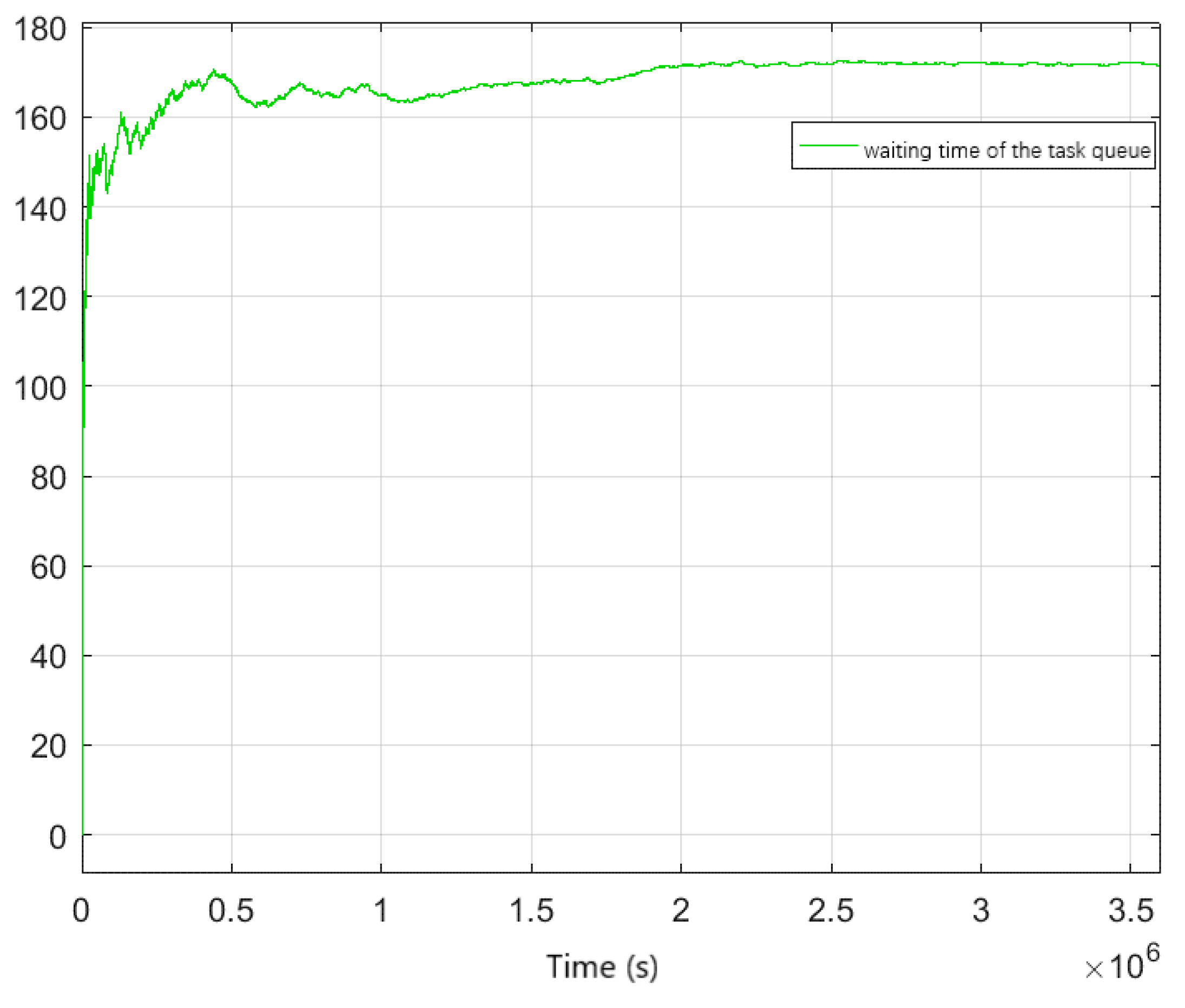
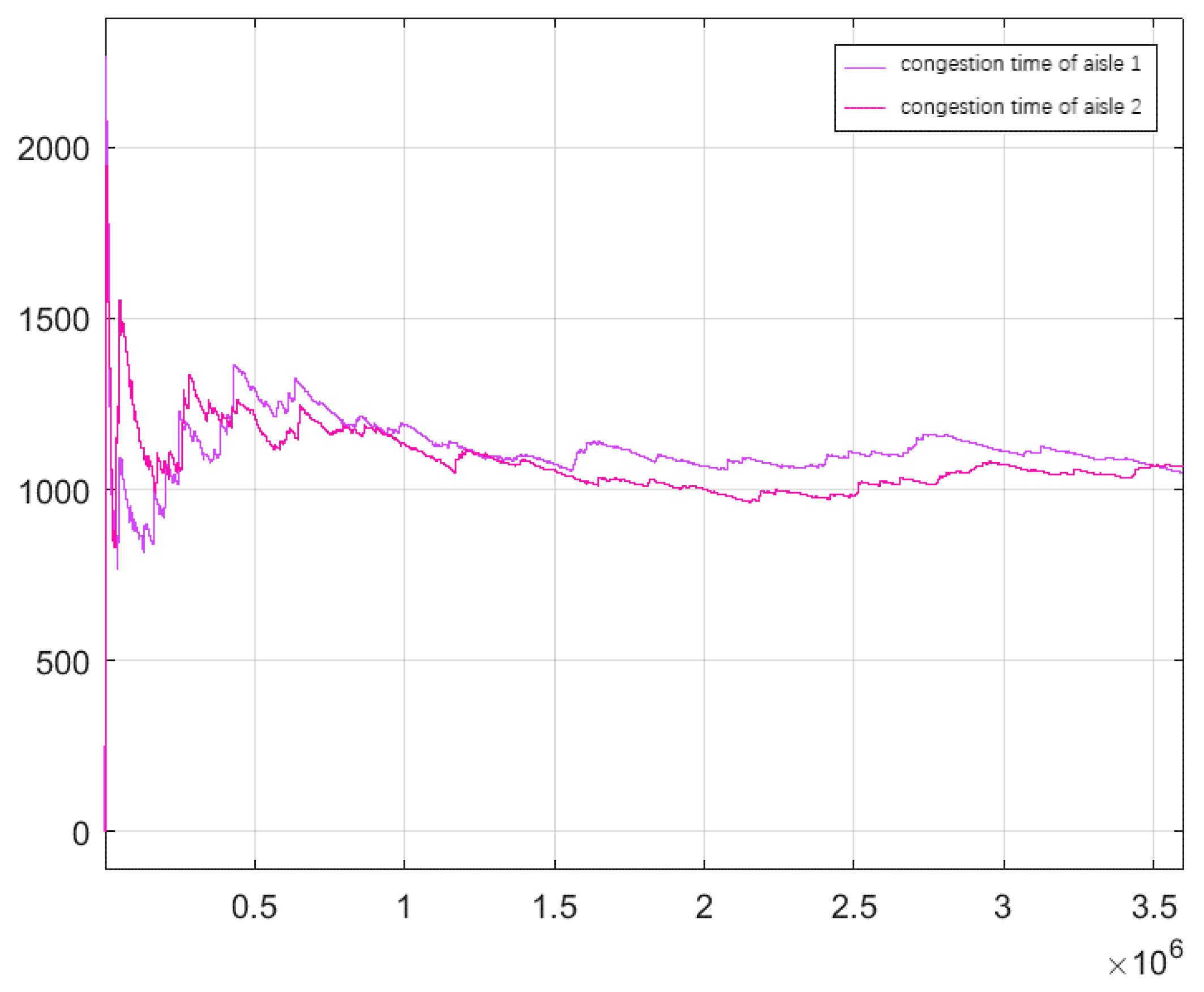
During the running of the simulation model, the waiting time index of the task is tracked. We draw the curve of the tracking result at the synchronous matching node, as shown in Figure 6 above. It can be seen from the trend of the curve in Figure 6 that the waiting time of the task queue in the first 100 h was oscillatory. After the system reached a stable state, the change of the delay time was very small. Similarly, we tracked the congestion time of any two aisles and drew a graph, as shown in Figure 7. The system vibrated severely in the first 150 h, and then the fluctuation of the congestion time curve became very small as the system gradually ran to a stable state. We took the average delay time of all aisles as the simulation result of the congestion time to reduce the error.
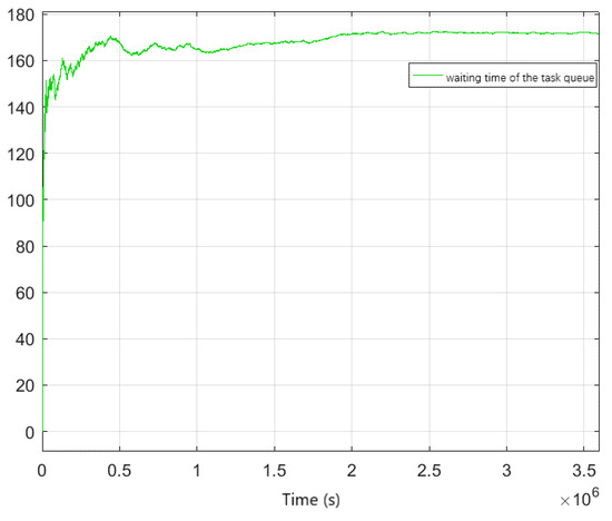
Figure 6.
The waiting time curve of the task queue.
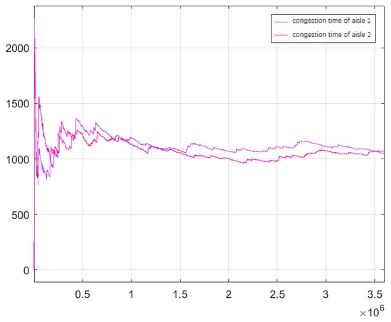
Figure 7.
The congestion time curves of the aisles.
The above two curves show that the operation mechanism of the simulation model is effective and reliable. The accuracy of the theoretical model is measured by the relative error ,
where represents the result of the theoretical model and represents the result of the simulation model. Table 3 and Table 4 record the mean value and change range of .
Table 3.
Comparison between simulation and theoretical model.
Table 4.
Comparison between simulation and theoretical model.
According to the above two tables, the average absolute error was obtained. The error of task waiting queue length was . The error of AGV utilization was . The error of the order throughput time was . The error of congestion time was . The results show that the theoretical model can effectively evaluate the performance of the AGV system considering congestion factors. The original data can also be obtained from the following link: https://icloud.qd.sdu.edu.cn:7777/link/40484921320252C06D9ADAF0BC61DCFD (accessed on 6 November 2021).
4.2. Result Analysis
4.2.1. The Optimal Number of AGVs Configuration
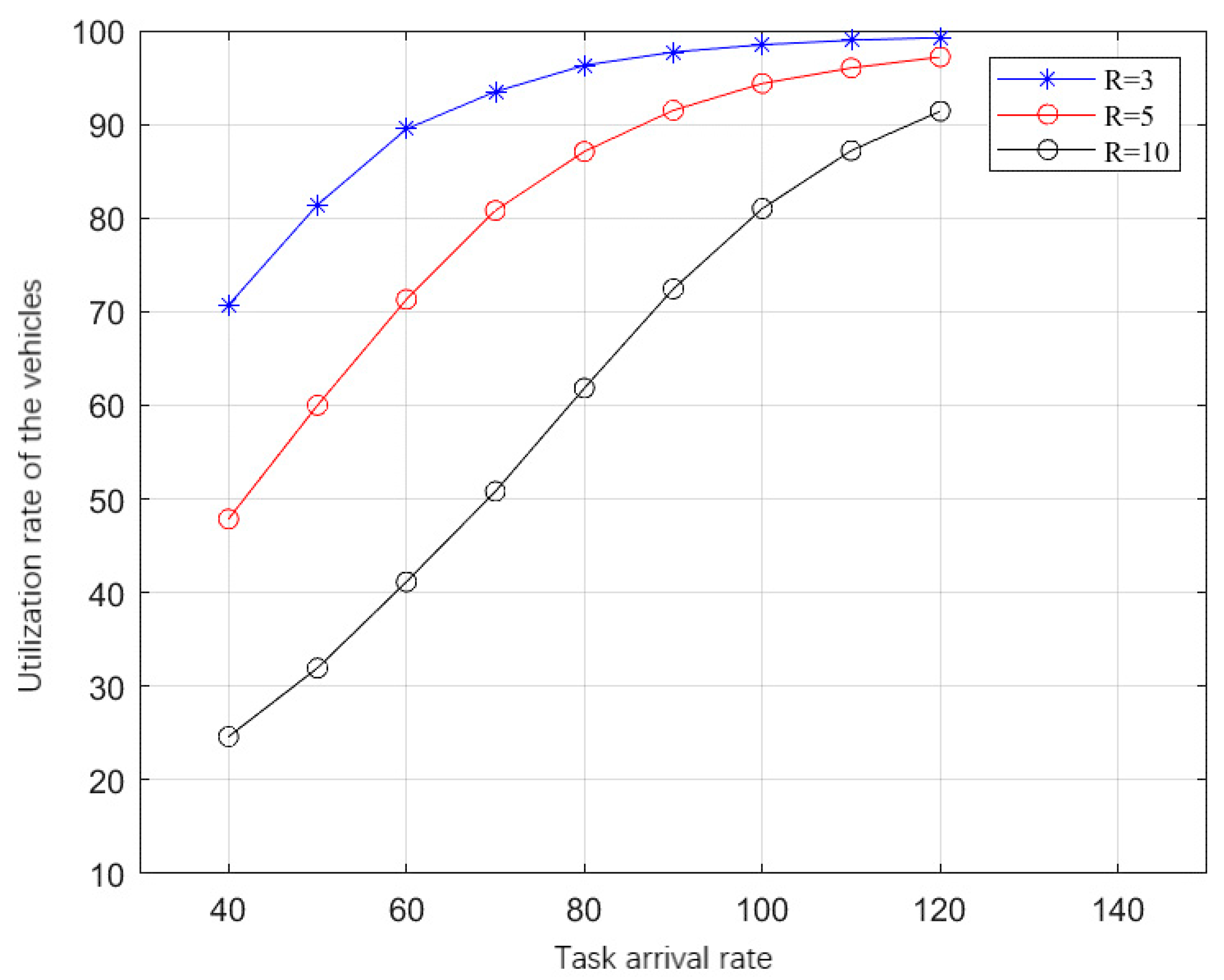
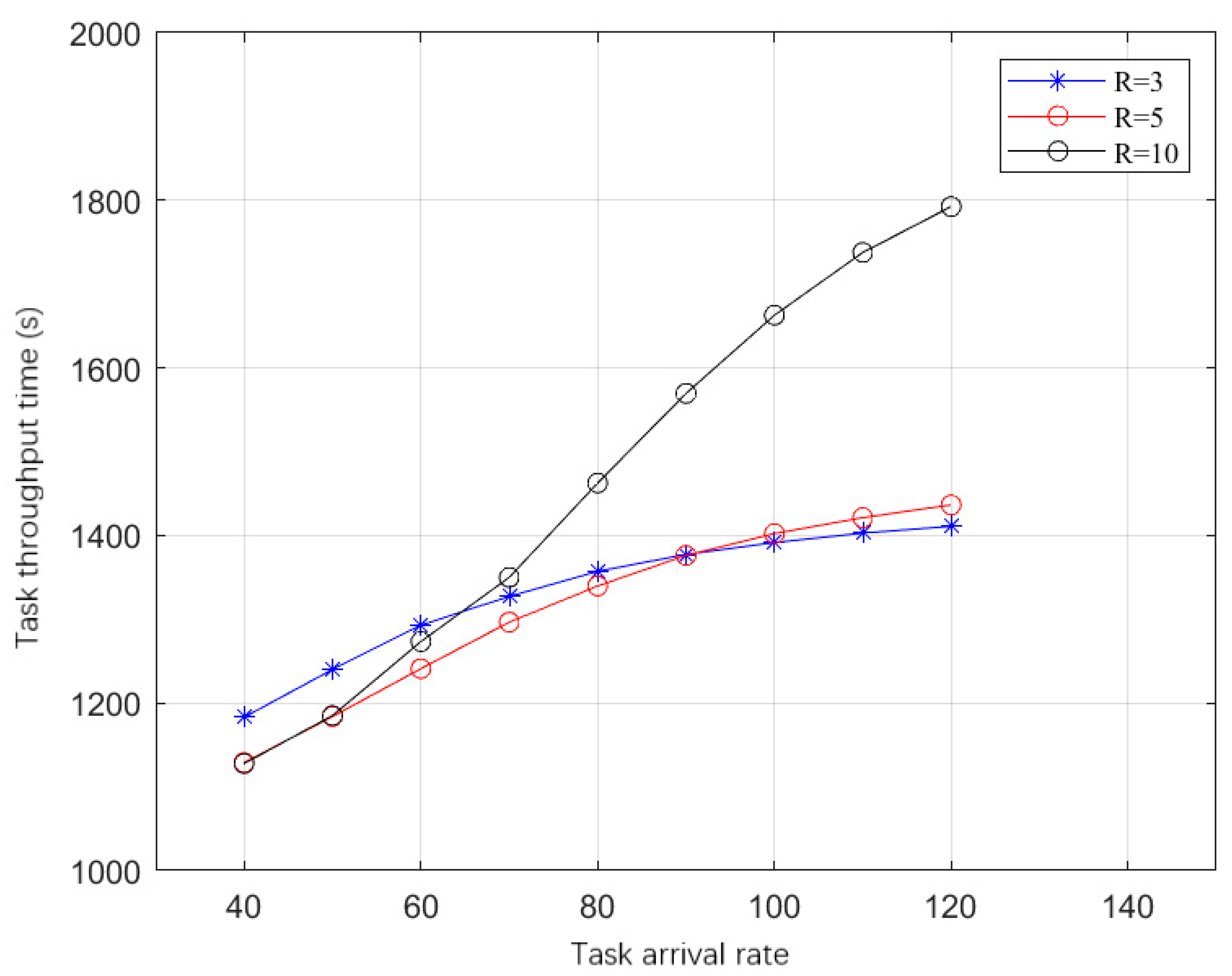
The number of AGVs configuration needs to consider two aspects, one is the engineering requirements, the other is the task arrival rate. The utilization rate of AGVs is generally required to be kept within a certain range, most of which are 60~90%. When the number of vehicles is low, the vehicle utilization will become too high and the waiting time will be longer. When the number of vehicles is high, the idle rate of vehicles will increase, resulting in a waste of resources. In order to optimize the number of AGVs, we set the length–width ratio of the warehouse as 0.5, the number of storage spaces as 2690, and the number of vehicles as 3, 5, and 10, respectively. When the task arrival rate is 40~120, the throughput time of the task and the utilization rate of the vehicles are obtained through the experiment, and the result charts are as shown below.
From Figure 8, it can be seen that the utilization rate of the vehicles increases significantly with the increase of the task arrival rate, and the fewer the number of vehicles, the higher the utilization rate. As can be seen from Figure 9, although the number of AGVs is different, the task throughput time shows an upward trend with the increase of task arrival rate. This is because task waiting time and vehicle congestion will increase as the increase of task arrival rate, and then task throughput time will increase. Through the experiment, we can conclude that the analytical model can be used to plan the minimum number of vehicles to meet the task requirements under the premise of known engineering requirements and task arrival rate.
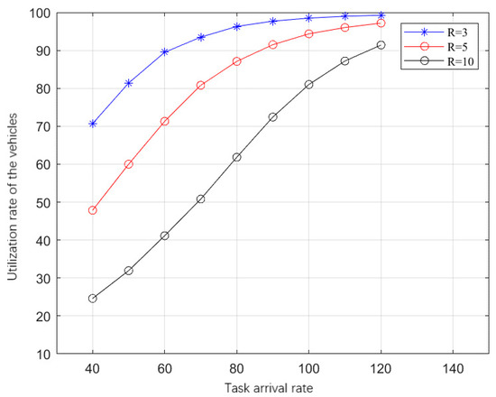
Figure 8.
The curve of the vehicle utilization rate with the task arrival rate.
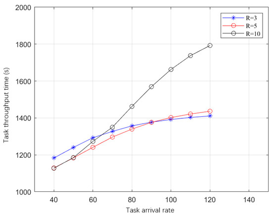
Figure 9.
The curve of the task throughput time with the task arrival rate.
4.2.2. Influence of System Structure Parameters
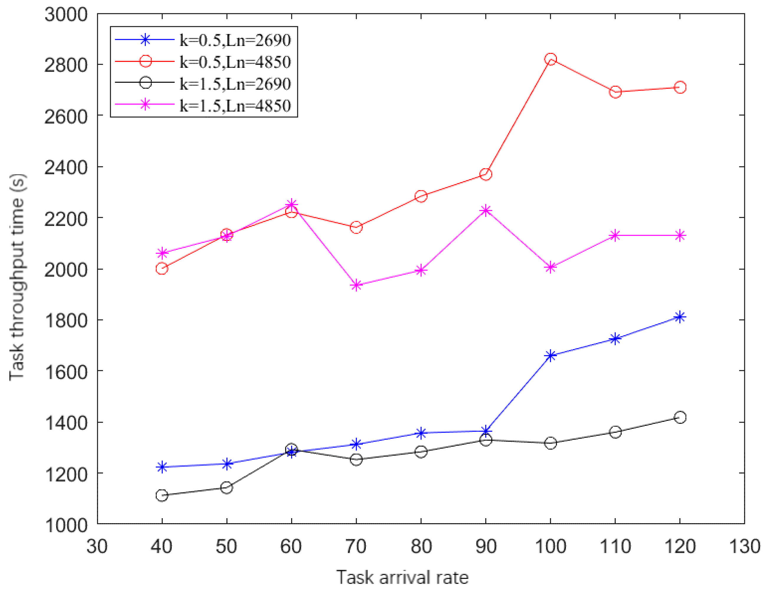
In the aspect of design, the system structure parameters will affect the performance. The specific structure parameters mainly include the length–width ratio of the warehouse and the number of storage spaces. These two parameters determine the size of the warehouse. We can analyze how these system design parameters affect the performance index through the experiments. First, the number of AGVs is set according to the conclusion of the previous part of the experiments. When the task arrival rate is 40~60, 70~90, 100~120, the number of AGVs is 3, 5, and 10 respectively. The change curve of task throughput time with task arrival rate under different size parameters of the warehouse is calculated through the analytical model, and the following result figure is obtained as follows.
It can be seen from Figure 10 that when the length–width ratio of the warehouse is fixed, the throughput time of the task increases significantly with the increase of the number of storage spaces. This is because when the number of storage spaces increases, the aisle length and cross-aisle length of the whole system increase, and the service time of AGV increases, so the throughput time will increase accordingly. The throughput time of tasks also changes significantly when the number of storage spaces is fixed, but the length–width ratio of the warehouse is changed. As shown in Figure 10, when the number of storage spaces is set as 2690, the blue curve represents the change of throughput time when the length–width ratio is 0.5 and the black curve represents the change of throughput time when the length–width ratio is 1.5. The blue curve is always above the black curve in this figure, which shows that the task throughput time is on a downward trend, that is, the performance of the system is increasing with the increase of the length–width ratio of the warehouse. Therefore, the experiment shows that the performance of the system is sensitive to the structural parameters of the system.
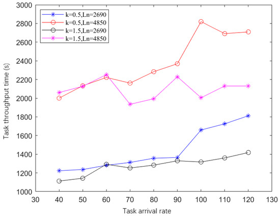
Figure 10.
The Influence of the length–width ratio and the storage spaces on system performance.
4.2.3. Influence of Congestion
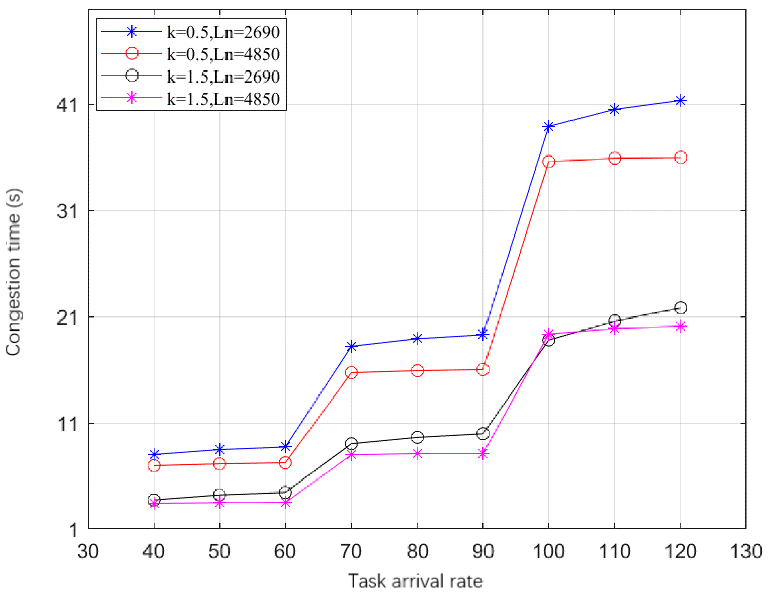
During the operation of the system, the service intensity of the system increases with the increase of the number of AGV, and the waiting time of AGV increases due to congestion. The influence of this factor on performance can be quantified by experiments. By changing the number of vehicles, the change curve of the proportion of congestion time in throughput time under the different configuration of system structure parameters is obtained. The results are shown in the figure below.
The AGV congestion is that multiple AGVs occupy the same space resource at the same time, which leads to the problem of vehicle delay. It can be seen from Figure 11 that the proportion of congestion time varies with the size of the warehouse and the number of vehicles. From the above figure, the congestion time is rising in a ladder shape with the increase of the number of vehicles. In system design, different color curves represent different design combination parameters. Among them, the magenta curve is at the bottom of all curves, which means that the length–width ratio of the warehouse is the largest, the number of storage spaces is the largest, and the congestion time is the least. The blue curve is at the top of all curves, which means that the length–width ratio of the warehouse is the smallest, the number of storage spaces is the least, and the congestion time is the most. This conclusion shows that congestion increases with the increase of warehouse size, which is also consistent with the actual vehicle operation scenario, and verifies the validity of the model to the actual system description.
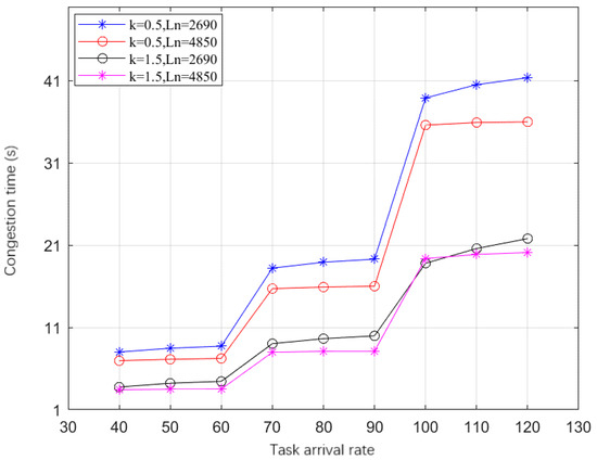
Figure 11.
The variation of the congestion time with the task arrival rate.
5. Conclusions
The demand for the transformation of fixed shelves system into AGV automatic handling system is becoming higher and higher. This paper provides a theoretical model to evaluate how to configure the number of AGVs in the shelves system with original manually driven forklifts. The theoretical model is based on a semi open-loop queuing network, which considers the arrival, queuing, served, and leaving of orders in the system and considers the influence of fixed resources in the system. The existing internal AGV vehicle resources and the arrival of external orders can be better used to describe the actual fixed shelves AGV picking system. In terms of scheduling rules, it is assumed that the vehicles entering the aisle obey the rule of last come first serve, so as to schedule the conflict problem.
Experimental and simulation results show that the model established in this paper provides a certain guiding significance in evaluating system performance and AGV vehicle quantity configuration in the fixed shelves AGV picking system. Because the introduction cost of AGV vehicles is high, it has important practical significance for solving performance evaluation and vehicle configuration in the planning and design stage.
In addition to the congestion problem caused by the normal driving of multiple AGVs in the system, some AGV faults will also cause local congestion, including communication delay, sensor interference, hardware fault, low power, etc. The faults that can be eliminated in a short time, such as communication delay, sensor interference, and low power, can be solved by improving the priority of error reporting equipment. For the model in this paper, we can evaluate the other parameters of the system by further studying the impact of faults on the service time.
Author Contributions
The author’s contributions are as follows: conceptualization, C.C.; data curation, S.W.; methodology, Y.W.; supervision, J.Z.; writing—original draft, C.C. All authors have read and agreed to the published version of the manuscript.
Funding
This research was funded by the Shandong Provincial Natural Science Foundation grant number ZR2020MF085.
Conflicts of Interest
The authors declare no conflict of interest.
References
- Bartholdi, J.J., III; Hackman, S.T. Warehouse and Distribution Science; Georgia Institute of Technology: Atlanta, GA, USA, 2008. [Google Scholar]
- Wurman, P.R. Coordinating Hundreds of Cooperative, Autonomous Vehicles in Warehouses. Ai Mag. 2008, 29, 9. [Google Scholar]
- Mountz, M.C.; D’Andrea, R.; Laplante, J.A. Inventory System with Mobile Drive Unit and Inventory Holder. U.S. Patent 7402018 B2, 22 July 2008. [Google Scholar]
- Zou, B. Study on Operational Policies Optimization in Vehicle-Based Storage and Retrieval Systems; Huazhong University of Science and Technology: Wuhan, China, 2017. [Google Scholar]
- Zou, B.; Gong, Y.; Xu, X. Assignment rules in robotic mobile fulfilment systems for online retailers. Int. J. Prod. Res. 2017, 55, 6175–6192. [Google Scholar] [CrossRef]
- Xie, L.; Thieme, N.; Krenzler, R. Efficient order picking methods in robotic mobile fulfillment systems. arXiv Prepr. 2019, arXiv:1902.03092. [Google Scholar]
- Dou, J.; Chen, C.; Pei, Y. Genetic Scheduling and Reinforcement Learning in Multirobot Systems for Intelligent Warehouses. Math. Probl. Eng. Theory Methods Appl. 2015, 2015 Pt 25, 597956. [Google Scholar] [CrossRef] [Green Version]
- Zhang, J.; Yang, F.; Weng, X. A Building-Block-Based Genetic Algorithm for Solving the Robots Allocation Problem in a Robotic Mobile Fulfilment System. Math. Probl. Eng. 2019, 2019, 6153848. [Google Scholar] [CrossRef] [Green Version]
- Merschformann, M.; Lamballais, T.; Koster, M.D. Decision rules for robotic mobile fulfillment systems. Oper. Res. Perspect. 2019, 6, 100–128. [Google Scholar] [CrossRef]
- Roy, D.; Nigam, S.; Koster, R.D. Robot-storage zone assignment strategies in mobile fulfillment systems. Transp. Res. Part E Logist. Transp. Rev. 2019, 122, 119–142. [Google Scholar] [CrossRef]
- Zhe, Y.; Gong, Y.Y. Bot-In-Time Delivery for Robotic Mobile Fulfillment Systems. IEEE Trans. Eng. Manag. 2017, 64, 83–93. [Google Scholar]
- Lienert, T.; Staab, T.; Ludwig, C. Simulation-based Performance Analysis in Robotic Mobile Fulfilment Systems—Analyzing the Throughput of Different Layout Configurations. In Proceedings of the 8th International Conference on Simulation and Modeling Methodologies, Technologies and Applications—SIMULTECH, Porto, Portugal, 29–31 July 2018. [Google Scholar]
- Zi, L.; Gao, B. Performance Estimating in an Innovative AGVs-based Parcel Sorting System Considering the Distribution of Destinations. In Proceedings of the 2020 IEEE 16th International Conference on Automation Science and Engineering (CASE), Hong Kong, China, 20–21 August 2020. [Google Scholar]
- Koo, P.H.; Jang, J.; Suh, J. Estimation of part waiting time and fleet sizing in AGV systems. Int. J. Flex. Manuf. Syst. 2004, 16, 211–228. [Google Scholar] [CrossRef]
- Cui, W.; Wang, H.; Jan, B. Simulation Design of AGVS Operating Process in Manufacturing Workshop. In Proceedings of the 2019 34rd Youth Academic Annual Conference of Chinese Association of Automation (YAC), Jinzhou, China, 6–8 June 2019. [Google Scholar]
- Chen, C.; Lee, K.T. Using queuing theory and simulated annealing to design the facility layout in an AGV-based modular manufacturing system. Int. J. Prod. Res. 2019, 57, 5538–5555. [Google Scholar] [CrossRef]
- Azenha, A.; Carvalho, A. A neural network approach for AGV localization using trilateration. In Proceedings of the 35th Annual Conference of IEEE Industrial Electronics, Porto, Portugal, 3–5 November 2009. [Google Scholar]
- Kemény, Z. Human–robot collaboration in manufacturing: A multi-agent view. In Advanced Human-Robot. Collaboration in Manufacturing; Springer: Cham, Switzerland, 2021; pp. 3–41. [Google Scholar]
- Zacharaki, A.; Kostavelis, I.; Gasteratos, A.; Dokas, I. Safety bounds in human robot interaction: A survey. Saf. Sci. 2020, 127, 104667. [Google Scholar] [CrossRef]
- Pratama, P.S.; Setiawan, Y.D.; Kim, D.H. Fault detection algorithm for automatic guided vehicle based on multiple positioning modules. In Proceedings of the 2014 International Conference on Advances in Computing, Communications and Informatics (ICACCI), Delhi, India, 24–27 September 2014. [Google Scholar]
- Witczak, M.; Majdzik, P.; Stetter, R. Multiple AGV fault-tolerant within an agile manufacturing warehouse. IFAC-Pap. 2019, 52, 1914–1919. [Google Scholar] [CrossRef]
- Liu, Z.; Wang, Y.; Jin, M. Energy consumption model for shuttle-based Storage and Retrieval Systems. J. Clean. Prod. 2021, 282, 124480. [Google Scholar] [CrossRef]
- Wang, Y.; Liu, Z.; Huang, K. Model and solution approaches for retrieval operations in a multi-tier shuttle. Comput. Ind. Eng. 2020, 141, 106283. [Google Scholar] [CrossRef]
- Zou, B.; Xu, X.; Gong, Y.Y. Evaluating battery charging and swapping strategies in a robotic mobile fulfillment system. Eur. J. Oper. Res. 2018, 267, 733–753. [Google Scholar] [CrossRef]
Publisher’s Note: MDPI stays neutral with regard to jurisdictional claims in published maps and institutional affiliations. |
© 2021 by the authors. Licensee MDPI, Basel, Switzerland. This article is an open access article distributed under the terms and conditions of the Creative Commons Attribution (CC BY) license (https://creativecommons.org/licenses/by/4.0/).