Article

Global Dynamics of a Stochastic Viral Infection Model with Latently Infected Cells

by
Chinnathambi Rajivganthi
1 and
Fathalla A. Rihan
2,*
1
School of Applied Mathematics, Getulio Vargas Foundation, Rio de Janeiro 22250-900, RJ, Brazil
2
Department of Mathematical Sciences, College of Science, United Arab Emirates University, Al-Ain 15551, United Arab Emirates
*
Author to whom correspondence should be addressed.
Appl. Sci. 2021, 11(21), 10484; https://doi.org/10.3390/app112110484
Submission received: 17 September 2021 / Revised: 2 November 2021 / Accepted: 5 November 2021 / Published: 8 November 2021
(This article belongs to the Special Issue Dynamic Models of Biology and Medicine, Volume III)

Abstract

:
In this paper, we study the global dynamics of a stochastic viral infection model with humoral immunity and Holling type II response functions. The existence and uniqueness of non-negative global solutions are derived. Stationary ergodic distribution of positive solutions is investigated. The solution fluctuates around the equilibrium of the deterministic case, resulting in the disease persisting stochastically. The extinction conditions are also determined. To verify the accuracy of the results, numerical simulations were carried out using the Euler–Maruyama scheme. White noise’s intensity plays a key role in treating viral infectious diseases. The small intensity of white noises can maintain the existence of a stationary distribution, while the large intensity of white noises is beneficial to the extinction of the virus.

1. Introduction

Mathematical models have been introduced to define the within-host dynamical behaviors of various viral infections, mainly focusing on virus-to-cell spread in the bloodstream, such as human immunodeficiency virus (HIV) [1], COVID-19 [2,3], hepatitis C virus (HCV) [4,5], hepatitis B virus (HBV) [6], human T cell lymphotropic virus I (HTLV-1) [7], etc. Those classical viral infection models are composed of interactions among susceptible cells, infected target cells, and free viruses. Further, some authors include latent infection to describe the mechanism of latency. Wang et al. [8] investigated the HIV model with latent infection incorporating both modes of time delays, transmissions between viral entry and viral production or integration and also discussed the basic reproductive number and existence results of asymptotic stability of the endemic equilibrium points. Wen et al. [9] studied the virus-to-cell and cell-to-cell HIV virus transmission dynamics with latently infected cells. Pan et al. [10] discussed the HCV infection model, which includes the routes of infection and spread, like, virus-to-cell and cell-to-cell transmission dynamics, and explained numerically the four different HCV models.
The virus can weaken and suppress the immune response, which leads to persistent infections. Immune system response refers to the process that when the virus entry to the human body, the immune system receives the signal of virus attack and spreads it to the immune organs, which secrete lymphocytes to purge the virus. Moreover, the adaptive immune response plays a crucial role in the control of the infection process. When a virus spreads to the human body, the human body produces double modes of immune responses: one is the B-cell, which causes a humoral immune response and the second is the Cytotoxic T Lymphocyte (CTL), which causes a cellular immune response. Previous studies have showed that the humoral immune response is more active than the cellular immune responses. Elaiw et al. [11] discussed the dynamical behaviors of viral infection models with latently infected cells, humoral immune response, and general nonlinear incidence rate function. The authors in [12] investigated the global asymptotic stability of a reaction–diffusion virus infection model with homogeneous environments, nonlinear incidence in heterogeneous, and humoral immunity. Wang et al. [13] discussed the global stability results of HIV viral infection model with latently infected cells, B-cell immune response, Beddington–DeAngelis functional response, and various time delays. The authors in [14] reported the stability and bifurcation results of generalized viral infection system with humoral immunity and distributed delays in virus production and cell infection, and used time lags to describe the time needed to activate the immune response.
Stochastic modeling of viral infectious disease plays an important role and gives an extra degree of realism when compared to their corresponding deterministic models [15]. Generally, viral infection models, infective virus particles, and different cells reacting in the same environment can often provide different results. In reality, due to continuous fluctuations in the environment, the parameters involved in the system always fluctuate around some average values ([16,17,18]). Wang et al. [19] formulated the HIV viral infection model with latently infectious and random noise and also studied the existing results of stationary distribution/stochastic persistence. The authors in [20] discussed the stationary distribution and extinction results of stochastic HBV viral infection model with a time lag in the transmission coefficient make the periodic outbreaks. Sun et al. [21] investigated the existence of solution for the stochastic viral infectious system with CTL responses and distributed delay, moreover, the diseases will be eradicated while the stochastic reproductive number is less than one and if the stochastic reproductive ratio is greater than one, the viral infection will be stochastic persistence/ergodic stationary distribution. Rihan et al. [22] derived the existence of solution and stationary distribution of stochastic HBV model with intracellular delay, moreover, the solution fluctuates around endemic equilibrium of the corresponding deterministic model and leads to the stochastic persistence of the disease.
Motivated by the above-mentioned studies, in this paper, we formulate and analyze the dynamical behaviors of a virus–immune system with white noise. The presence and uniqueness of the global non-negative solution of the stochastic viral infection model with a Holling type II functional response is investigated. Using a stochastic Lyapunov function combined with Ito’s formula, we provide a sufficient condition for determining the existing results of stationary distribution and extinction of such considered model. The rest of this paper is organized as follows: In Section 2, we formulate the viral infection model and study the existence of global positive solution. Stationary distribution and extinction results of such a model are derived in Section 3 and Section 4. Some numerical simulations are given in Section 5 to verify the obtained theoretical results. Section 6 contains the conclusion.

2. Model Formulation

In the process of viral infection, the immune system plays a critical role. Viral dynamics can be modeled properly to provide insights into understanding the disease and the clinical treatments used to treat it. In adaptive immune responses, lymphocytes are responsible for specificity and memory. The two main types of lymphocytes are B cells and T cells. The function of T cells is to recognize and kill infected cells, while the function of B cells is to produce antibodies to neutralize the viruses. Researchers have studied the effects of immune responses such as CTL responses and antibody responses [23,24,25,26,27]. Some other researchers have also taken into account the effect of CTL responses and intracellular delays [5,28,29]. The mathematical model that describes the effect of humoral immune response on virus dynamics is presented in [27]
x ˙ ( t ) = λ d 1 x ( t ) β 11 x ( t ) v ( t ) β 22 x ( t ) y ( t ) , y ˙ ( t ) = β 1 x ( t ) v ( t ) + β 2 x ( t ) y ( t ) a y ( t ) , v ˙ ( t ) = k y ( t ) μ v ( t ) ξ v ( t ) w ( t ) , w ˙ ( t ) = g v ( t ) w ( t ) h w ( t ) .
This model consists of uninfected target cells x ( t ) , actively infected cells y ( t ) , free viruses v ( t ) , and antibodies/B cells w ( t ) . The uninfected cells x ( t ) are produced at a rate constant λ and death rate d 1 . β 11 is the infection rate by free virus and uninfected cells being converted to productively infected ones at a rate β 22 per both cells. a , μ , h are the death rate of infected cells, free virus particles, and antibodies/B cells, respectively. Free virus particle are produced from productively infected cells at the rate k and ξ is the rate of neutralization by antibodies. g is the rate of antibodies activated against the virus.
Herein, we upgrade model (1) to include the latent infection component. We assume that the uninfected cell x ( t ) gets infected by a free virus v ( t ) or by direct contact with an infected cell y ( t ) at the rate β 1 x ( t ) v ( t ) 1 + v ( t ) + β 2 x ( t ) y ( t ) 1 + y ( t ) with a Holling type II functional response. β 1 > 0 and β 2 > 0 represent the virus to cell infection rate and cell to cell transmission rate, respectively [30]. We also assume that ( 1 φ ) and φ ( 0 , 1 ) are the proportions of infection that lead to latency and productivity, respectively. Additionally, in order to reflect a more realistic situation of disease development, we incorporated the effect of randomization within the host by introducing nonlinear perturbations on the natural death rate with white noise into each equation. Therefore, the extended model takes the following form:
d x ( t ) = ( λ d 1 x ( t ) β 1 x ( t ) v ( t ) 1 + v ( t ) β 2 x ( t ) y ( t ) 1 + y ( t ) ) d t + σ 1 x ( t ) d W 1 ( t ) , d l ( t ) = ( ( 1 φ ) β 1 x ( t ) v ( t ) 1 + v ( t ) + β 2 x ( t ) y ( t ) 1 + y ( t ) ( m + γ ) l ( t ) ) d t + σ 2 l ( t ) d W 2 ( t ) , d y ( t ) = ( φ β 1 x ( t ) v ( t ) 1 + v ( t ) + β 2 x ( t ) y ( t ) 1 + y ( t ) + γ l ( t ) a y ( t ) ) d t + σ 3 y ( t ) d W 3 ( t ) , d v ( t ) = ( k y ( t ) μ v ( t ) ξ v ( t ) w ( t ) ) d t + σ 4 v ( t ) d W 4 ( t ) , d w ( t ) = ( g v ( t ) w ( t ) h w ( t ) ) d t + σ 5 w ( t ) d W 5 ( t ) ,
with initial values x ( 0 ) > 0 , l ( 0 ) > 0 , y ( 0 ) > 0 , v ( 0 ) > 0 , w ( 0 ) > 0 . l ( t ) denotes the concentrations of infected cells in latent stage at t. m be the death rate of l ( t ) and latent infection become productively infected cells at the rate γ . σ 1 2 , σ 2 2 , σ 3 2 , σ 4 2 , σ 5 2 are intensities of the environmental white noises. W 1 ( t ) , W 2 ( t ) , W 3 ( t ) , W 4 ( t ) , W 5 ( t ) are mutually independent standard Brownian motions with W i ( 0 ) = 0 ( i = 1 , 2 , 3 , 4 , 5 ). We define the basic concepts of probability theory and SDEs. Let ( Ω , F , { F t } t 0 , P ) be complete probability space with filtration { F t } t 0 satisfies the usual conditions and see more details about Ito’s formula (see [31,32,33]).
Definition 1.
Let U denote the family of all continuous non-decreasing functions u 1 : R + R + such that u 1 ( 0 ) = 0 and u 1 ( r ) > 0 if r > 0 . For h > 0 , let S h = { y 1 R n : | y 1 | < h } . A continuous function V ( y 1 , t ) defined on S h × [ t 0 , ) is said be Lyapunov function if
(i).
V ( 0 , t ) = 0 and for some u 1 U , u 1 ( | y 1 | ) V ( y 1 , t ) , for every ( y 1 , t ) S h × [ t 0 , ) .
(ii).
V ( y 1 , t ) C 2 , 1 ( S h × [ t 0 , ) , R + ) such that L V ( y 1 , t ) 0 .
Let y 1 ( t ) be a regular time-homogeneous Markov process in R n defined by SDE
d y 1 ( t ) = f ( y 1 ( t ) ) d t + g ( y 1 ( t ) ) d W ( t ) .
The diffusion matrix of the process y 1 ( t ) is described as A ( y 1 ) = ( b i j ( y 1 ) ) , b i j ( y 1 ) = g i ( y 1 ) g j ( y 1 ) .
Lemma 1.
([34]) The Markov process y 1 ( t ) has a unique ergodic stationary distribution π ( · ) if there exists a bounded open domain D R n with regular boundary Γ , having the following properties:
  • the diffusion matrix A ( y 1 ) is strictly positive definite for all y 1 D .
  • there exists a non-negative C 2 function V such that L V is negative for any R n \ D .
Theorem 1.
Assume that g < ξ < h , β 1 k < μ + g , ( β 2 + 1 ) < a k , the model (2) has a unique positive solution ( x ( t ) , l ( t ) , y ( t ) , v ( t ) , w ( t ) ) on t 0 with ( x ( 0 ) , l ( 0 ) , y ( 0 ) , v ( 0 ) , w ( 0 ) ) R + 5 , and the solution will remain in R + 5 with probability 1.
Proof. 
Basically, the coefficients of the system (2) satisfy the local Lipschitz condition, then (2) has a unique local solution ( x ( t ) , l ( t ) , y ( t ) , v ( t ) , w ( t ) ) on [ 0 , τ e ] , where τ e is an exposure time. Then, we prove that τ e = + . Let us follow the similar proof of Theorem 3.1 in [32]. The major step is to describe a non-negative C 2 function V : R + 5 R + such that lim h 1 , ( x , l , y , v , w ) R + 5 \ D h 1 inf V ( x , l , y , v , w ) = + , a n d L V ( x , l , y , v , w ) K , where D h 1 = ( 1 h 1 , h 1 ) × ( 1 h 1 , h 1 ) × ( 1 h 1 , h 1 ) × ( 1 h 1 , h 1 ) × ( 1 h 1 , h 1 ) , and K is non-negative constant. Define a function V : R + 5 R + as follows
V ( x , l , y , v , w ) = ( x 1 l n x ) + ( l 1 l n l ) + ( y 1 l n y ) + ( v 1 l n v ) + ( w 1 l n w ) .
The non-negativity of this function can be seen from ϑ 1 l n ϑ 0 , ϑ > 0 . By applying the Ito’s formula, we can obtain
d V ( x , l , y , v , w ) = L V ( x , l , y , v , w ) d t + σ 1 ( x 1 ) d W 1 ( t ) + σ 2 ( l 1 ) d W 2 ( t ) + σ 3 ( y 1 ) d W 3 ( t ) + σ 4 ( v 1 ) d W 4 ( t ) + σ 5 ( w 1 ) d W 5 ( t ) , L V ( x , l , y , v , w ) = ( 1 1 x ) ( λ d 1 x ( t ) β 1 x ( t ) v ( t ) 1 + v ( t ) β 2 x ( t ) y ( t ) 1 + y ( t ) ) + ( 1 1 l ) ( ( 1 φ ) β 1 x ( t ) v ( t ) 1 + v ( t ) + β 2 x ( t ) y ( t ) 1 + y ( t ) ( m + γ ) l ( t ) ) + ( 1 1 y ) ( φ β 1 x ( t ) v ( t ) 1 + v ( t ) + β 2 x ( t ) y ( t ) 1 + y ( t ) + γ l ( t ) a y ( t ) ) + ( 1 1 v ) ( k y ( t ) μ v ( t ) ξ v ( t ) w ( t ) ) + ( 1 1 w ) ( g v ( t ) w ( t ) h w ( t ) ) + σ 1 2 + σ 2 2 + σ 3 2 + σ 4 2 + σ 5 2 2 , λ + d 1 + m + γ + a + μ + h + ( ξ h ) w + ( g ξ ) v w + ( β 1 k ( μ + g ) ) v + ( ( β 2 + 1 ) k a ) y + σ 1 2 + σ 2 2 + σ 3 2 + σ 4 2 + σ 5 2 2 .
Using the assumptions g < ξ < h , β 1 k < μ + g , ( β 2 + 1 ) < a k , there exists a positive constant K such that L V K . The rest of proof follows that of [31,32] and hence, is omitted.  □

3. Existence of Ergodic Stationary Distribution

Here, we discuss the stationary distribution results for the model (2), which helps to identify whether the diseases are persistent or can be eradicated.
Theorem 2.
Assume that R 0 s : = λ γ k β 1 ( 1 φ ) d 1 a ^ γ ^ μ ^ > 1 , then for any ( ( x ( 0 ) , l ( 0 ) , y ( 0 ) , v ( 0 ) , w ( 0 ) ) R + 5 , the model ( 2 ) has a unique ergodic stationary distribution π ( · ) , where γ ^ = m + γ + σ 2 2 2 , a ^ = a + σ 3 2 2 , μ ^ = μ + σ 4 2 2 .
Proof. 
The diffusion matrix of (2) is calculated as below
A = σ 1 2 x 2 0 0 0 0 0 σ 2 2 l 2 0 0 0 0 0 σ 3 2 y 2 0 0 0 0 0 σ 4 2 v 2 0 0 0 0 0 σ 5 2 w 2 ,
which is positive definite for any compact subset of R + 5 , the condition (i) in Lemma 1 is verified.
Define the C 2 function V : R + 5 R as
V ( x , l , y , v , w ) = M l n x c 1 l n l c 2 l n y c 3 l n v l n w l n x l n l l n y l n v + 1 ρ + 1 ( x + l + y + v + w ) ρ + 1 , = M V 1 + V 2 + V 3 + V 4 + V 5 + V 6 ,
where c 1 = λ β 1 γ k ( 1 φ ) γ ^ 2 a ^ μ ^ , c 2 = λ β 1 γ k ( 1 φ ) γ ^ a ^ 2 μ ^ , c 3 = λ β 1 γ k ( 1 φ ) γ ^ a ^ μ ^ 2 , 0 < ρ < 1 satisfying η ρ 2 ( σ 1 2 σ 2 2 σ 3 2 σ 4 2 σ 5 2 ) > 0 and M > 0 is constant, satisfying the condition M ν + N 1 2 , N 1 = d 1 + ( M + 1 ) σ 1 2 2 + M h + M σ 5 2 2 + ( M + 1 ) β 2 y + β 1 v + N 2 + m + γ + σ 2 2 2 + a + σ 3 2 2 + μ + σ 4 2 2 and ν = d 1 R 0 s 1 > 0 . Further, V ( x , l , y , v , w ) is not only continuous, but also goes to + as ( x , l , y , v , w ) tends to the boundary of R + 5 and ( x , l , y , v , w ) . V must have a minimum point ( x ( 0 ) , l ( 0 ) , y ( 0 ) , v ( 0 ) , w ( 0 ) ) in the interior of R + 5 . Define a C 2 function V ˜ : R + 5 R + as
V ˜ ( x , l , y , v , w ) = V ( x , l , y , v , w ) V ( x ( 0 ) , l ( 0 ) , y ( 0 ) , v ( 0 ) , w ( 0 ) ) .
Applying Ito’s formula L on the functions V 1 , , V 6 and assume β 1 < g < ξ , k < a and η = max { d 1 , m , a , μ , h }
L V 1 λ x c 1 l ( 1 φ ) β 1 x v γ l c 2 y k y c 3 v + d 1 + β 2 y + c 1 ( m + γ ) + a c 2 + μ c 3 + ξ w c 3 ( g β 1 ) v + h + σ 1 2 + c 1 σ 2 2 + c 2 σ 3 2 + c 3 σ 4 2 + σ 5 2 2 , 4 c 1 c 2 c 3 λ ( 1 φ ) β 1 γ k 4 + d 1 + σ 1 2 2 + c 1 ( m + γ + σ 2 2 2 ) + c 2 ( a + σ 3 2 2 ) + c 3 ( μ + σ 4 2 2 ) + h + σ 5 2 2 + β 2 y + ξ w c 3 , λ ( 1 φ ) β 1 γ k γ ^ a ^ μ ^ + d 1 + σ 1 2 2 + h + σ 5 2 2 + β 2 y + ξ w c 3 , ν + σ 1 2 2 + h + σ 5 2 2 + β 2 y + ξ w c 3 ,
L V 2 λ x + d 1 + β 1 v + β 2 y + σ 1 2 2 ,
L V 3 = 1 l ( 1 φ ) β 1 x v 1 + v + β 2 x y 1 + y + m + γ + σ 2 2 2 ,
L V 4 = φ β 1 x v y ( 1 + v ) φ β 2 x 1 + y γ l y + a + σ 3 2 2 ,
L V 5 = k y v + μ + ξ w + σ 4 2 2 ,
L V 6 ( x + l + y + v + w ) ρ [ λ η ( x + l + y + v + w ) ] + ρ 2 ( x + l + y + v + w ) ρ 1 × [ σ 1 2 x 2 + σ 2 2 l 2 + σ 3 2 y 2 + σ 4 2 v 2 + σ 5 2 w 2 ] , ( x + l + y + v + w ) ρ [ λ η ( x + l + y + v + w ) ] + ρ 2 ( x + l + y + v + w ) ρ + 1 × ( σ 1 2 σ 2 2 σ 3 2 σ 4 2 σ 5 2 ) , λ ( x + l + y + v + w ) ρ ( x + l + y + v + w ) ρ + 1 [ η ρ 2 ( σ 1 2 σ 2 2 σ 3 2 σ 4 2 σ 5 2 ) ] , N 2 1 2 [ η ρ 2 ( σ 1 2 σ 2 2 σ 3 2 σ 4 2 σ 5 2 ) ] ( x ρ + 1 + l ρ + 1 + y ρ + 1 + v ρ + 1 + w ρ + 1 ) ,
where
N 2 = sup ( x , l , y , v , w ) R + 5 { λ ( x + l + y + v + w ) ρ 1 2 [ η ρ 2 ( σ 1 2 σ 2 2 σ 3 2 σ 4 2 σ 5 2 ) ] ( x + l + y + v + w ) ρ + 1 } < .
From Equations (4)–(9), we have
L V ˜ λ x M ν + ( M c 3 + 1 ) ξ w 1 l ( 1 φ ) β 1 x v φ β 2 x 1 + y k y v 1 4 [ η ρ 2 ( σ 1 2 σ 2 2 σ 3 2 σ 4 2 σ 5 2 ) ] ( x ρ + 1 + l ρ + 1 + y ρ + 1 + v ρ + 1 + w ρ + 1 ) 1 4 [ η ρ 2 ( σ 1 2 σ 2 2 σ 3 2 σ 4 2 σ 5 2 ) ] × ( x ρ + 1 + l ρ + 1 + y ρ + 1 + v ρ + 1 + w ρ + 1 ) + d 1 + ( M + 1 ) σ 1 2 2 + M h + M σ 5 2 2 + ( M + 1 ) β 2 y + β 1 v + N 2 + m + γ + σ 2 2 2 + a + σ 3 2 2 + μ + σ 4 2 2 .
For ϵ > 0 , define a bounded closed set
D = ( x , l , y , v , w ) R + 5 : ϵ x 1 ϵ , ϵ 5 l 1 ϵ 5 , ϵ 2 y 1 ϵ 2 , ϵ 3 v 1 ϵ 3 , ϵ w 1 ϵ .
In the set R + 5 \ D , let us choose ϵ satisfies the following conditions
λ ϵ + M 1 1 ,
( 1 φ ) β 1 ϵ + M 1 1 ,
φ β 2 ϵ 1 + ϵ 2 + M 1 1 ,
k ϵ + M 1 1 ,
0 < ϵ < 1 ( M c 3 + 1 ) ξ ,
1 4 η ρ 2 ( σ 1 2 σ 2 2 σ 3 2 σ 4 2 σ 5 2 ) 1 ϵ ρ + 1 + M 1 1 ,
1 4 η ρ 2 ( σ 1 2 σ 2 2 σ 3 2 σ 4 2 σ 5 2 ) 1 ϵ 2 ( ρ + 1 ) + M 1 1 ,
1 4 η ρ 2 ( σ 1 2 σ 2 2 σ 3 2 σ 4 2 σ 5 2 ) 1 ϵ 3 ( ρ + 1 ) + M 1 1 ,
1 4 η ρ 2 ( σ 1 2 σ 2 2 σ 3 2 σ 4 2 σ 5 2 ) 1 ϵ 5 ( ρ + 1 ) + M 1 1 ,
where M 1 = sup ( x , l , y , v , w ) R + 5 ( M c 3 + 1 ) ξ w 1 4 η ρ 2 ( σ 1 2 σ 2 2 σ 3 2 σ 4 2 σ 5 2 ) ( x ρ + 1 + l ρ + 1 + y ρ + 1 + v ρ + 1 + w ρ + 1 ) + d 1 + ( M + 1 ) σ 1 2 2 + M h + M σ 5 2 2 + ( M + 1 ) β 2 y + β 1 v + N 2 + m + γ + σ 2 2 2 + a + σ 3 2 2 + μ + σ 4 2 2 . We need to verity the Lemma 1, to show that L V ˜ 1 for ( x , l , y , v , w ) R + 5 \ D and R + 5 \ D = i = 1 10 D i , where
D 1 = { ( x , l , y , v , w ) R + 5 ; 0 < x < ϵ } , D 2 = { ( x , l , y , v , w ) R + 5 ; 0 < l < ϵ 5 , x ϵ , v ϵ 3 } , D 3 = { ( x , l , y , v , w ) R + 5 ; 0 < y < ϵ 2 , x ϵ } , D 4 = { ( x , l , y , v , w ) R + 5 ; 0 < v < ϵ 3 , y ϵ 2 } , D 5 = { ( x , l , y , v , w ) R + 5 ; 0 < w < ϵ } , D 6 = { ( x , l , y , v , w ) R + 5 ; x > 1 ϵ } , D 7 = { ( x , l , y , v , w ) R + 5 ; l > 1 ϵ 5 } , D 8 = { ( x , l , y , v , w ) R + 5 ; y > 1 ϵ 2 } D 9 = { ( x , l , y , v , w ) R + 5 ; v > 1 ϵ 3 } , D 10 = { ( x , l , y , v , w ) R + 5 ; w > 1 ϵ } .
Case (i) For ( x , l , y , v , w ) D 1 , by (10) we get
L V ˜ λ x + ( M c 3 + 1 ) ξ w 1 4 η ρ 2 ( σ 1 2 σ 2 2 σ 3 2 σ 4 2 σ 5 2 ) ( x ρ + 1 + l ρ + 1 + y ρ + 1 + v ρ + 1 + w ρ + 1 ) + d 1 + ( M + 1 ) σ 1 2 2 + M h + M σ 5 2 2 + ( M + 1 ) β 2 y + β 1 v + N 2 + m + γ + σ 2 2 2 + a + σ 3 2 2 + μ + σ 4 2 2 , λ ϵ + M 1 1 ,
which obtained from (11).
Case (ii) For ( x , l , y , v , w ) D 2 , we have
L V ˜ 1 l ( 1 φ ) β 1 x v + M 1 , 1 ϵ ( 1 φ ) β 1 + M 1 1 ,
which is obtained from (12).
Case (iii) For ( x , l , y , v , w ) D 3 , we have
L V ˜ φ β 2 x 1 + y + M 1 , φ β 2 ϵ 1 + ϵ 2 + M 1 1 ,
which is obtained from (13).
Case (iv) For ( x , l , y , v , w ) D 4 , we have
L V ˜ k y v + M 1 , k ϵ + M 1 1 ,
which is obtained from (14).
Case (v) For ( x , l , y , v , w ) D 5 , we have
L V ˜ M ν + ( M c 3 + 1 ) ξ w + N 1 , M ν + ( M c 3 + 1 ) ξ ϵ + N 1 < 1 ,
which is obtained from (15) and M ν + N 1 2 .
Case (vi) For ( x , l , y , v , w ) D 6 , we get
L V ˜ 1 4 [ η ρ 2 ( σ 1 2 σ 2 2 σ 3 2 σ 4 2 σ 5 2 ) ] x ρ + 1 + M 1 , 1 4 [ η ρ 2 ( σ 1 2 σ 2 2 σ 3 2 σ 4 2 σ 5 2 ) ] 1 ϵ ρ + 1 + M 1 1 ,
which is obtained from (16).
Case (vii) For ( x , l , y , v , w ) D 7 , it yields
L V ˜ 1 4 [ η ρ 2 ( σ 1 2 σ 2 2 σ 3 2 σ 4 2 σ 5 2 ) ] l ρ + 1 + M 1 , 1 4 [ η ρ 2 ( σ 1 2 σ 2 2 σ 3 2 σ 4 2 σ 5 2 ) ] 1 ϵ 5 ( ρ + 1 ) + M 1 1 ,
which is obtained from (19).
Case (viii) For ( x , l , y , v , w ) D 8 , we get
L V ˜ 1 4 [ η ρ 2 ( σ 1 2 σ 2 2 σ 3 2 σ 4 2 σ 5 2 ) ] y ρ + 1 + M 1 , 1 4 [ η ρ 2 ( σ 1 2 σ 2 2 σ 3 2 σ 4 2 σ 5 2 ) ] 1 ϵ 2 ( ρ + 1 ) + M 1 1 ,
which is obtained from (17).
Case (ix) For ( x , l , y , v , w ) D 9 , it yields
L V ˜ 1 4 [ η ρ 2 ( σ 1 2 σ 2 2 σ 3 2 σ 4 2 σ 5 2 ) ] v ρ + 1 + M 1 , 1 4 [ η ρ 2 ( σ 1 2 σ 2 2 σ 3 2 σ 4 2 σ 5 2 ) ] 1 ϵ 3 ( ρ + 1 ) + M 1 1 ,
which is obtained from (18).
Case (x) For ( x , l , y , v , w ) D 10 , we get
L V ˜ 1 4 [ η ρ 2 ( σ 1 2 σ 2 2 σ 3 2 σ 4 2 σ 5 2 ) ] w ρ + 1 + M 1 , 1 4 [ η ρ 2 ( σ 1 2 σ 2 2 σ 3 2 σ 4 2 σ 5 2 ) ] 1 ϵ ρ + 1 + M 1 1 ,
which is obtained from (16).
Therefore, follows the above discussion, there exists a ϵ > 0 , such that L V ˜ ( x , l , y , v , w ) 1 , for all ( x , l , y , v , w ) R + 5 \ D . Based on Lemma 1, the model (2) has a unique ergodic stationary distribution.  □

4. Extinction

Now, we establish the conditions under which extinction of the disease.
Theorem 3.
Let ( x ( t ) , l ( t ) , y ( t ) , v ( t ) , w ( t ) ) be the solution of (2), ( x ( 0 ) , l ( 0 ) , y ( 0 ) , v ( 0 ) , w ( 0 ) ) R + 5 , if R ˜ 0 s : = 3 ( β 1 + β 2 ) λ d 1 ( ( m + σ 2 2 2 ) ( ( a k ) + σ 3 2 2 ) ( μ + σ 4 2 2 ) ) < 1 , which implies that
lim t 1 t 0 t x ( s ) d s λ d 1 , lim t l ( t ) = 0 , lim t y ( t ) = 0 , lim t v ( t ) = 0 . a . s .
Proof. 
By Theorem 1, the solution of (2) is positive,
d x ( t ) ( λ d 1 x ) d t + σ 1 x d W 1 ( t ) .
Consider the auxiliary stochastic equation of the above equation
d x 1 ( t ) = ( λ d 1 x 1 ) d t + σ 1 x 1 d W 1 ( t ) , x 1 ( 0 ) = x ( 0 ) > 0 ,
we get lim t 1 t 0 t x 1 ( s ) d s = λ d 1 a . s .
Using the comparison theorem of stochastic equation [32], we get x ( t ) x 1 ( t ) a . s . Then
lim t 1 t 0 t x ( s ) d s lim t 1 t 0 t x 1 ( s ) d s = λ d 1 . a . s .
Define l n ( l ( t ) + y ( t ) + v ( t ) ) and apply the Ito’s formula, assume k < a , we get
d ( l n ( l ( t ) + y ( t ) + v ( t ) ) ) = 1 l ( t ) + y ( t ) + v ( t ) β 1 x v 1 + v + β 2 x y 1 + y m l ( a k ) y μ v ξ v w d t ( σ 2 2 l 2 + σ 3 2 y 2 + σ 4 2 v 2 ) 2 ( l + y + v ) 2 d t + σ 2 l l + y + v d W 2 ( t ) + σ 3 y l + y + v d W 3 ( t ) + σ 4 v l + y + v d W 4 ( t ) , ( β 1 + β 2 ) x d t ( m + σ 2 2 2 ) l 2 + ( ( a k ) + σ 3 2 2 ) y 2 + ( μ + σ 4 2 2 ) v 2 ( l + y + v ) 2 d t + σ 2 l l + y + v d W 2 ( t ) + + σ 3 y l + y + v d W 3 ( t ) + σ 4 v l + y + v d W 4 ( t ) , ( β 1 + β 2 ) x d t 1 3 ( ( m + σ 2 2 2 ) ( ( a k ) + σ 3 2 2 ) ( μ + σ 4 2 2 ) ) d t + σ 2 l l + y + v d W 2 ( t ) + σ 3 y l + y + v d W 3 ( t ) + σ 4 v l + y + v d W 4 ( t ) .
Taking integration from 0 to t on both sides and divide by t,
l n ( l ( t ) + y ( t ) + v ( t ) ) t l n ( l ( 0 ) + y ( 0 ) + v ( 0 ) ) t β 1 + β 2 t 0 t x ( s ) d s 1 3 ( ( m + σ 2 2 2 ) ( ( a k ) + σ 3 2 2 ) ( μ + σ 4 2 2 ) ) + σ 2 t 0 t l l + y + v d W 2 ( s ) + σ 3 t × 0 t y l + y + v d W 3 ( s ) + σ 4 t 0 t v l + y + v d W 4 ( s ) , lim t sup l n ( l ( t ) + y ( t ) + v ( t ) ) t ( β 1 + β 2 ) λ d 1 1 3 ( ( m + σ 2 2 2 ) ( ( a k ) + σ 3 2 2 ) ( μ + σ 4 2 2 ) ) , 1 3 ( R ˜ 0 s 1 ) ( ( m + σ 2 2 2 ) ( ( a k ) + σ 3 2 2 ) ( μ + σ 4 2 2 ) ) < 0 a . s .
It implies that lim t l ( t ) = 0 , lim t y ( t ) = 0 , lim t v ( t ) = 0 . a . s .  □

5. Numerical Simulations

In this section, we use Euler–Maruyama method for solving SDEs, as was discussed in detail in [32,35], to have the discretization transformation of (2), as follows
x j + 1 = x j + [ λ d 1 x j β 1 x j v j 1 + v j β 2 x j y j 1 + y j ] Δ t + σ 1 x j Δ t ζ 1 , j , l j + 1 = l j + [ ( 1 φ ) β 1 x j v j 1 + v j + β 2 x j y j 1 + y j ( m + γ ) l j ] Δ t + σ 2 l j Δ t ζ 2 , j , y j + 1 = y j + [ φ β 1 x j v j 1 + v j + β 2 x j y j 1 + y j + γ l j a y j ] Δ t + σ 3 y j Δ t ζ 3 , j , v j + 1 = v j + [ k y j μ v j ξ v j w j ] Δ t + σ 4 v j Δ t ζ 4 , j , w j + 1 = w j + [ g v j w j h w j ( t ) ] Δ t + σ 5 w j Δ t ζ 5 , j ,
where Δ t > 0 is time increment, ζ i , j , ( i = 1 , 2 , 3 , 4 , 5 ) are independent Gaussian random variables which follow the distribution N ( 0 , 1 ) .
We assign the following parameter values: λ = 10 , d = 0.1 , β 1 = 2 , β 2 = 2 , φ = 0.5 , m = 0.5 , γ = 5 , a = 10 , k = 2 , μ = 10 , ξ = 3 , g = 2 , h = 4 .
We insert the different values of the white noises to discuss dynamical behaviors for the model (2). Initially, we consider the white noise values σ 1 = 0.9 , σ 2 = 0.9 , σ 3 = 0.7 , σ 4 = 0.9 , σ 5 = 0.8 , the threshold conditions of unique stationary distribution R 0 s = 1.5886 > 1 is satisfied. Figure 1 displays the time trajectories of the corresponding deterministic model of (2), which shows a stable behavior and also shows that the uninfected cells x ( t ) , latently infected cells l ( t ) , actively infected cells y ( t ) , free virus v ( t ) , and antibodies w ( t ) of (2) fluctuate randomly with respective stochastic mean respectively.
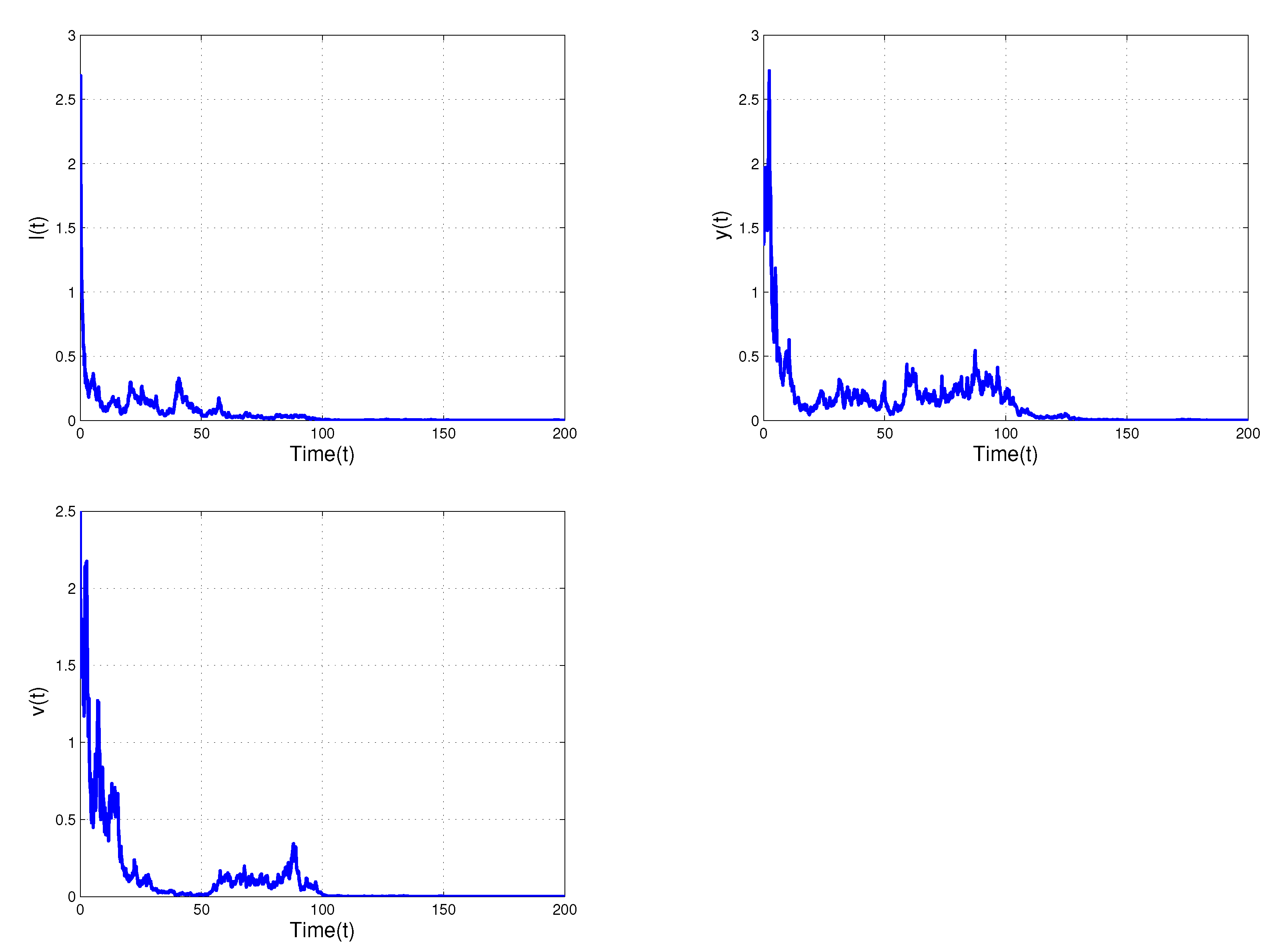
Next, we increase the white noise values σ 1 = 3.9 , σ 2 = 3.9 , σ 3 = 3.7 , σ 4 = 3.9 , σ 5 = 3.8 , we obtain the condition of extinction results in Theorem 3 such that R ˜ 0 s = 0.5665 < 1 is satisfied. Figure 2 shows that infected cells l ( t ) , actively infected cells y ( t ) , and free virus v ( t ) can all die out as the white noise value increases. As a result, this indicates that white noise intensity can significantly reduce the number of virally infected cells and inhibit the growth of infected cells, as well as eliminate all latently, actively, and free virally infected cells.
Remark 1.
Under certain conditions, the disease can be eradicated. Through numerical simulations, it has been shown that a small intensity of white noises can maintain a stationary distribution, whereas a large intensity of white noises can result in the extinction of the disease.

6. Concluding Remarks

In this work, we discussed the fluctuations in cell dynamics of a new stochastic viral infection model with latently infected cells and a Holling type II functional response. We derived the existence of a global positive solution for such a considered model. By using the concept of Ito’s formula and Lyapunov function, we derived the sufficient conditions for unique stationary distribution/stochastic persistence of viral infection model and extinction of latently infected, actively infected cell and free virus particle. The derived theoretical condition for stochastic persistence R 0 s = 1.5886 > 1 and extinction R ˜ 0 s = 0.5665 < 1 , then numerical simulations are verified. Moreover, theoretical and numerical analyses show that the intensity of noise effect is a prominent factor for controlling, survival, suppression, and extinction of viral infected cell growth in presence of immune cells.
Stochastic epidemic models with Markovian switching and time delays are the focus of our future research.

Author Contributions

Formal analysis, F.A.R. and C.R.; funding acquisition, F.A.R.; methodology, F.A.R.; software, F.A.R. and C.R. All authors have read and agreed to the published version of the manuscript.

Funding

This research was funded by UAE University, fund # 12S005-UPAR 2020.

Institutional Review Board Statement

Not applicable.

Informed Consent Statement

Not applicable.

Data Availability Statement

Not applicable.

Acknowledgments

The authors wish to thank the reviewers and editor for their valuable comments.

Conflicts of Interest

The authors declare no conflict of interest.

References

  1. Kang, C.; Miao, H.; Chen, X. Global stability analysis for a delayed HIV infection model with general incidence rate and cell immunity. Engin. Lett. 2016, 24, 392–398. [Google Scholar]
  2. Rihan, F.A.; Velmurugan, G. Dynamics and Sensitivity of Fractional-Order Delay Differential Model for Coronavirus (COVID-19) Infection. Prog. Fract. Differ. Appl. 2021, 7, 43–61. [Google Scholar]
  3. Rihan, F.; Alsakaji, H. Dynamics of a stochastic delay differential model for COVID-19 infection with asymptomatic infected and interacting peoples: Case study in the UAE. Results Phys. 2021, 28, 104658. [Google Scholar] [CrossRef]
  4. Dahari, H.; Loa, A.; Ribeiroa, R.; Perelson, A. Modeling hepatitis C virus dynamics: Liver regeneration and critical drug efficacy. J. Theor. Biol. 2007, 247, 371–381. [Google Scholar] [CrossRef] [Green Version]
  5. Rihan, F.A.; Arafa, A.A.; Rakkiyappan, R.; Rajivganthi, C.; Xu, Y. Fractional-order delay differential equations for thedynamics of hepatitis C virus infection with IFN-atreatment. Alex. Eng. J. 2021, 60, 4761–4774. [Google Scholar] [CrossRef]
  6. Yousfi, N.; Hattaf, K.; Tridane, A. Modeling the adaptative immune response in HBV infection. J. Math. Biol. 2011, 63, 933–957. [Google Scholar] [CrossRef]
  7. Stilianakis, N.I.; Seydel, J. Modeling the T-cell dynamics and pathogenesis of HTLV-I infection. Bull. Math. Biol. 1999, 61, 935–947. [Google Scholar] [CrossRef] [PubMed] [Green Version]
  8. Wang, X.; Tang, S.; Song, X.; Rong, L. Mathematical analysis of an HIV latent infection model including both virus-to-cell infection and cell-to-cell transmission. J. Bio. Dyn. 2017, 11, 455–483. [Google Scholar] [CrossRef] [PubMed]
  9. Wen, Q.; Lou, J. The global dynamics of a model about HIV-1 infection in vivo. Ric. Mat. 2009, 58, 77–90. [Google Scholar] [CrossRef]
  10. Pan, S.; Chakrabarty, S.P. Threshold dynamics of HCV model with cell-to-cell transmission and a non-cytolytic cure in the presence of humoral immunity. Commun. Nonlinear Sci. Numer. Simulat. 2018, 61, 180–197. [Google Scholar] [CrossRef]
  11. Elaiw, A.M.; AlShamrani, N.H. Global properties of nonlinear humoral immunity viral infection models. Int. J. Biomath. 2015, 8, 1550058. [Google Scholar] [CrossRef]
  12. Luo, Y.; Zhang, L.; Zheng, T.; Teng, Z. Analysis of a diffusive virus infection model with humoral immunity, cell-to-cell transmission and nonlinear incidence. Phys. A 2019, 535, 122415. [Google Scholar] [CrossRef]
  13. Wang, Y.; Lu, M.; Jiang, D. Viral dynamics of a latent HIV infection model with Beddington-DeAngelis incidence function, B-cell immune response and multiple delays. Math. Biosci. Eng. 2021, 18, 274–299. [Google Scholar] [CrossRef]
  14. Hattaf, K. Global stability and Hopf bifurcation of a generalized viral infection model with multi-delays and humoral immunity. Phys. A 2020, 545, 123689. [Google Scholar] [CrossRef]
  15. Rihan, F.A.; Rajivganthi, C. Dynamics of Tumor-Immune System with Random Noise. Mathematics 2021, 9, 2707. [Google Scholar] [CrossRef]
  16. Hui, H.; Nie, L.F. Analysis of a stochastic HBV infection model with nonlinear incidence rate. J. Bio. Syst. 2019, 27, 399–421. [Google Scholar] [CrossRef]
  17. Ji, C. The stationary distribution of hepatitis B virus with stochastic perturbation. Appl. Math. Lett. 2020, 100, 106017. [Google Scholar] [CrossRef]
  18. Rihan, F.A.; Alsakaji, H.J.; Rajivganthi, C. Stochastic SIRC epidemic model with time-delay for COVID-19. Adv. Differ. Equ. 2020, 2020, 502. [Google Scholar] [CrossRef]
  19. Wang, Y.; Qi, K.; Jiang, D. An HIV latent infection model with cell-to-cell transmission and stochastic perturbation. Chaos Solitons Fractals 2021, 151, 111215. [Google Scholar] [CrossRef]
  20. Din, A.; Li, Y.; Yusuf, A. Delayed hepatitis B epidemic model with stochastic analysis. Chaos Solitons Fractals 2021, 146, 110839. [Google Scholar] [CrossRef]
  21. Sun, J.; Gao, M.; Jiang, D. Threshold Dynamics of a Non-Linear Stochastic Viral Model with Time Delay and CTL Responsiveness. Life 2021, 11, 766. [Google Scholar] [CrossRef]
  22. Rihan, F.A.; Alsakaji, H.J. Analysis of a stochastic HBV infection model with delayed immune response. Math. Biosci. Eng. 2021, 18, 5194–5220. [Google Scholar] [CrossRef] [PubMed]
  23. Wang, K.; Wang, W.; Liu, X. Global stability in a viral infection model with lytic and nonlytic immune responses. Comput. Math. Appl. 2006, 51, 1593–1610. [Google Scholar] [CrossRef] [Green Version]
  24. Wang, K.; Wang, W.; Liu, X. Viral infection model with periodic lytic immune response. Chaos Solitons Fractals 2006, 28, 90–99. [Google Scholar] [CrossRef]
  25. Wang, X.; Wang, W. An HIV infection model based on a vectored immunoprophylaxis experiment. J. Theoret. Biol. 2012, 313, 127–135. [Google Scholar] [CrossRef] [PubMed]
  26. Wodarz, D. Hepatitis C virus dynamics and pathology: The role of CTL and antibody responses. J. Gen. Virol. 2003, 84, 1743–1750. [Google Scholar] [CrossRef]
  27. Murase, A.; Sasaki, T.; Kajiwara, T. Stability analysis of pathogen-immune interaction dynamics. J. Math. Biol. 2005, 51, 247–267. [Google Scholar] [CrossRef]
  28. Rihan, F.A. Delay Differential Equations and Applications to Biology; Springer: Singapore, 2021. [Google Scholar]
  29. Song, X.; Wang, S.; Dong, J. Stability properties and Hopf bifurcation of a delayed viral infection model with lytic immune response. J. Math. Anal. Appl. 2011, 373, 345–355. [Google Scholar] [CrossRef] [Green Version]
  30. Holling, C.S. The functional response of predators to prey density and its role in mimicry and population regulations. Mem. Entomol. Soc. Can. 1965, 45, 3–60. [Google Scholar] [CrossRef] [Green Version]
  31. Liu, Q.; Jiang, D.; Hayat, T.; Alsaedi, A. Dynamics of a stochastic tuberculosis model with antibiotic resistance. Chaos Solitons Fractals 2018, 109, 223–230. [Google Scholar] [CrossRef]
  32. Mao, X. Stochastic Differential Equations and their Applications; Horwood: Chichester, UK, 1997. [Google Scholar]
  33. Oksendal, B. Stochastic Differential Equations: An Introduction with Applications, 6th ed.; Springer: New York, NY, USA, 2003. [Google Scholar]
  34. Hasminskii, R.Z. Stochastic Stability of Differential Equations; Sijthoff and Noordhoff: Alphen aan den Rijn, The Netherlands, 1980. [Google Scholar]
  35. Higham, D.J. An algorithmic introduction to numerical simulation of stochastic differential equations. SIAM Rev. 2001, 43, 525–546. [Google Scholar] [CrossRef]
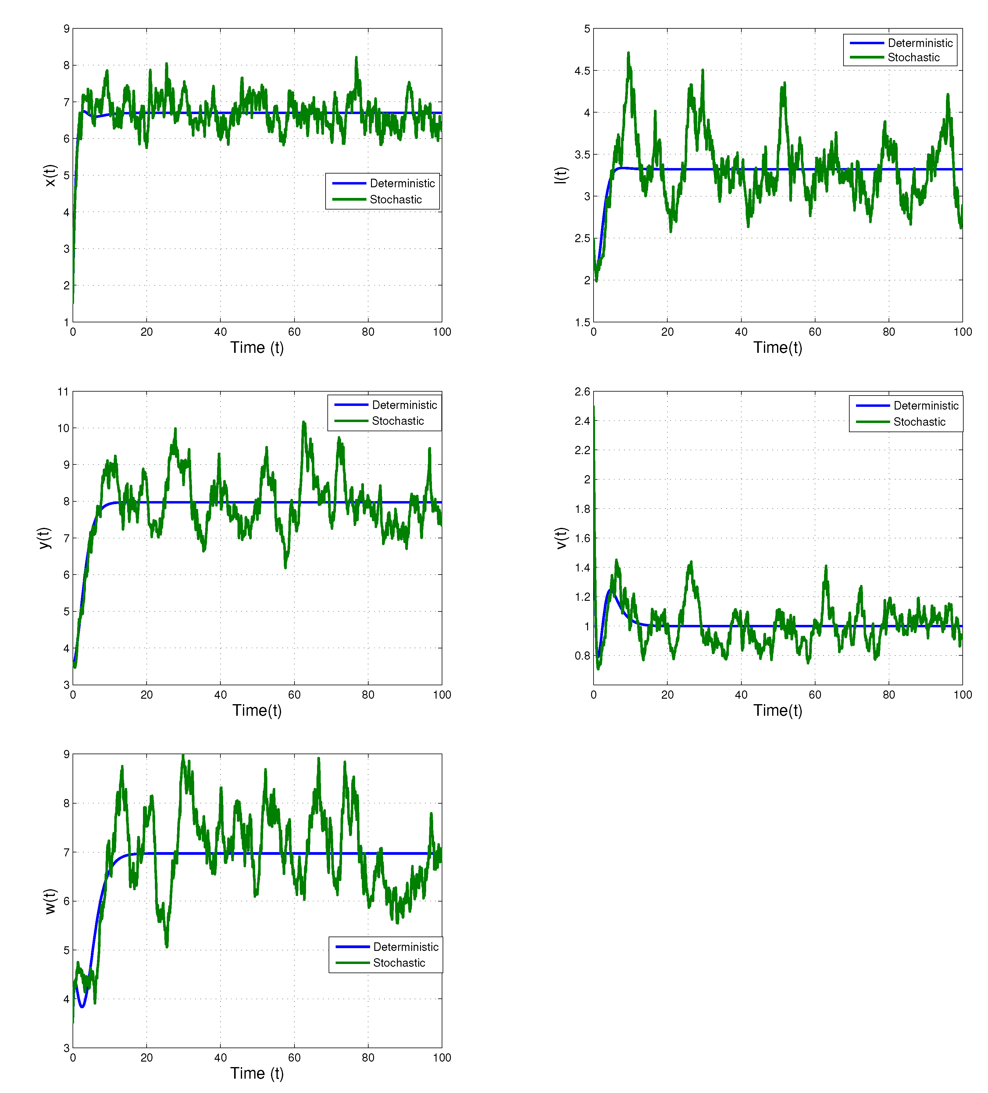
Figure 1. Shows time trajectories of ( x ( t ) , l ( t ) , y ( t ) , v ( t ) , w ( t ) ) of the stochastic model (2) with σ 1 = 0.9 , σ 2 = 0.9 , σ 3 = 0.7 , σ 4 = 0.9 , σ 5 = 0.8 ( R 0 s = 1.5886 > 1 and its corresponding deterministic model. The solution fluctuate randomly with respective stochastic mean, respectively.
Applsci 11 10484 g001
Figure 2. Shows time trajectories of l ( t ) , y ( t ) and v ( t ) of the stochastic model (2) with σ 1 = 3.9 , σ 2 = 3.9 , σ 3 = 3.7 , σ 4 = 3.9 , σ 5 = 3.8 and R ˜ 0 s = 0.5665 < 1 . The stochastic noise is shown to suppress the explosion of population.
Applsci 11 10484 g002
Publisher’s Note: MDPI stays neutral with regard to jurisdictional claims in published maps and institutional affiliations.