Parallel-Structure Deep Learning for Prediction of Remaining Time of Process Instances

Abstract

Event logs generated by Process-Aware Information Systems (PAIS) provide many opportunities for analysis that are expected to help organizations optimize their business processes. The ability to monitor business processes proactively can allow an organization to achieve, maintain or enhance competitiveness in the market. Predictive Business Process Monitoring (PBPM) can provide measures such as the prediction of the remaining time of an ongoing process instance (case) by taking past activities in running process instances into account, as based on the event logs of previously completed process instances. With the prediction provided, we expect that organizations can respond quickly to deviations from the desired process. In the context of the growing popularity of deep learning and the need to utilize heterogeneous representation of data; in this study, we derived a new deep-learning approach that utilizes two types of data representation based on a parallel-structure model, which consists of a convolutional neural network (CNN) and a multi-layer perceptron (MLP) with an embedding layer, to predict the remaining time. Conducting experiments with real-world datasets, we compared our proposed method against the existing deep-learning approach to confirm its utility for the provision of more precise prediction (as indicated by error metrics) relative to the baseline method.

1. Introduction

Nowadays, Process-Aware Information Systems (PAIS) are utilized more and more by companies or organizations to help their operations run better. Concomitantly, the availability of event records, commonly called event logs, is increasing [1]. These event logs, as accompanied by attribute data, can store all information about any activities that have been executed at particular times. The availability of these event logs provides opportunities for the optimization of business processes through data mining and process mining. Data mining analyzes data from event logs without taking business processes into account, in contrast to process mining, which analyzes the overall aspects of all business processes. Process mining techniques enable the extraction of insights contained in event log systems [1]. These insights can help company authorities to improve their business processes. The increasing number of event logs also makes process mining currently the most attractive area in Business Process Management (BPM).

Predictive Business Process Monitoring (PBPM) is a study framework and a branch of process mining that provides predictions of certain measures of interest of ongoing cases based on an event log of past processes [2]. Examples of measures of interest are an activity that will occur next in a running process and the remaining time required by a process for its completion. By acquiring knowledge in advance about a process that is still running, the manager or another person in charge can take action to avoid undesirable situations. One example is a customer’s call to his insurance company to ask about when he can claim his insurance. In this case, he can be given an estimate of the remaining time required by the claim process [3]. Another example is when company authorities can be given early notification of a case that has the potential to have adverse outcomes. Then, they can quickly determine the policies that will be carried out.

Deep learning is a technique that is very popular today due to its ability to solve problems in various fields, especially problems involving images (spatial dependencies) and sequences (Natural Language Processing). Even though deep learning’s basic foundation has long been known [4], it has only recently become very popular with the help of the rapid development of hardware and the discovery of various algorithms that can be relied upon to make neural network (NN) performance much better than in the past [5].

In the context of the growing popularity of deep learning, in this study, we derived and evaluated a new method for solving one of the main problems in PBPM: prediction of the remaining time of process instances based on deep learning and the utilization of the heterogeneous representation of data sources. As evidenced by our experiments, our method could deliver a precise prediction. Additionally, because event logs contain categorical data that are difficult to handle by the FCNN, we propose herein and test in the present study to further strengthen our method, a new encoding technique suitable for event-log-type data and that also utilizes the embedding layer.

1.1. Objectives

As already stated, PBPM is a branch of process mining that aims to provide predictions of measures of interest. Of the several measures of interest that PBPM can provide, in this study, we focused on the prediction of the remaining time needed by a running case to complete. Our study’s expected contributions to the field of PBPM research are as follows:

• Development of an NN architecture that incorporates two models, a convolutional neural network (CNN) and a multi-layer perceptron with data-aware entity embedding (MLP + DAEE), and the proposal of a new method of encoding as applied to event-log-type data;
• Improvement of the accuracy of a deep-learning-based method for the prediction of the remaining time of an ongoing case problem, as confirmed by comparing our method with another deep-learning method used as a baseline method;
• Experimental demonstration that the utilization of chart image representation, specifically the inter-case dependency feature contained therein, can increase the accuracy over the remaining time of the ongoing process prediction problem;
• Provision, to PBPM, of a functional solution in the form of an introduced new deep-learning-based method that does not use a recurrent NN. (To date, all deep-learning-based methods use a recurrent NN.)

Our research was inspired by various other studies, which we will explain in the literature review section (see Section 2 below).

1.2. Definitions and Problem Statement

Here, we provide the definitions and notations used in this paper. The following definitions are the general ones used in the field of process mining [1], with our added definition of a set of prefixes (SOP).

• Definition 2.1.1 (Event). An event is a tuple denoted $e=\left(a,c,t,d_1,d_2,\dots ,d_m\right),$ where $a$ is the activity of the process associated with the event, $a\in A$, while $A$ is a finite set of process activities, $c$ is the case identifier, $c\in C$, $C$ is a set of all case identifiers, $t$ is the timestamp of the event, $t\in T$, $T$ is the time domain, $d_1,d_2,\dots ,d_m$ is a list of other attributes of the event, $d_i\in D_i$, and $D_i$ is a set of all possible values of attribute- $i$. The event universe is denoted $\mathcal{E}$. At each event $e,$ we also define the mapping functions: ${\pi }_A\left(e\right)=a$, ${\pi }_C\left(e\right)=c$, ${\pi }_T\left(e\right)=t$, ${\pi }_{D_i}\left(e\right)=d_i$ where $1\le i\le m$, $m=\left|D\right|$.
• Definition 2.1.2 (Case). A case is a finite sequence of events denoted $\sigma =\left(e_1,e_2,\dots ,e_n\right)\in {\mathcal{E}}^{*}$, where ${\mathcal{E}}^{*}$ is the set of all possible sequences over $\mathcal{E}$, $\left|\sigma \right|=n$, ${\pi }_T\left({\sigma }_i\right)\le {\pi }_T\left({\sigma }_{i+1}\right)$, and $\sigma \left(i\right)$ is the event in case $\sigma$ at index $i$. An ongoing case is a prefix case of length $l\left(l\le n\right)$, denoted ${\sigma }^l=\left(e_1,e_2,\dots ,e_l\right)$.
• Definition 2.1.3 (Event log). An event log is a set of $K$-sized cases, denoted $L=\left\{{\sigma }_i:i=1,\dots ,K\right\},$ such that each event appears at most once in the event log. So, we can write the $i$th case of length $n_i$ as ${\sigma }_i=\left(e_i^1,e_i^2,\dots ,e_i^{n_i}\right)$.
• Definition 2.1.4 (Set of prefixes). A set of prefixes is a converted event log of $N$-size, where $N={{\displaystyle \sum }}_{i=1}^K\left|{\sigma }_i\right|$, which contains the prefixes and other essential properties of all events as tuples, denoted $SOP=\left\{p_k:k=1,\dots ,N\right\}$, with $p=\left(rt,et,pr{e}_{act},pr{e}_{att},t,c\right)$, where $rt$ is the remaining time of a prefix case, $rt\in {ℝ}^{0+}$, $et$ is the elapsed time of a prefix case, $et\in {ℝ}^{0+}$, $pr{e}_{act}$ is the tuple of a prefix of activities, i.e., $\left(a_1,a_2,\dots ,a_l\right), l\le \left|\sigma \right|$, $pr{e}_{att}$ is the tuple of a prefix of attributes, i.e., $\left(d_{1,1},d_{1,2},\dots ,d_{\left|D\right|,l}\right),l\le \left|\sigma \right|$, $t$ is the timestamp of the last event in the prefix case, while $c$ is the case identifier of the prefix case, $t\in T$, $c\in C$. We also define the mapping functions ${\phi }_C\left(p_k\right)$ and ${\phi }_T\left(p_k\right)$ that return $c$ and $t$ respectively at the $k$th $p$.

The problem we are dealing with in this paper is a supervised learning problem, namely the estimation of the remaining time $rt$ of an ongoing business process instance. The objective is to minimize the risk function; we chose the Mean Absolute Error (MAE) over the test set.

2. Related Work

Predictive Business Process Monitoring (PBPM) is a category of process mining that aims to predict a so-called Measure of Interest (MOI) from a process that is still running (incomplete) by utilizing past event logs data consisting of completed processes [2]. Based on the type of output, we can divide PBPM research into several types. The first is research that focuses on predicting all things relating to the time of a process, be it delay, remaining time, or deadline violation. The second is research that focuses on predicting the output of a process, such as whether the process is a normal process or an abnormal process, so that violation can be predicted and prevented as early as possible. The third is research that focuses on predicting succeeding events, such as what activity will occur in those events or what resources will be involved in them. In addition to the research that focuses on types of outcomes, there is also research that focuses on the problem of the optimization of the hyperparameters of the model used. In this subsection, we will discuss the related research as sorted by the time of publication.

The first research relevant to time prediction, especially remaining-time prediction, is the work of van Dongen et al. [6]. Their proposed method uses, as the baseline, non-parametric regression and only the remaining time average those processes have at a given time. The work by van der Aalst et al. [3] is the first to utilize process mining techniques to predict time-related MOI. The authors demonstrate that we can evolve the discovered process model by utilizing a transition system to predict the remaining time of ongoing processes. They also introduced several types of abstraction techniques that could be applied to balance situations of “overfitting” or “underfitting.” To make the model aware of the context in predicting processing time, Folino et al. [7] took advantage of contextual features such as availability of resources and dependence on other attributes. Maggi et al. [2] extended the work of Folino et al. [7] and formalized the problem of PBPM in general.

Leontjeva et al. [8] proposed a method that considers the attribute data loaded by the event rather than just the sequence of activities (simple symbolic sequence) to predict the most probable outcome (positive or negative) of a running process. For their method’s machine-learning model, they used Random Forest. The Queuing Theory proposed by Senderovich et al. [9] predicts a delay in an ongoing process. As in van der Aalst et al. [3], the authors also used annotated transition systems in this prediction task. Besides the work of Maggi et al. [2], de Leoni et al. [10] also proposed a general framework that correlates processes in the event log for predictive purposes. However, the proposed method cannot handle the feature explosion problem that will arise due to the lack of a feature space reduction mechanism. In machine learning, there is the “no free lunch theorem,” whereby a particular model with a hyperparameter configuration is excellent in a specific dataset but awful in another. For that reason, the configuration of the hyperparameters needs to be optimized and adjusted to the specific problem and the dataset encountered. Therefore, Francescomarino et al. [11] proposed a framework that provides an automatic mechanism for optimizing the hyperparameter model used in the area of PBPM.

A solution using deep learning was first proposed by Evermann et al. [12] Their deep-learning architecture consists of two hidden recurrent neural networks (RNN) layers using long short-term memory (LSTM) cells. Tax et al. [13] also used the LSTM architecture. This model is more general because it can predict multiple objectives at once, such as time-related properties, case outcomes, and future event(s). The same model was proposed by Navarin et al. in the same year. Even though it focuses only on one type of prediction—that is, remaining-time prediction—it considers the data attributes attached to the event. LSTM is popularly used in time series prediction problems. However, the use of other types of Neural Networks is no less popular, such as the Autoregressive Network method developed by Bai et al. [14] The research from which we derived the most inspiration is that of Senderovich et al. Their solution focuses on the feature engineering process, which seeks to capture inter-case dependency features, as inspired by processes that run concurrently and access the same resource. Instead of manually performing feature engineering, we can obtain the inter-case dependency by utilizing chart images to predict the remaining time of the ongoing process, which is one of the main focuses of our research. In addition to research focusing on optimization of the hyperparameters mentioned earlier, the same researchers, Francescomarino et al., developed and updated their solutions by using one of the famous evolutionary algorithms, the Genetic Algorithm, an algorithm that mimics the evolutionary process.

In Table 1, for ease of comparison, we summarize some of the related work on PBPM research. Of all the related work that we show, we focus on the problem of remaining-time prediction. We also focus on the latest research, narrowing down the literature to only three studies: those of Tax et al. [13], Navarin et al. [15], and Senderovich et al. [9]. The method by Tax et al. [13] has several problems, such as the amount of time required for the test process and the lack of consideration of data attributes. These issues were handled by Navarin et al. Senderovich et al. [16,17] introduced the concept of inter-case dependencies that can be obtained manually from the feature engineering process. This method inspired us to propose a new method that utilizes deep learning and chart images to capture inter-case dependencies automatically. Thus, we expected our method to outperform the existing deep-learning method, namely data-aware LSTM (DA-LSTM) by Navarin et al. [15], which does not consider inter-case dependencies. Besides that, DA-LSTM also requires a significantly long time to be trained. One of the reasons is that it employs one-hot encoding, with the consequence that the dimensions of the encoding result are enormous, thus rendering it slow to train. Our proposed method also handles these issues.

Table 1. Summary of research in PBPM.

Author	Method	Objective
van Dongen, Crooy and van der Aalst (2008) [6]	Non-parametric Regression technique	Predicting the remaining time
van der Aalst, Schonenberg and Song (2011) [3]	Annotated Transition Systems	Predicting the remaining time
Folino, Guarascio and Pontieri (2012) [7]	Predictive Clustering Tree	Predicting the remaining time
Maggi et al. (2014) [2]	Decision Trees	Predicting the Linear Temporal Logic rules
Leontjeva et al. (2015) [8]	HMM and Random Forest	Predicting the outcome
Senderovich et al. (2015) [9]	Queueing theory	Predicting the delays
Francescomarino et al. (2016)	Clustering and Hyperparameters Optimization	Predicting the Linear Temporal Logic rules
Evermann, Rehse and Fettke (2017) [12]	Deep learning, LSTM	Predicting the next event
Tax et al. (2017) [13]	Deep learning, LSTM	Predicting the remaining time, the outcome, and the next event
Navarin et al. (2017) [15]	Deep learning, Data-Aware LSTM	Predicting the remaining time
Senderovich et al. (2017) [16]	Feature Engineering	Predicting the remaining time
Francescomarino et al. (2018) [11]	Genetic Algorithm	Optimizing the hyperparameters

3. Proposed Method

3.1. Framework

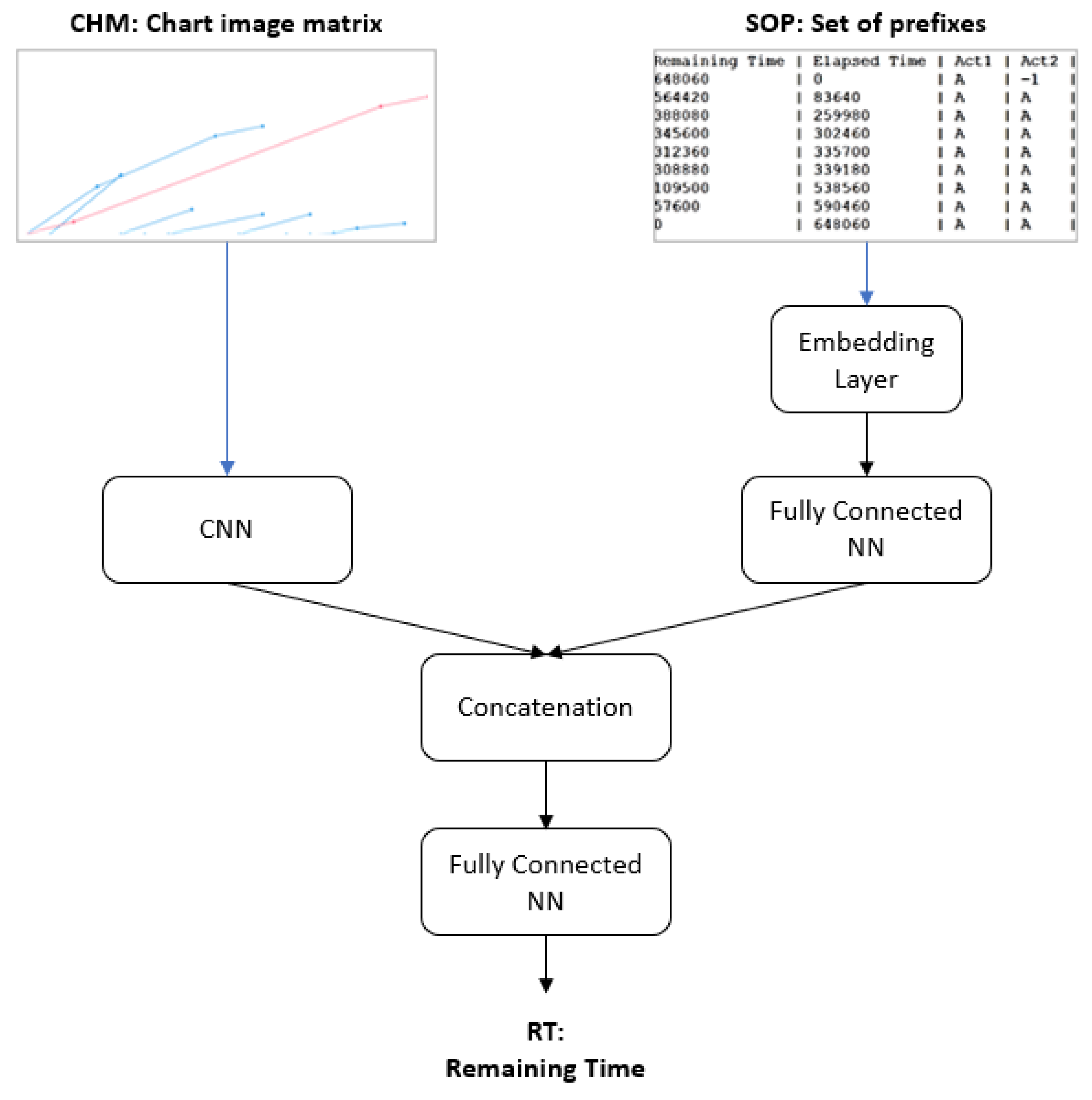
In this subsection, we provide a general description of the framework of our proposed deep-learning model. The problem we were trying to solve in this study was the remaining time of the ongoing process; that is, given all of the features related to an ongoing process, such as the elapsed time, the prefix of activities, and all other attributes, we would like to predict how much time remains for completion of the process. We employed the MAE metric to quantify how much error we incur against the actual values. Our model has a parallel structure consisting of a CNN and an MLP with data-aware entity embedding (MLP + DAEE), as illustrated in Figure 1.

Figure 1. The general framework of the proposed deep-learning model.

The MLP + DAEE part will handle the sequence of categorical variables, while the CNN part will handle image data. A parallel structure is usually used to handle heterogeneous data or when it is expected that more than one type of feature will be extracted from the same data. Our parallel structure is similar to that of the method proposed by Yao et al. [18], which consists of CNN and RNN to classify hematoxylin–eosin-stained breast biopsy images into four classes (normal tissues, benign lesions, in situ carcinomas, and invasive carcinomas). This type of structure is different from the hybrid models used in general, which are usually in-series structures wherein the previous model’s output is used as input to the next model. This was the case in the research conducted by Zhang et al. [19] for the prediction of roll motion in unmanned surface vehicles: they combined two models, CNN and LSTM, using the output of CNN as the input of LSTM. A similar method was proposed by Zheng et al. [20] for the automatic diagnosis of arrhythmias. Le et al. [21] proposed the same architecture to predict electricity consumption, but in place of ordinary LSTM, they used Bi-directional LSTM. Shi et al. [22] developed a parallel deep network combined with data decomposition on a non-stationary time series problem.

3.2. Data Preprocessing

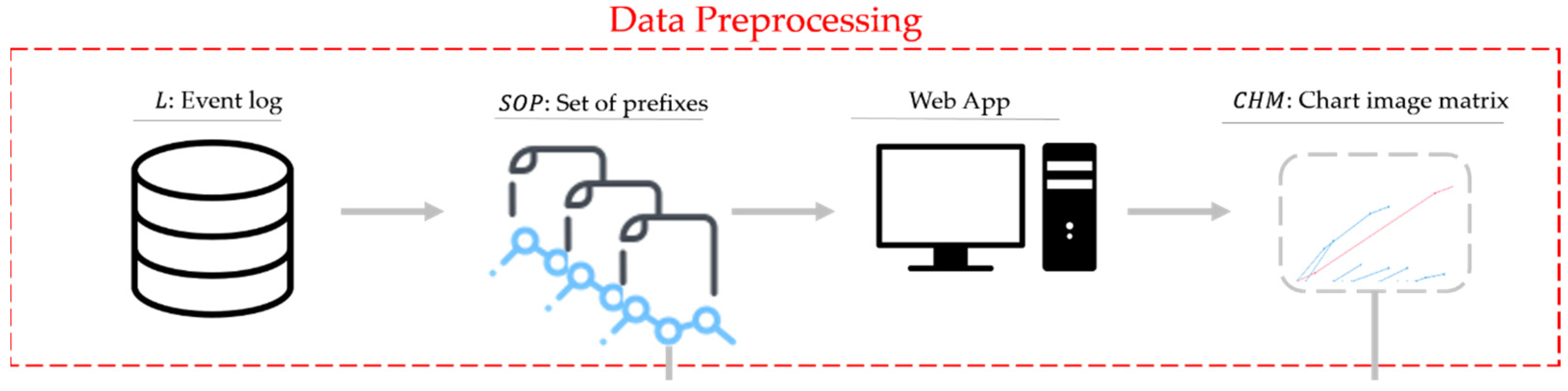
Data preprocessing is a step that must be fulfilled before the data are ready to be used by the model during training. As shown in Figure 1, our proposed method required two types of data as input: the data features forwarded to the Embedding layer, which we call a set of prefixes (SOP), and chart image data, which will be forwarded to the CNN part. Both inputs were originally generated from event logs, as shown in Figure 2. The details of each data generation will be discussed in the following subsections.

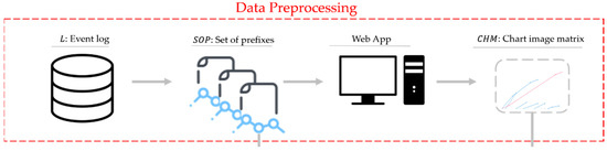
Figure 2. Data preprocessing.

3.2.1. Event Logs to Set of Prefixes (SOP)

For the first type, we convert event logs to an $\mathrm{SOP}$, to which, at each observed event, prefixes are added according to the case of that event. From this process, we also obtain continuous variables, which is to say, the remaining time and elapsed time that the case has. The remaining time itself is a continuous variable that will be the target of prediction.

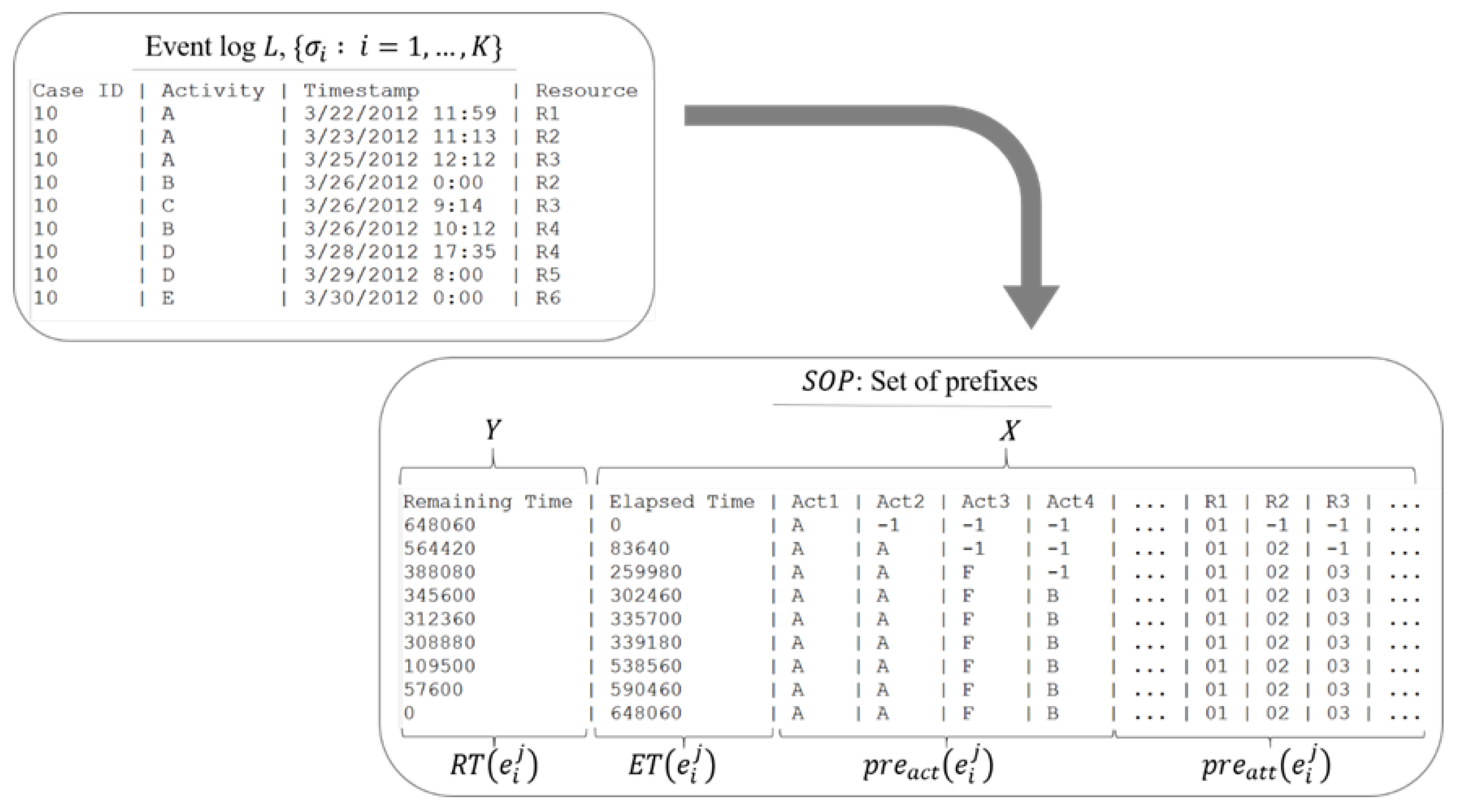
Figure 3 provides an overview of the SOPs obtained from event logs. The process takes event logs with their corresponding fields as input and produces an SOP with the target variable (i.e., the remaining time of an ongoing case), which is our measure of interest, as the output. This preprocessing is commonly used for prediction problems with sequence data, as in Senderovich et al. [16]. We append all its corresponding event sequences for every event in the event log; it can also be called its history. Not only its activities sequence but also all the resources sequence.

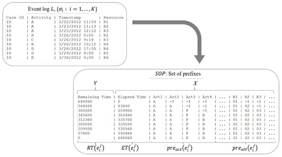
Figure 3. Conversion of the event log to set of prefixes (SOP).

3.2.2. Convert the Set of Prefixes (SOP) to Chart Image

The second input type is the image data. We obtained the image data from the elapsed time of each observed case and all concurrent cases from the start of the observed case begin, which exists in the SOP. The image data are displayed using the Django framework on the backend, which is a python-based web development framework [23], while the chart image on the frontend is rendered using the JavaScript library, Dygraphs [24]. In the case of the chart image displayed on the frontend, the browser is captured using the html2canvas and is sent back to the server. The generated chart images should be clean from unnecessary information in the chart and resized without eliminating essential features in the data to make training lighter and faster, as illustrated in Figure 4. In the conversion process from SOP to chart image data, we obtain the SOP of a given event id (IDX) as an input and convert it to an image. In the prediction task, the use of chart images is still infrequent. With the growing popularity of deep learning, especially in image analysis, there is also a growing need to utilize image data that has previously been ignored, including chart images usually displayed in applications such as dashboard apps and reports. We found two recent reports that proposed the use of chart images. The first study, conducted by Sim et al. [25], used the LeNet-5 architecture, the most popular CNN architecture of its time, to predict the stock market by focusing only on utilizing a CNN and how to optimize it. To demonstrate the reliability and performance of their proposed method, they compared it with Support Vector Machine (SVM) and FCNN. They also showed that the performance of their model could be optimized by selecting a suitable loss function, dropout probability, and an optimization algorithm. The second study was carried out by Lee et al. [26], who utilized chart images that illustrate the stock market pattern. Their proposed model can yield a profit not only in the US market where the training data used were derived but also in other countries; thus, it can be considered to be general. It uses CNN as a function approximator that maps state representations (chart images) to an action (long, neutral, or short), and also employs the Deep Q Network as an algorithm to enable an agent to learn optimal policies; as such, this model is capable of choosing the action that would yield the maximum cumulative reward in a given state.

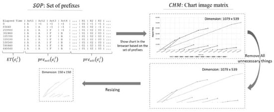
Figure 4. Converting the set of prefixes into a chart image.

In this data representation, information such as intra-case dependencies, how busy the process flow is at a certain time, how many activities occur simultaneously that affect the availability of resources which ultimately affect the time required to complete the process can be obtained. This type of monitoring chart is widely found, by representing the data in this form, we can also use it as a proof of concept that the image from the monitoring diagram can be used even though the construction is still artificial in this paper.

3.3. Network Architecture

A parallel-structure CNN + DAEE architecture consists of two main components, CNN and MLP with data-aware entity embedding (MLP + DAEE). These components are not stacked but are placed in parallel such that there are two streams of input. The MLP + DAEE part is tasked to capture the intrinsic features of categorical variables and the sequence dependencies represented by the SOP; the CNN part is tasked to capture spatial features from chart images, which are expected to represent features that describe the concurrency process of event logs. The purpose of having two components with different functions is to integrate sequence-pattern information and the intrinsic relationships of its categorical variables. Not only that, but the image can also capture inter-case dependencies so that the model can learn patterns better than relying solely on one type of data source. To combine the two streams, we performed an output merger/fusion operation by concatenating the outputs of the two components.

3.3.1. Multi-Layer Perceptron with a Data-Aware Entity-Embedding Layer

The first component of our proposed method is a multi-layer perceptron with a data-aware entity-embedding layer (MLP + DAEE), which accepts an SOP as input. Table 2 describes the details of layer names, layer types, input and output shapes, and their connectivity of the embedding component. Table 3 describes the details of layer names, layer types, input and output shapes, and their connectivity of MLP with the Data-Aware Entity-Embedding component. Note that “n” and “m” in the tables indicate the number of categorical variables and continuous variables, respectively.

Table 2. Input layer for SOP and connectivity of embedding component.

Layer (Type)	Input Shape	Output Shape	Connected to
embed (Embedding)	($\left|D\right|$, 50)	($1, \left|D\right|\times$ 50)	input_dis_1
			input_dis_2
			input_dis_3
			…
			input_dis_n
dense_1 (Dense)	(1)	(1)	input_cont_1
dense_2 (Dense)	(1)	(1)	input_cont_2
dense_3 (Dense)	(1)	(1)	input_cont_3
…	…	…	…
dense_m (Dense)	(1)	(1)	input_cont_m
reshape (Reshape)	($1,\left|D\right|\times$ 50)	($\left|D\right|\times$ 50)	embed[1]
			embed[2]
			embed[3]
			…
			embed[n]

Table 3. Input and output shapes and connectivity of MLP with Data-Aware Entity-Embedding component.

Layer (Type)	Input Shape	Output Shape	Connected to
concatenate_1 (Concatenate)	(1), (1), (1), … (1) ($\left|D\right|\times$ 50), ($\left|D\right|\times$ 50), ($\left|D\right|\times$ 50), … ($\left|D\right|\times$ 50)	(m $+$ (n $\times \left|D\right|\times$ 50)),	dense_1 dense_2 dense_3 … dense_m reshape[1] reshape[2] reshape[3] … reshape[n]
dense_NN_1	(m $+$ (n $\times \left|D\right|\times$ 50))	(500)	concatenate_1
activation_1 (Activation)	(500)	(500)	dense_NN_1
dropout_1 (Dropout)	(500)	(500)	activation_1
dense_NN_2 (Dense)	(500)	(250)	dropout_1
activation_2 (Activation)	(250)	(250)	dense_NN_2
dropout_2 (Dropout)	(250)	(250)	activation_2
dense_NN_3 (Dense)	(250)	(100)	dropout_2
activation_3 (Activation)	(100)	(100)	dense_NN_3
dropout_3 (Dropout)	(100)	(100)	activation_3
dense_NN_4 (Dense)	(100)	(50)	dropout_3

Rectified linear unit (ReLU) [27] is the most widely used activation function in the world right now due to its simplicity but should be applied only to the hidden layer. For both the MLP + DAEE and CNN components, we use the ReLU as an activation function, except for the output layer, where we use the linear activation function because we are dealing with regression problems. We chose ReLU because of its two significant advantages. The first is its ability to reduce the likelihood of gradients to vanish because of its constant gradient growth, unlike the case with sigmoid, where the gradient value gets smaller. The constant gradient in ReLU also causes the learning process of the network to be faster. The second advantage is sparsity because it limits its value to no less than zero, unlike the case with sigmoid, which produces non-zero values, thereby causing dense representation.

A deep NN that is trained on relatively few datasets tends to overfit on training data easily. Generalization error increases due to overfitting. We adopted Dropout [28] for several hidden layers of our network architecture to help to cope with the overfitting problem. As with other hyperparameters in deep learning, the dropout percentage rate (which represents the percentage of neurons that will be dropped out) is also chosen based on trial-and-error experiments in general.

Because the problem we were dealing with in this study is a regression problem, the suitable loss function to be used in the output layer was a choice between Root Mean Squared Error (RMSE) and MAE. We chose MAE because it is more robust to outliers [29]. MAE is obtained from the average of the absolute difference between the actual and predicted values.

Dealing with categorical variables in machine learning is challenging. One known method in machine learning for treating categorical variables is to encode them into integer labels. However, that is insufficient because our machine-learning model will assume that a higher label number has a more significant influence than a lower label number. Therefore, we need an encoding method that assigns equal weight to categorical variables. Thus, some labels do not have a higher weight than other labels. This encoding is known as one-hot encoding. These result variables are also called dummy variables. One feature will be broken down into as many cardinals as the feature, with only one of them having a value of one, all of the others having a value of zero. The one-hot encoding technique has some disadvantages, such that if a feature has variables with a high cardinality level, the number of binary columns produced will be vast, and the dataset will become very sparse or have very high dimensions as a result. Not only that, but the values that are similar to each other also are not placed close together in dimensional space. The result is that the intrinsic properties of the feature are eliminated. One approach that can overcome these problems is a technique known as entity embedding [30]. By using the entity-embedding encoding technique, values that have similar intrinsic properties will be placed close together in space. Additionally, memory usage will be reduced since the dimensions of features are smaller than those of one-hot encoding.

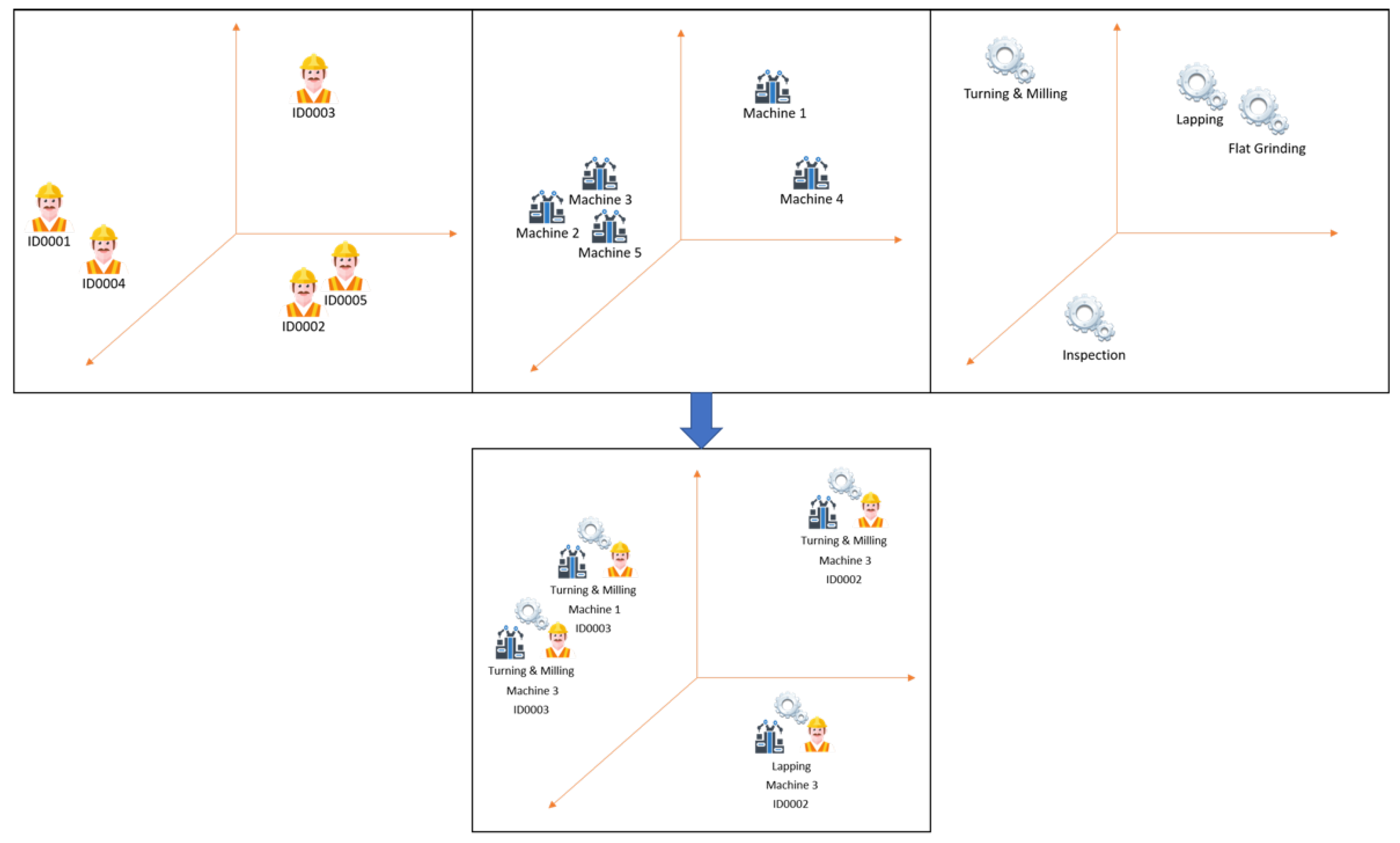
We propose a better encoding method that is suitable for event-log-type data. Instead of encoding each entity as one variable (entity embedding), we build up a fixed-size vector consisting of all different entities. We call this method Data-Aware Entity Embedding (DAEE). It is expected to decrease memory by $n$ times, where $n$ is the number of different types of entities. Based on our domain knowledge of the manufacturing process, a particular activity can experience differences in performance depending on the resources that run it. So, we can obtain a better encoding representation if we do not treat each entity as one variable but instead attach it to others (e.g., attach the resource to the activity). The expected outcome vectors of the embedding are shown in Figure 5. For example, in a typical embedding entity, Machine-1, Operator-ID0001, and Inspection-activity will each be represented as a single vector of its own. In DAEE, Inspection activity will be attached with any data associated with it before being represented as an embedding. For example, Inspection-activity performed by Operator-ID0001 on Machine-1 will be represented as a vector of its own. The process of attaching the data associated to certain activities is shown in Algorithm 1.

Algorithm 1. DAEE Build-Up from SOP

Input: $L$: Event log, $\left\{{\sigma }_i:i=1,\dots ,K\right\}$, $SOP$: Set of prefixes, $\left\{p_i:i=1,\dots ,N\right\}$, sorted by its ${\phi }_T$ Output: $DAE$: Data-Aware Events Begin 1: $max\_length\leftarrow max\left(\left|{\sigma }_1\right|,\left|{\sigma }_2\right|,\dots ,\left|{\sigma }_K\right|\right)$ 2: $DAE\leftarrow \varnothing$ 3: for$i\leftarrow 1\dots N$ do 4:  $row\leftarrow \varnothing$ 5:  for$j\leftarrow 1\dots max\_length$ do 6:    $tuple\leftarrow \varnothing$ 7:    $tuple\leftarrow tuple\parallel {\rho }_{act}\left(i,j\right)$ 8:    for$k\leftarrow 1\dots \left|D\right|$ do 9:      $tuple\leftarrow tuple\parallel {\rho }_{att}\left(i,j,k\right)$ 10:    end for 11:    $row\leftarrow row\parallel tuple$ 12:  end for 13:  $DAE\leftarrow DAE\parallel row$ 25: return$DAE$ End

Figure 5. Illustration of comparison of vectors of entity embedding (top) with those of DAEE (bottom) in multi-dimensional space.

Algorithm 1 shows how to build up the fixed-size vector data-aware events from the SOP. We now introduce some functions: ${\rho }_{act}$ returns the activity at row $i$ and at the $j$-th event in the SOP, while ${\rho }_{att}$ returns the $k$-th data attribute at row $i$ and at the $j$-th event. It is noted here that data attributes include only the categorical variables, just like in the SOP.

Before the data-aware events input enters the MLP part, it is passed to the embedding layer, where the value of each vector will be updated in line with the training process of the network. The issue of how to determine the number of dimensions in the embedding layer is still being researched [30]. Therefore, we determine it with an arbitrary number, which is high, so that the network can learn a good representation compared with having only a single number, but also not too high, which would cause loss of representation (so that the result would be the just same as that with one-hot encoding). As for the continuous variable input, it is received by precisely one neuron. We concatenate all of the output vectors of the embedding layer and input neurons that handle continuous variables before finally forwarding them to the MLP. We obtained an acceptable performance using this model in comparison with other machine-learning models, such as deep learning with one-hot encoding [31].

In the MLP part, empirically, the deeper (the more the hidden layers of) the network, the better the generalization ability. Therefore, we used four layers heuristically while performing trial and error experiments (also known as the babysitting method) with other options. As for the number of neurons in each hidden layer, there are no fixed rules regarding this determination, but we followed a best practice: the number of neurons in the hidden layer is between the number of neurons in the input layer and that in the output layer, and the number of neurons in the hidden layer that is closer to the output layer is less than the number of neurons in the hidden layer closer to the input layer.

3.3.2. Convolutional Neural Network (CNN)

The second component of our proposed method is a convolutional neural network (CNN). A CNN is one of the NN architectures that is successfully applied to solve image classification problems [32]. An image can be seen as a matrix that contains pixel values. CNN is always the go-to solution when dealing with prediction problems involving images nowadays. Similarly, regarding the problem we are dealing with in this study, to handle the input image, we use CNN as a component of the architecture of our proposed method.

The CNN architecture that we use is similar to AlexNet [32] and was inspired by it. AlexNet, a famous CNN architecture for computer vision problems, consists of blocks of the convolutional and pooling layers. Based on AlexNet, we changed some parts of the structure based on experiments and the trusted rule of thumb to determine the CNN hyperparameters. Layers closer to the input layer learn fewer convolutional filters, while layers closer to the output layer will learn more filters. Table 4 describes the details of layer names, layer types, input and output shapes, and the connectivity of our CNN component.

Table 4. Input and output shapes and connectivity of CNN component.

Layer (Type)	Input Shape	Output Shape	Connected to
input_image (InputLayer)	(150, 150, 3)	(150, 150, 3)
conv2d_1 (Conv2D)	(150, 150, 3)	(150, 150, 32)	input_image
max_pooling2d_1 (MaxPooling2D)	(150, 150, 32)	(75, 75, 32)	conv2d_1
conv2d_2 (Conv2D)	(75, 75, 32)	(75, 75, 64)	max_pooling2d_1
max_pooling2d_2 (MaxPooling2D)	(75, 75, 64)	(37, 37, 64)	conv2d_2
conv2d_3 (Conv2D)	(37, 37, 64)	(37, 37, 96)	max_pooling2d_2
max_pooling2d_3	(37, 37, 96)	(18, 18, 96)	conv2d_3
conv2d_4 (Conv2D)	(18, 18, 96)	(18, 18, 96)	max_pooling2d_3
max_pooling2d_4	(18, 18, 96)	(9, 9, 96)	conv2d_4
flatten_1 (Flatten)	(9, 9, 96)	(7776)	max_pooling2d_4

3.3.3. DAEE and CNN Output Concatenation

As illustrated in Figure 1, the last component of our proposed method is the concatenation of the DAEE and CNN outputs. Concatenation is simply a merging operation that is performed on multiple networks so that the merged result can be an input to another network model. Table 5 summarizes the details of layer names, layer types, and input and output shapes of the fully connected NN to the output layer.

Table 5. Summary of the concatenation of output of MLP with DAEE and CNN for fully connected NN to the output layer.

Layer (Type)	Input Shape	Output Shape	Connected to
concatenate_2 (Concatenate)	(50) (7776)	(7826)	dense_NN_4 flatten_1
dense_NN_5 (Dense)	(7826)	(512)	concatenate_2
dense_NN_6 (Dense)	(512)	(100)	dense_NN_5
dense_NN_7 (Dense)	(100)	(10)	dense_NN_6
dense_NN_8 (Dense)	(10)	(1)	dense_NN_7

4. Experimentation and Results

Our proposed method is implemented using the Python programming language. There is also a web development framework that makes it easy for programmers to create a web application very quickly using Python, namely Django. We use this to create a web application that simulates the chart’s appearance according to the event log at a certain point in time. To render the chart itself in the browser, we use Dygraph, which is a javascript library, to render various graphs quickly and very lightly. We use Keras [33], Python library, with TensorFlow on the backend to implement our deep-learning model. We chose Keras because it makes it easy for us to do fast experimentation and prototyping while preserving its flexibility, and it is also straightforward to set up to run seamlessly on a dedicated Graphics Processing Unit (GPU). In the process of training our deep-learning model, we implemented the Early Stopping technique [34] to control overfitting conditions during the training process. With the help of the validation test, we can stop the training before converging when the validation test loss does not decrease after several epochs, which parameter is called “patience.” For our proposed model, we set it at Patience 50, while for the baseline method, which is based on the LSTM model, we set it at Patience 100. This setting is also based on the trial-and-error experiments we conducted. The LSTM model was set higher because it is slower than our proposed model due to the update weights processed during training. We also adopted Adam [35] as the optimization algorithm. Adam is an adaptive learning rate method that computes individual adaptive learning rates for different parameters. Adam can also be called an optimizer, and as such, it can be said to combine the advantages of two popular predecessor algorithms, namely Root Mean Square Propagation (RMSProp) and Adaptive Gradient Algorithm (AdaGrad).

4.1. Data Description

The event log data that we used to conduct our experiments are public data that we had obtained from a Process Mining site [36]. The data are event logs from a manufacturing process. This dataset has 55 types of activities, 225 cases, and 4542 events, so that, on average, each case has ~20 events. This dataset also provides information on the number of human resources and machine workers involved, 49 and 31, respectively. This dataset is a real-world event log that was compiled from January to March 2012. We chose this dataset because the number of events that can occur in one case is quite large, and there is also information on resources involved in the process, making it suitable for demonstration of our proposed method’s capturing of relationships between processes that occur concurrently; it also involves the same resources, which in fact can affect process performance and ultimately affect the time needed for the process to complete. We show a fragment of this event log in Table 6.

Table 6. Fragment of event log from manufacturing process.

Case ID	Activity	Resource	Timestamp	Work Order Qty	Part Desc.	Worker ID	Report Type	Qty Completed	Qty Rejected	Qty for MRB	Rework
Case 1	Turning & Milling—Machine 4	Machine 4—Turning & Milling	1/29/12 23:24	10	Cable Head	ID4932	S	1	0	0
Case 1	Turning & Milling—Machine 4	Machine 4—Turning & Milling	1/30/12 5:44	10	Cable Head	ID4932	D	1	0	0
Case 1	Turning & Milling—Machine 4	Machine 4—Turning & Milling	1/30/12 6:59	10	Cable Head	ID4167	S	0	0	0
Case 1	Turning & Milling—Machine 4	Machine 4—Turning & Milling	1/30/12 7:21	10	Cable Head	ID4167	D	8	0	0
Case 1	Turning & Milling Q.C.	Quality Check 1	1/31/12 13:20	10	Cable Head	ID4163	D	9	1	0
Case 1	Laser Marking—Machine 7	Machine 7—Laser Marking	2/1/12 8:18	10	Cable Head	ID0998	D	9	0	0
Case 1	Lapping—Machine 1	Machine 1—Lapping	2/14/12 0:00	10	Cable Head	ID4882	D	0	0	0
Case 1	Lapping—Machine 1	Machine 1—Lapping	2/14/12 0:00	10	Cable Head	ID4882	D	0	0	0
Case 1	Lapping—Machine 1	Machine 1—Lapping	2/14/12 9:05	10	Cable Head	ID4882	D	1	0	0
Case 1	Lapping—Machine 1	Machine 1—Lapping	2/14/12 9:05	10	Cable Head	ID4882	D	8	0	0
Case 1	Round Grinding—Machine 3	Machine 3—Round Grinding	2/14/12 9:13	10	Cable Head	ID4445	S	0	0	0
Case 1	Round Grinding—Machine 3	Machine 3—Round Grinding	2/14/12 13:37	10	Cable Head	ID4445	D	9	0	0
Case 1	Final Inspection Q.C.	Quality Check 1	2/16/12 6:59	10	Cable Head	ID4493	D	0	0	0

4.2. Experimental Setup

To demonstrate the reliability and robustness of our proposed method, we used another deep-learning method, proposed by Navarin et al. [15], as the baseline method. This method, called Data-Aware LSTM (DA-LSTM), utilizes the LSTM architecture. Unlike the previous research, which also utilizes LSTM, it considers the attribute data of events. With this method, to determine the number of layers and neurons, we also used trial and error (as we did in our proposed method). If the layers are more than two, the training process will be very long, but the performance will not improve. For that reason, we chose to use two layers. Unlike our model, which uses Adam as its optimizer, Navarin et al. [15] chose to use Nadam as the optimizer of their model. To demonstrate the effect without using a chart image in our model, we also compared it with a model without a CNN component (MLP + EE), which does not receive a chart image as its input. Additionally, to demonstrate the superiority of our method that uses DAEE, we compared it with a model that uses only ordinary embedding (Entity Embedding) to encode each discrete variable unit (CNN + EE). Note that all of the hyperparameters we used in our complete model are the same as this model’s, except for the batch size, which has memory limitations due to the length of the input vector and image input. We summarize the four methods used in the experiment below:

• CNN + DAEE, our full proposed method, consists of a combination of two NN models, CNN and MLP with DAEE;
• CNN + EE, the same model as CNN + DAEE, except that it uses entity embedding as its encoder;
• MLP + EE, which is one part of our proposed method without the CNN model, to show the impact of not utilizing chart images;
• DA-LSTM, the latest method based on deep learning for the prediction of the remaining time of an ongoing process problem.

We adopted the k-fold cross-validation (CV) technique [37] to validate and evaluate the reliability of our model. We chose 5-fold because it was enough to show the consistency of the model and not so much that it becomes time-consuming and very computationally expensive. Before we performed the split, we shuffled the dataset randomly. We used 20% of the dataset as test data and the rest (80%) for training in each iteration. In each of those iterations, the test set did not have the same data as the test in the other iterations. The training data (80%) was divided again into two portions, 70% (56% of the total dataset) for training, and the remaining 30% (24% of the total dataset) for the validation test, which was chosen as part of the dataset used to validate the model during training (to avoid overfitting of the training data). We used the Scikit-Learn library to help with this.

All of the models were trained and validated using a computer with the specifications shown in Table 7.

Table 7. Experimental-environment specifications.

Component	Specification
CPU	Inter(R) Core (TM) i7-7700HQ CPU @ 2.80GHz 2.81 GHz
GPU	NVIDIA GeForce GTX 1050—4.0 GB Dedicated GPU Memory
Memory	16 GB
Operating System	Windows 10

4.3. Results

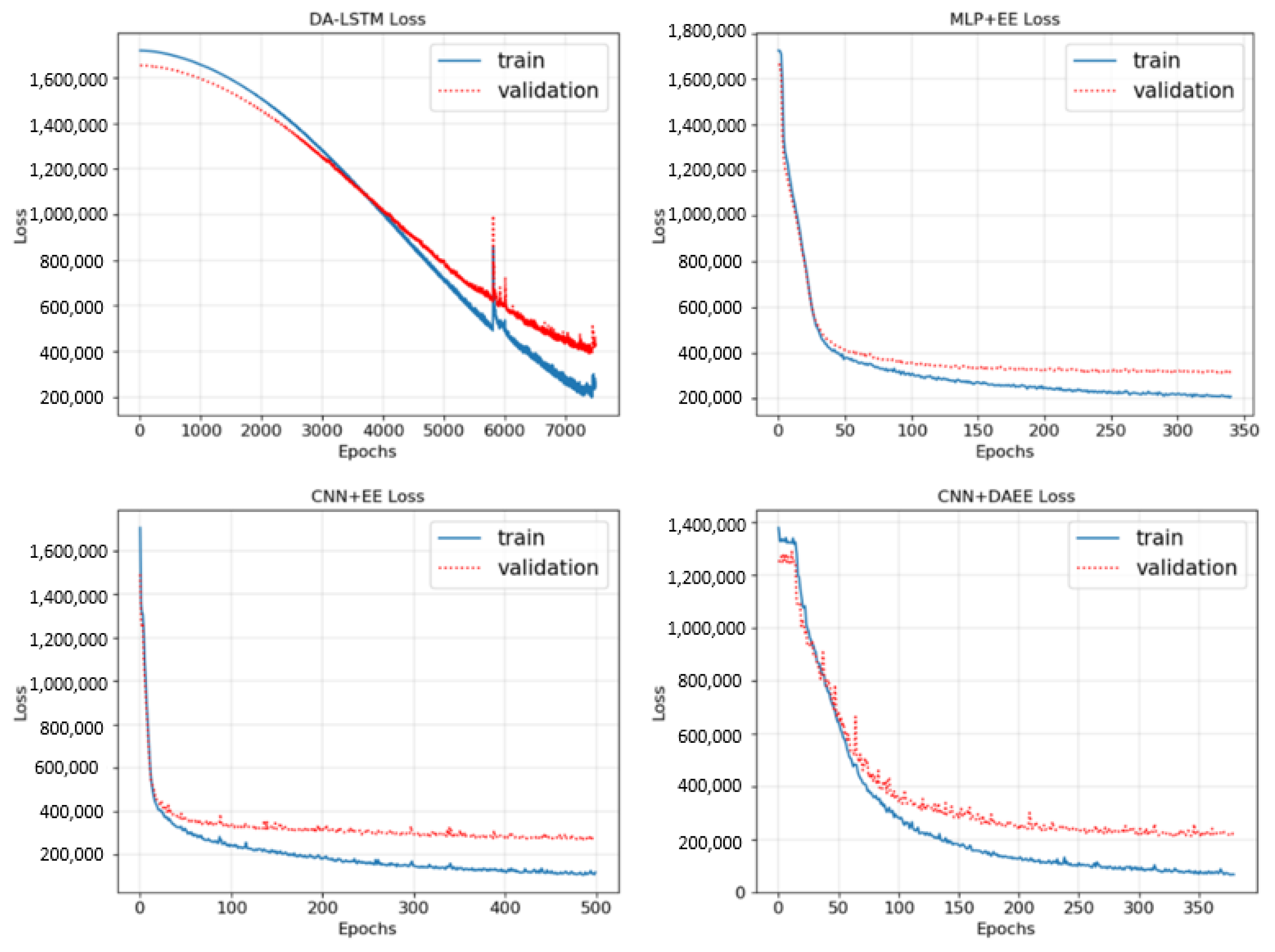
In this subsection, we will discuss the results of the experiments conducted. In Figure 6, we demonstrate the loss (MAE) trend of the training of the four models on one of the iterations of CV.

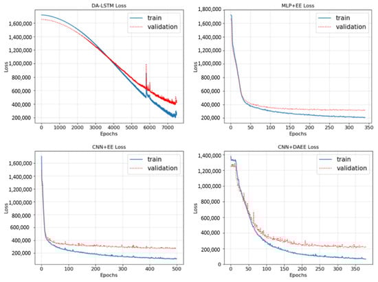
Figure 6. Training and validation loss curves of four models.

We show only one of the five folds, because the pattern is like the other folds, which means that the training process for the five folds can be said to be consistent. MLP + EE and CNN + EE tended to be the same, MLP + EE more quickly experiencing overfitting conditions due to having less input (without chart images), so that we stopped the training process earlier than with CNN + EE or CNN + DAEE. CNN + DAEE experienced a relatively unstable training process at the beginning. The point where the last or best weights are stored is when the validation test reaches the lowest point. Also, as shown in Figure 6, in the graph for DA-LSTM specifically, there is a spike that occurs before returning to stability. Such a spike is a common thing that can happen if we use a batch strategy in the training process.

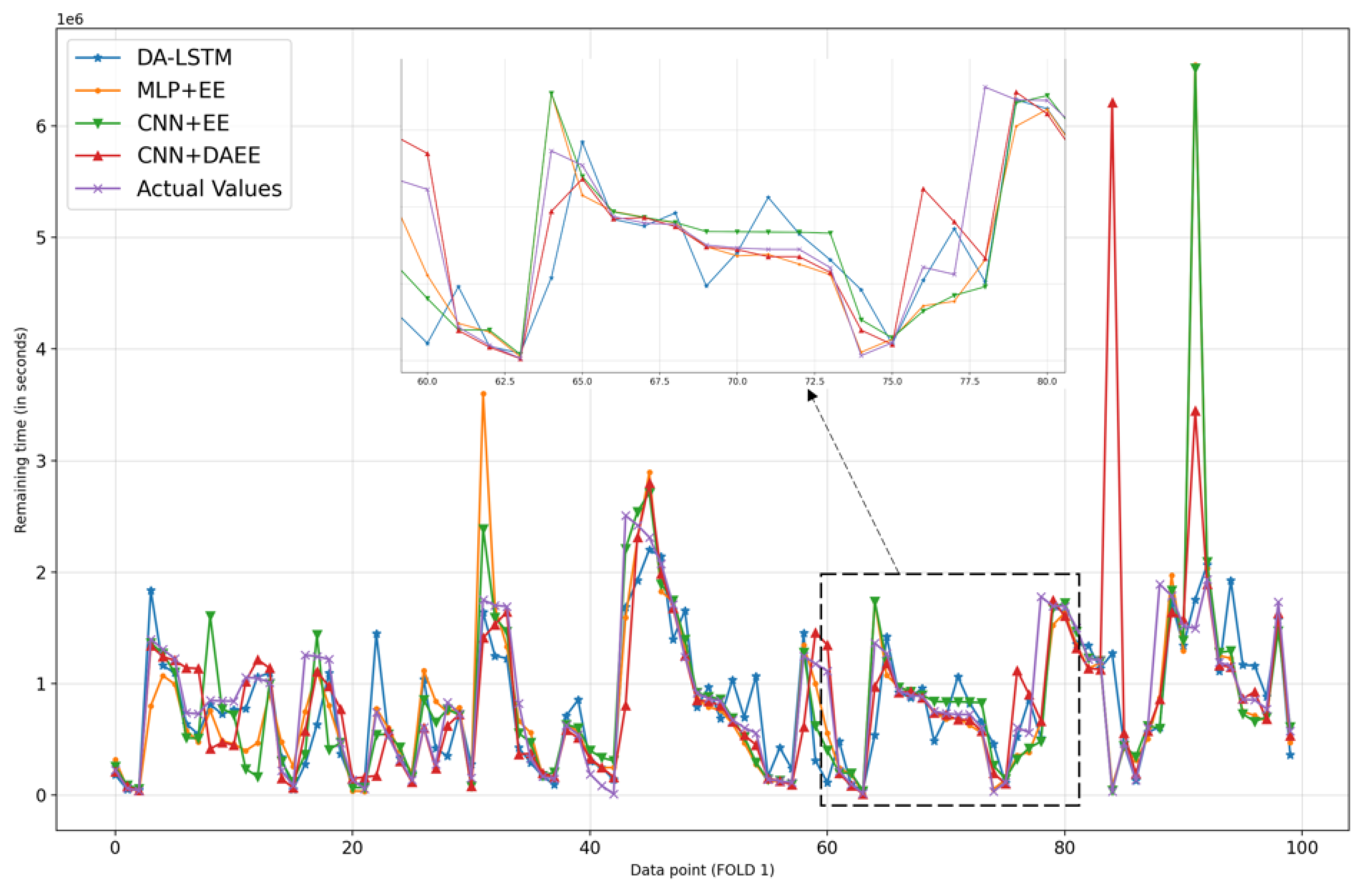
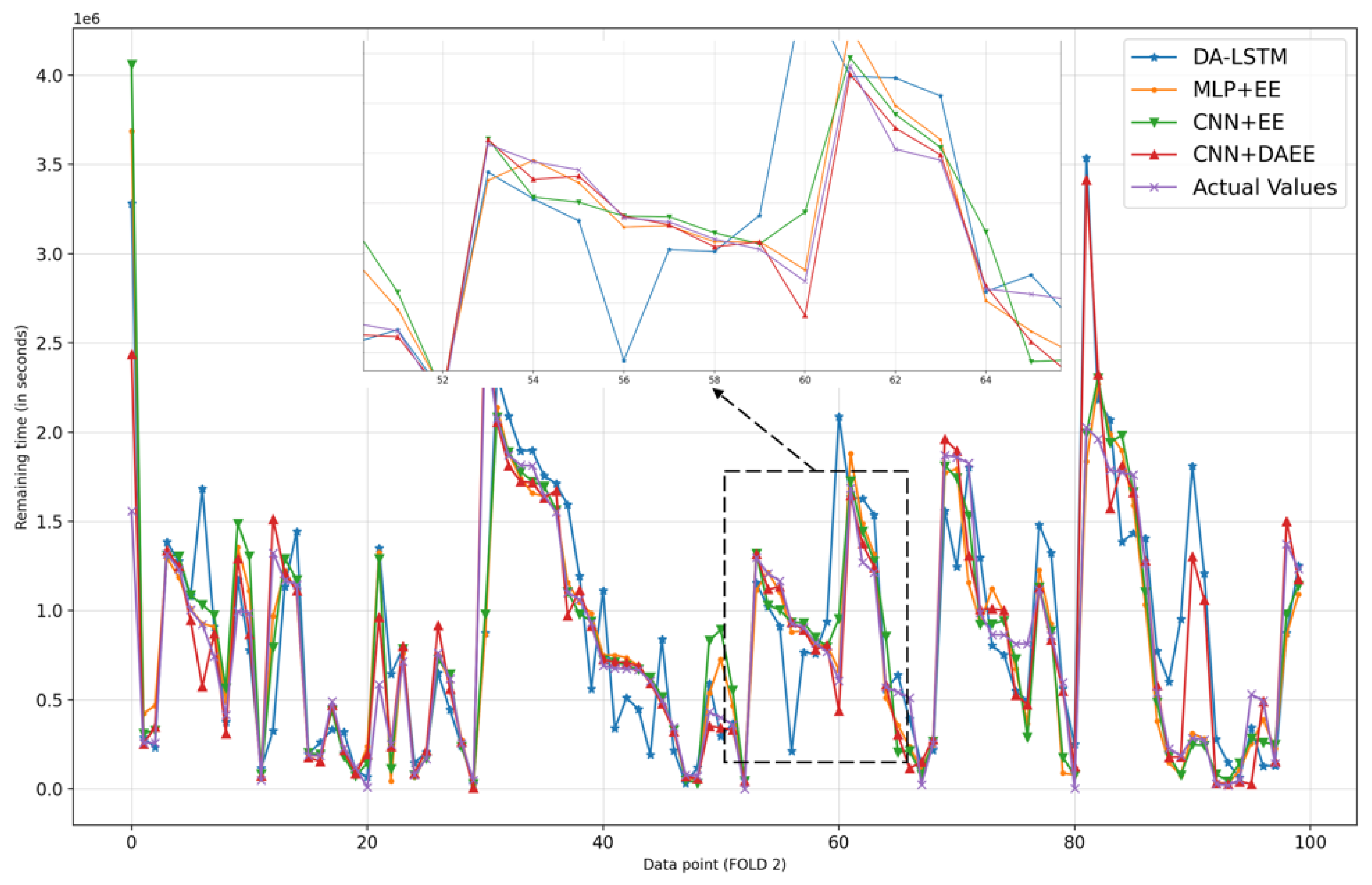
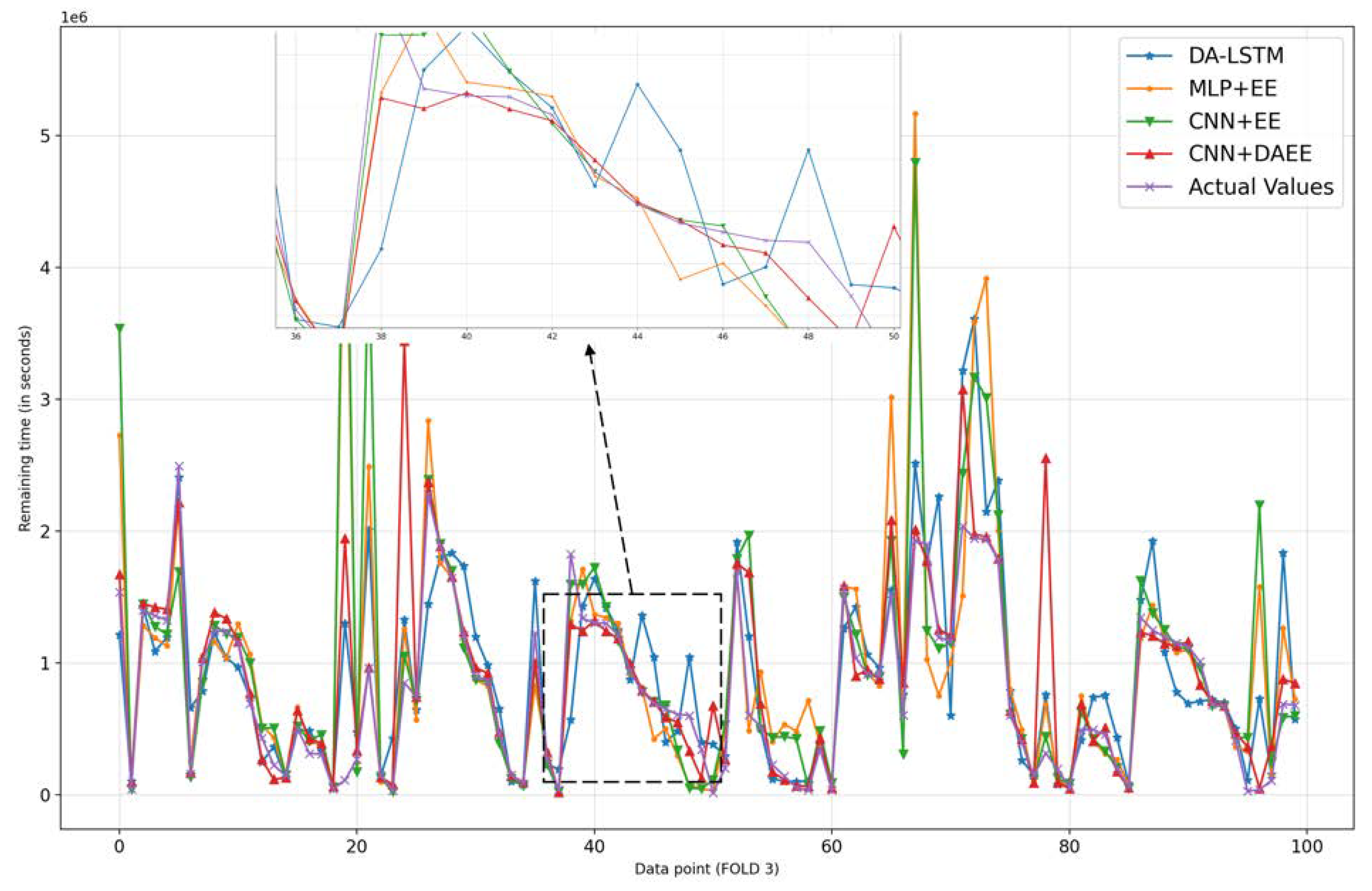
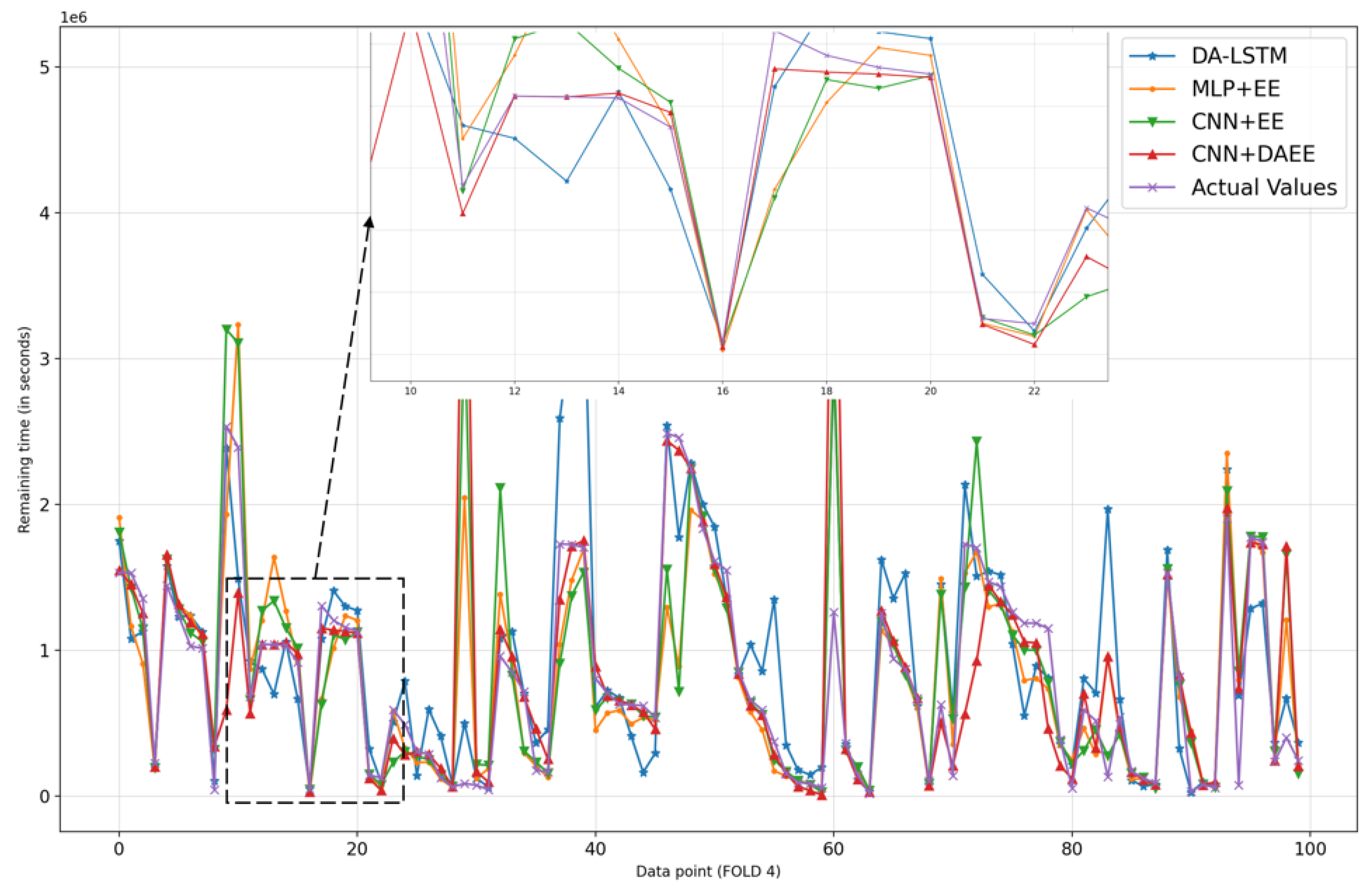
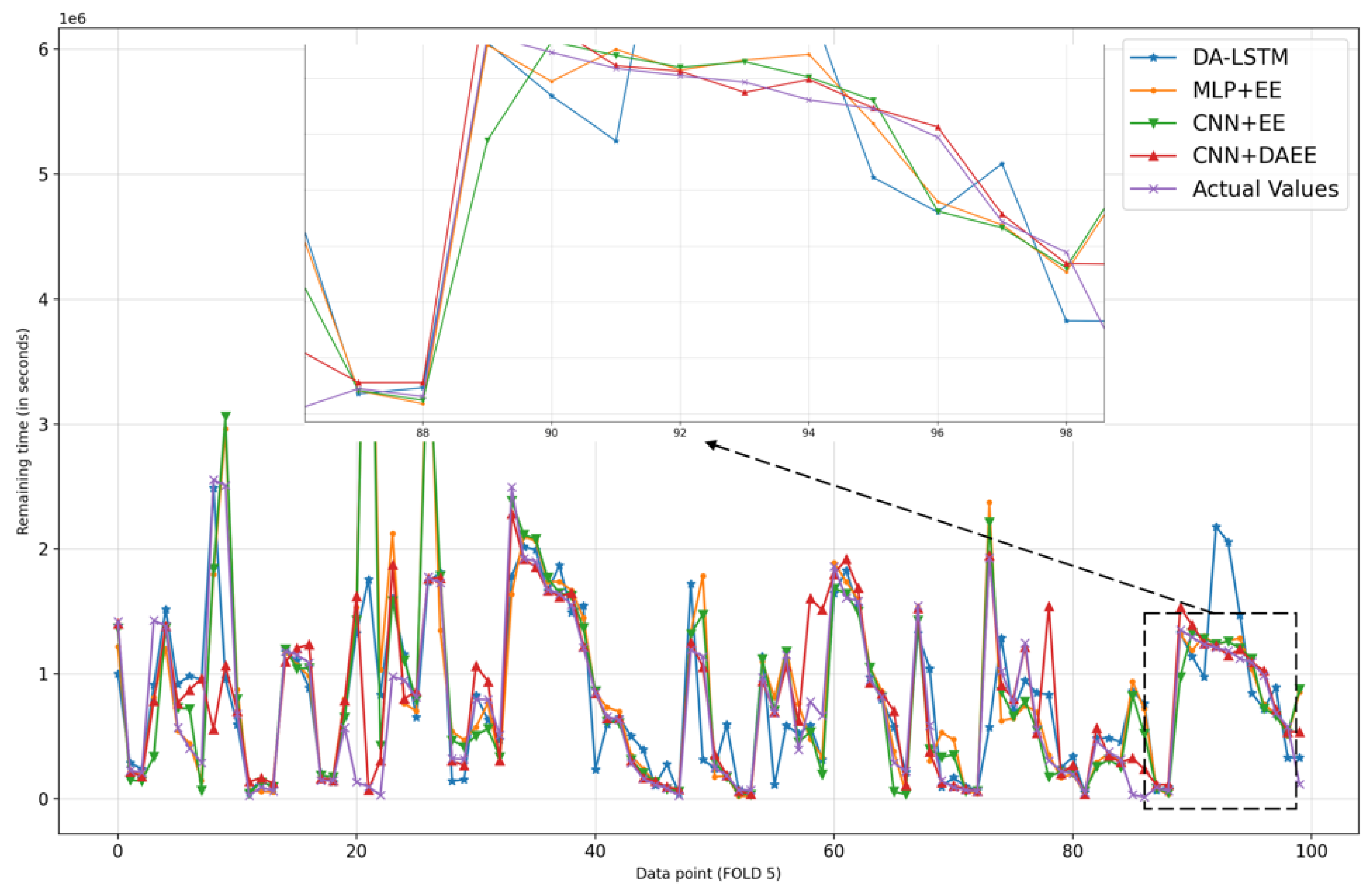
We also show, in Figure 6, Figure 7, Figure 8, Figure 9, Figure 10 and Figure 11, prediction results for all five iterations of CV using the four models. Please note that the graph of the ground truth looks different in each of the four models because the scale is relative to the maximum value of predicted results by each model. We can see from the patterns that the four models provide reasonable predictions. MLP + EE, CNN + EE, and CNN + DAEE tend to have the same prediction results relative to DA-LSTM and to be more accurate, though, at some points, there can be vast differences between actual values and predicted values. For example, in Figure 7, our model considers some values as outliers, and because it optimizes MAE, the outlier is calculated as a minor penalty.

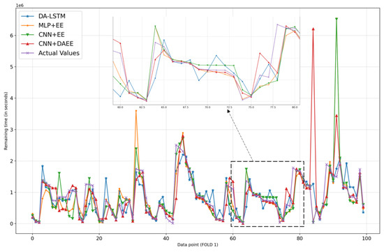
Figure 7. Comparison of results of four models for 100 sample test sets in first iteration of CV.

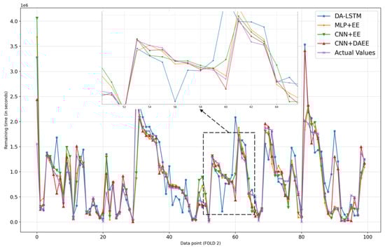
Figure 8. Comparison of results of four models for 100 sample test sets in second iteration of CV.

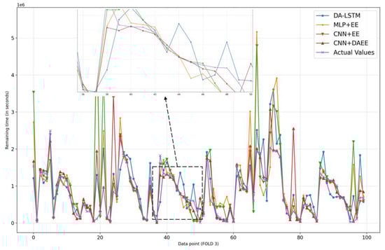
Figure 9. Comparison of results of four models for 100 sample test set in third iteration of CV.

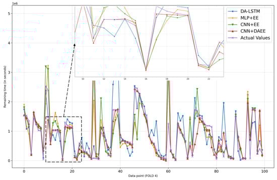
Figure 10. Comparison of results of four models for 100 sample test sets in fourth iteration of CV.

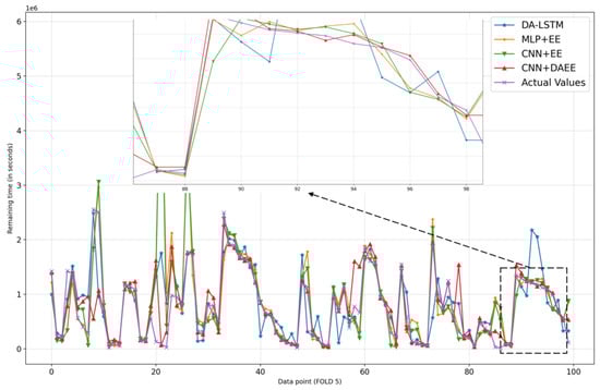
Figure 11. Comparison of results of four models for 100 sample test sets in fifth iteration of CV.

To show the tangible difference of our proposed model in terms of accuracy, we provide a comparison of the errors in MAE and the training time required for each of the four models in Table 8 and Table 9, respectively. We can see that CNN + DAEE outperforms the other three models for all iterations. MLP + EE is superior to both models in terms of training duration, far superior to DA-LSTM, but only slightly superior to CNN + EE and CNN + DAEE because it has the same model structure, except that MLP + EE does not receive chart images as its input and lacks the CNN component. The duration of performance training of CNN + DAEE is slightly superior to that of CNN + EE; this was caused by the length of the vector input generated using DAEE was less than that generated using Entity Embedding.

Table 8. Accuracy (MAE) in units of minutes.

Iteration	MAE (Minutes)
	DA-LSTM	MLP + EE	CNN + EE	CNN + DAEE
1st	5221.646	5362.156	4416.111	3617.575
2nd	4945.532	4973.759	4749.251	3793.084
3rd	7191.880	5578.992	4853.482	3301.337
4th	7176.215	5654.634	4910.471	3641.002
5th	5988.119	5096.931	4935.983	3232.011

Table 9. Training duration in hours: minutes format.

Iteration	Training Duration (Minutes)
	DA-LSTM	MLP + EE	CNN + EE	CNN + DAEE
1st	14:38	01:22	02:31	02:19
2nd	15:16	01:16	02:35	02:03
3rd	15:00	01:16	02:36	02:05
4th	12:12	01:13	02:36	01:39
5th	15:01	01:50	02:39	02:09

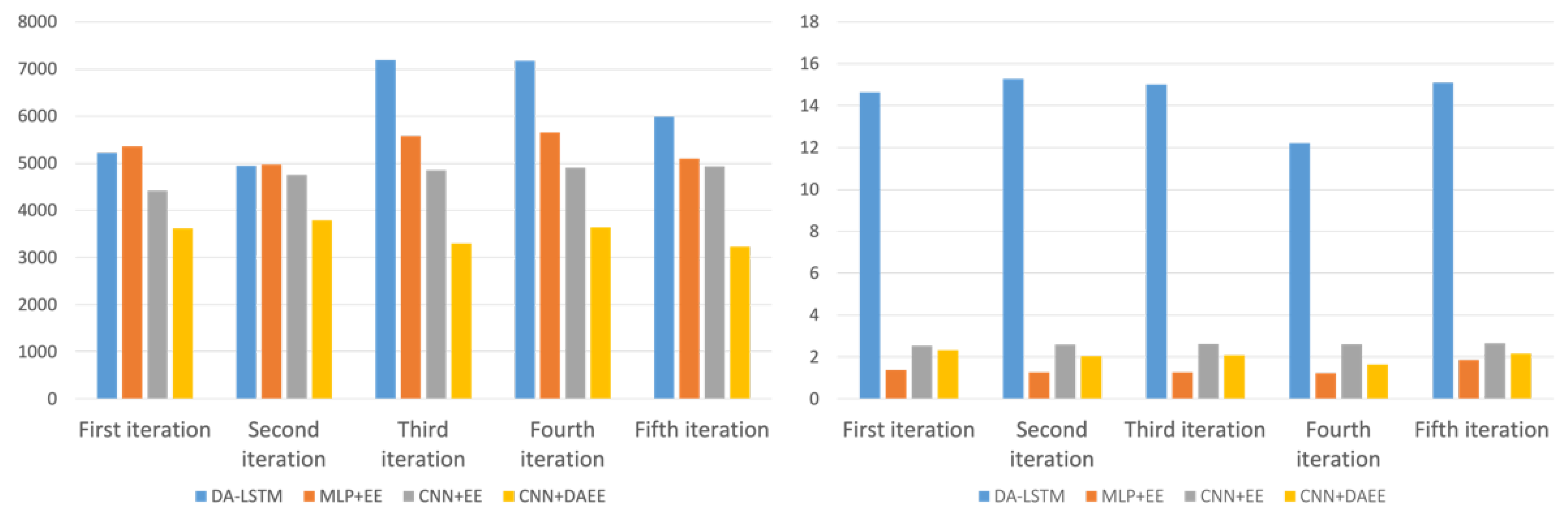
To show the tendency and ratio visually, we also show, in Figure 12’s histograms, a performance comparison in terms of MAE and training duration. There it can be seen that MLP + EE, CNN + EE, and CNN + DAEE are far superior to DA-LSTM in terms of the time needed for training. In terms of accuracy, all four models show a consistent trend across all iterations, CNN + DAEE being the best model.

Figure 12. MAE in units of minutes (left) and training duration in units of hours (right).

We show the average performances of the four models in Table 10. The proposed method (CNN + DAEE) had the best accuracy in predicting the remaining time, which was increased by 42% over that of DA-LSTM, 34% over that of MLP + EE, which does not use chart images as input, and 26% over that of CNN + EE, which uses Entity Embedding as its categorical variable’s encoder. In terms of training duration performance, MLP + EE was about ~14 times more efficient than DA-LSTM but only slightly more efficient than CNN + EE and CNN + DAEE. CNN + EE and CNN + DAEE experienced only a slight decrease in performance in exchange for better accuracy.

Table 10. Mean training duration and MAE in units of minutes across five iterations of CV.

	DA-LSTM	MLP + EE	CNN + EE	CNN + DAEE
MAE	6104.678	5333.294	4773.060	3517.002
Training duration	861.400	83.600	155.400	123.000

5. Discussion and Conclusions

In this study, we derived and evaluated a new approach, namely a parallel-structure deep-learning model named CNN + DAEE, for application in the PBPM field, particularly for predicting the remaining time of an ongoing process (case) using chart images. Our proposed method produced more precise accuracy relative to the baseline method (DA-LSTM), as indicated by the MAE metric and proven and demonstrated by empirical experiments using real-world datasets. We showed that the model’s performance indeed proves to be better with the addition of another representation type of data. In terms of the performance duration of the training, our proposed method is far more practical; in fact, seven times better than the baseline method (DA-LSTM). In our method, we use only an MLP and SOP as input to capture sequence dependencies from data and handle categorical variables very well using embedding rather than the usual and proven model in the sequence problem, namely LSTM. One major consideration is the length of time required for training. MLP proved to be reasonably reliable compared with LSTM in this study, and its performance was improved by combining it with another model (CNN). By adding another representation type of data and using a combination of the two models, namely CNN + DAEE, the training duration was prolonged, but with respect to the use of only one model, MLP + EE; however, at the cost of longer training duration, prediction accuracy was increased. To date, deep-learning solutions used in PBPM research have focused only on the use of architectural RNN, especially LSTM. That approach is considered reasonable because the event log can be considered as a sequence of events. We proposed a different method, using another type of NN architecture, a parallel-structure deep-learning system using CNN and MLP, and it achieved better results (as indicated by our experimental data). Thus, we have added a variety of reasonable alternative solutions to the PBPM research field.

In the utilization of chart image representation, there are still limitations. For example, we currently display the process only from the beginning to the event for which we want to predict the remaining time. In the future, it might be possible to apply the sliding window method so that the process resembles real chart monitoring. Another limitation is that in determining hyperparameters, such as the number of layers or the number of neurons in the network, we use only the trial-and-error method, which is considered the most straightforward. We plan to improve our approach by applying a more sophisticated optimization method in future work, such as Francescomarino et al. [17]. Besides, our model can also potentially be extended to provide multi-objective predictions that predict not only the remaining time (as is the case now) but also other objectives such as minimization of deadline violations [13].

References

- Van der Aalst, W. Process Mining; Springer: Berlin/Heidelberg, Germany, 2016; ISBN 978-3-662-49850-7. [Google Scholar] [CrossRef]
- Maggi, F.M.; Francescomarino, C.D.; Dumas, M.; Ghidini, C. Predictive Monitoring of Business Processes. In Advanced Information Systems Engineering; Springer International Publishing: Berlin/Heidelberg, Germany, 2014; pp. 457–472. [Google Scholar]
- Van der Aalst, W.M.P.; Schonenberg, M.H.; Song, M. Time prediction based on process mining. Inf. Syst. 2011, 36, 450–475. [Google Scholar] [CrossRef] [Green Version]
- Schmidhuber, J. Deep learning in neural networks: An overview. Neural Netw. 2015, 61, 85–117. [Google Scholar] [CrossRef] [PubMed] [Green Version]
- LeCun, Y. Deep learning & convolutional networks. In Proceedings of the 2015 IEEE Hot Chips 27 Symposium (HCS), Cupertino, CA, USA, 22–25 August 2015. [Google Scholar] [CrossRef]
- Van Dongen, B.F.; Crooy, R.A.; van der Aalst, W.M.P. Cycle Time Prediction: When Will This Case Finally Be Finished? In On the Move to Meaningful Internet Systems: {OTM} 2008; Springer: Berlin/Heidelberg, Germany, 2008; pp. 319–336. [Google Scholar] [CrossRef]
- Folino, F.; Guarascio, M.; Pontieri, L. Discovering Context-Aware Models for Predicting Business Process Performances. In On the Move to Meaningful Internet Systems: {OTM} 2012; Springer: Berlin/Heidelberg, Germany, 2012; pp. 287–304. [Google Scholar] [CrossRef]
- Leontjeva, A.; Conforti, R.; Di Francescomarino, C.; Dumas, M.; Maggi, F.M. Complex Symbolic Sequence Encodings for Predictive Monitoring of Business Processes. In Lecture Notes in Computer Science; Springer International Publishing: Berlin/Heidelberg, Germany, 2015; pp. 297–313. [Google Scholar] [CrossRef] [Green Version]
- Senderovich, A.; Weidlich, M.; Gal, A.; Mandelbaum, A. Queue mining for delay prediction in multi-class service processes. Inf. Syst. 2015, 53, 278–295. [Google Scholar] [CrossRef] [Green Version]
- De Leoni, M.; van der Aalst, W.M.P.; Dees, M. A general process mining framework for correlating, predicting and clustering dynamic behavior based on event logs. Inf. Syst. 2016, 56, 235–257. [Google Scholar] [CrossRef]
- Di Francescomarino, C.; Dumas, M.; Federici, M.; Ghidini, C.; Maggi, F.M.; Rizzi, W. Predictive Business Process Monitoring Framework with Hyperparameter Optimization. In Advanced Information Systems Engineering; Springer International Publishing: Berlin/Heidelberg, Germany, 2016; pp. 361–376. [Google Scholar] [CrossRef]
- Evermann, J.; Rehse, J.-R.; Fettke, P. A Deep Learning Approach for Predicting Process Behaviour at Runtime. In Business Process Management Workshops; Springer International Publishing: Berlin/Heidelberg, Germany, 2017; pp. 327–338. [Google Scholar] [CrossRef]
- Tax, N.; Verenich, I.; La Rosa, M.; Dumas, M. Predictive Business Process Monitoring with LSTM Neural Networks. In Advanced Information Systems Engineering; Springer International Publishing: Berlin/Heidelberg, Germany, 2017; pp. 477–492. [Google Scholar] [CrossRef] [Green Version]
- Bai, Y.; Jin, X.; Wang, X.; Su, T.; Kong, J.; Lu, Y. Compound Autoregressive Network for Prediction of Multivariate Time Series. Complexity 2019, 2019, 9107167. [Google Scholar] [CrossRef]
- Navarin, N.; Vincenzi, B.; Polato, M.; Sperduti, A. (LSTM) networks for data-aware remaining time prediction of business process instances. In Proceedings of the 2017 IEEE Symposium Series on Computational Intelligence (SSCI), Honolulu, HI, USA, 27 November–1 December 2017. [Google Scholar] [CrossRef] [Green Version]
- Senderovich, A.; Di Francescomarino, C.; Ghidini, C.; Jorbina, K.; Maggi, F.M. Intra and Inter-case Features in Predictive Process Monitoring: A Tale of Two Dimensions. In Lecture Notes in Computer Science; Springer International Publishing: Berlin/Heidelberg, Germany, 2017; pp. 306–323. [Google Scholar] [CrossRef]
- Di Francescomarino, C.; Dumas, M.; Federici, M.; Ghidini, C.; Maggi, F.M.; Rizzi, W.; Simonetto, L. Genetic algorithms for hyperparameter optimization in predictive business process monitoring. Inf. Syst. 2018, 74, 67–83. [Google Scholar] [CrossRef]
- Yao, H.; Zhang, X.; Zhou, X.; Liu, S. Parallel Structure Deep Neural Network Using CNN and RNN with an Attention Mechanism for Breast Cancer Histology Image Classification. Cancers 2019, 11, 1901. [Google Scholar] [CrossRef] [PubMed] [Green Version]
- Zhang, W.; Wu, P.; Peng, Y.; Liu, D. Roll Motion Prediction of Unmanned Surface Vehicle Based on Coupled CNN and LSTM. Future Internet 2019, 11, 243. [Google Scholar] [CrossRef] [Green Version]
- Zheng, Z.; Chen, Z.; Hu, F.; Zhu, J.; Tang, Q.; Liang, Y. An Automatic Diagnosis of Arrhythmias Using a Combination of CNN and LSTM Technology. Electronics 2020, 9, 121. [Google Scholar] [CrossRef] [Green Version]
- Le, T.; Vo, M.T.; Vo, B.; Hwang, E.; Rho, S.; Baik, S.W. Improving Electric Energy Consumption Prediction Using CNN and Bi-LSTM. Appl. Sci. 2019, 9, 4237. [Google Scholar] [CrossRef] [Green Version]
- Shi, Z.; Bai, Y.; Jin, X.; Wang, X.; Su, T.; Kong, J. Parallel Deep Prediction with Covariance Intersection Fusion on Non-Stationary Time Series. Knowl. Based Syst. 2021, 211, 106523. [Google Scholar] [CrossRef]
- Curley, R.; Gage, R. Django Project. Available online: https://www.djangoproject.com/ (accessed on 2 October 2021).
- Vanderkam, D. Dygraphs. Available online: https://dygraphs.com/ (accessed on 2 October 2021).
- Sim, H.S.; Kim, H.I.; Ahn, J.J. Is Deep Learning for Image Recognition Applicable to Stock Market Prediction? Complexity 2019, 2019, 1–10. [Google Scholar] [CrossRef]
- Lee, J.; Kim, R.; Koh, Y.; Kang, J. Global Stock Market Prediction Based on Stock Chart Images Using Deep Q-Network. arXiv 2019, arXiv:abs/1902.1. [Google Scholar] [CrossRef]
- Nair, V.; Hinton, G.E. Rectified Linear Units Improve Restricted Boltzmann Machines. In Proceedings of the 27th International Conference on International Conference on Machine Learning, Haifa, Israel, 21–24 June 2010; Omnipress: Madison, WI, USA, 2010; pp. 807–814. [Google Scholar]
- Srivastava, N.; Hinton, G.; Krizhevsky, A.; Sutskever, I.; Salakhutdinov, R. Dropout: A Simple Way to Prevent Neural Networks from Overfitting. J. Mach. Learn. Res. 2014, 15, 1929–1958. [Google Scholar]
- Hastie, T.; Tibshirani, R.; Friedman, J. The Elements of Statistical Learning; Springer Series in Statistics; Springer New York: New York, NY, USA, 2009; ISBN 978-0-387-84857-0. [Google Scholar] [CrossRef]
- Guo, C.; Berkhahn, F. Entity Embeddings of Categorical Variables. arXiv 2016, arXiv:1604.06737. [Google Scholar]
- Wahid, N.A.; Adi, T.N.; Bae, H.; Choi, Y. Predictive Business Process Monitoring—Remaining Time Prediction using Deep Neural Network with Entity Embedding. Procedia Comput. Sci. 2019, 161, 1080–1088. [Google Scholar] [CrossRef]
- Krizhevsky, A.; Sutskever, I.; Hinton, G.E. ImageNet classification with deep convolutional neural networks. Commun. ACM 2017, 60, 84–90. [Google Scholar] [CrossRef]
- Chollet, F. Keras Library. Available online: https://keras.io/ (accessed on 2 October 2021).
- Lawrence, S.; Giles, C.L. Overfitting and neural networks: Conjugate gradient and backpropagation. In Proceedings of the IEEE-INNS-ENNS International Joint Conference on Neural Networks. IJCNN 2000. Neural Computing: New Challenges and Perspectives for the New Millennium, Como, Italy, 27 July 2000. [Google Scholar] [CrossRef]
- Kingma, D.P.; Ba, J.L. ADAM: A Method for Stochastic Optimization. In Proceedings of the 3rd International Conference on Learning Representations (ICLR 2015), San Diego, CA, USA, 7–9 May 2015; pp. 1–15. [Google Scholar]
- Levy, D. Production Analysis with Process Mining Technology. Dataset 2014. [Google Scholar] [CrossRef]
- Stone, M. Cross-Validatory Choice and Assessment of Statistical Predictions. J. R. Stat. Soc. 1974, 36, 111–147. [Google Scholar] [CrossRef]
Publisher’s Note: MDPI stays neutral with regard to jurisdictional claims in published maps and institutional affiliations. |
© 2021 by the authors. Licensee MDPI, Basel, Switzerland. This article is an open access article distributed under the terms and conditions of the Creative Commons Attribution (CC BY) license (https://creativecommons.org/licenses/by/4.0/).