A Local Adaptive Mesh Refinement for JFO Cavitation Model on Cartesian Meshes

Abstract

Nonuniform mesh is beneficial to reduce computational cost and improve the resolution of the interest area. In the paper, a cell-based adaptive mesh refinement (AMR) method was developed for bearing cavitation simulation. The bearing mesh can be optimized by local refinement and coarsening, allowing for a reasonable solution with special purpose. The AMR algorithm was constructed based on a quadtree data structure with a Z-order filling curve managing cells. The hybrids of interpolation schemes on hanging nodes were applied. A cell matching method was used to handle periodic boundary conditions. The difference schemes at the nonuniform mesh for the universal Reynolds equation were derived. Ausas’ cavitation algorithm was integrated into the AMR algorithm. The Richardson extrapolation method was employed as an a posteriori error estimation to guide the areas where they need to be refined. The cases of a journal bearing and a thrust bearing were studied. The results showed that the AMR method provided nearly the same accuracy results compared with the uniform mesh, while the number of mesh was reduced to 50–60% of the number of the uniform mesh. The computational efficiency was effectively improved. The AMR method is suggested to be a potential tool for bearing cavitation simulation.

1. Introduction

Hydrodynamic bearings are widely used in machines, particularly in engines and power plants. The bearing consists of a rotating journal inserting a bore or a sleeve [1]. To ensure adequate lubrication, the journal wall driving velocity should be high enough to force oil into a converging clearance so that the load can be supported by the increasing hydrodynamic pressure [2]. The load-carrying capacity is one of the critical performance parameters and is treated as the prime objective in journal bearing design [1].

Cavitation can occur at particular kinds of bearings where the variable-shaped divergence clearance exists in the oil passage. Typically, cavitation occurs at the divergence clearance region in full circle bearings. Finger-shaped voids that cover most of the divergence clearance region can be observed [3]. Another specific case is textured thrust bearings (such as dimple-enhanced seal-like thrust bearings), in which cavitation occurs at the tail end of each dimple [4]. Although cavitation does not necessarily have a deleterious effect upon the load-carrying capacity, the cavitation algorithm’s predicted load-carrying capacity is significantly affected [5].

Cavitation is essentially characterized as the two-phase flow of liquid and gas [6]. The liquid phase is oil. The gas phase is the air which escapes from oil when the pressure is below saturation pressure, or the oil vapor where the oil boils to form bubbles if the pressure is lower than the vapor pressure [7]. No matter what kind of cavitation, the multiscale density exists throughout the bearing clearance region. The oil density ratio, for example, changed from 1.0000 to 1.0002 (under the bulk of 1.72 × 10⁹ N/m²), while the gas density ratio changed from 1.0000 to 0.1754 [8,9,10]. Moreover, the stepwise nonlinearity of the density appearing at the oil film reformation boundary essentially increases the difficulty in the numerical solution.

As a pioneer, Elrod [11] proposed a novel universal partial differential equation (PDE) which overcame the numerical difficulty in the implementation of the Jakobsson-Floberg-Olsson (JFO) cavitation theory [12,13]. The algorithm was recognized as the Elrod algorithm. The main issue that existed in the Elrod algorithm was the occasional instability that occurs during the abrupt change of switch functions. It sometimes limited the application in practical cavitation problems. Many pieces of research were devoted to improving the stability of the algorithm [14,15]. An effective way to relieve the instability of the Elrod algorithm was to employ a modified switch function algorithm proposed by Fesanghary and Khonsari [16]. The algorithm allowed the presence of an intermediate switch function between 0 and 1, and the stepwise nonlinearity was primarily reduced. Similarly, a regularized cavitation algorithm developed by Nitzschke et al. [17] was also applicative due to the same idea of employing smooth switch functions. Another way to overcome the instability was to use the non-switch function algorithm proposed by Ausas et al. [18,19]. In this algorithm, the pressure and density ratio were solved simultaneously by an explicit iterative scheme without employing switching functions. It was found that the algorithm was very stable for various microtextured bearings. Based on the concept of complementarity, a novel comprehensive finite element method (FEM) derivation of the Reynolds equation was developed by Giacopini et al. [20]. The algorithm can naturally detect the rupture and reformation boundaries without the need for additional boundary conditions. The algorithm was beneficial for studying two-dimensional textured bearings and complex three-dimensional problems without nonconvergence or instability issues.

Another research topic on the cavitation algorithm is to improve its computational efficiency. Woloszynski et al. [21] developed an efficient algorithm, called Fischer-Burmeister-Newton-Schur (FBNS), by reformulating the discretized cavitating flow. The algorithm accounted for cavitation by introducing additional nonlinearity to the discretized Reynolds equation in an unconstrained equation system. The FBNS algorithm was significantly faster (two orders of magnitude) than the traditional algorithms, as compared in their work. Qiu and Khonsari [22] employed the multigrid method in the Elrod algorithm. They found that the multigrid method was almost 10 times faster than alternating direction implicit (ADI) and 20–30 times faster than the Gauss–Seidel method. Miraskari et al. [23] proposed an alternative solution scheme based on the finite volume method (FVM). The specially designed algorithm accelerated convergence speed and eliminated the scheme dependency on the choice of lubricant bulk modulus.

To further improve the computational efficiency, the paper employed the adaptive mesh refinement (AMR) method in the bearing cavitation simulation. Although the AMR method has been developed for nearly 40 years (the block-structured AMR was first reported by Berger and Oliger [24] in 1984), few articles focused on this topic. AMR is the method of numerical discretization that allows different numerical resolutions to exist in the computational domain, i.e., nonuniform mesh. AMR allows local mesh refinements and coarsening during the solution process, which heavily speeds up calculation and saves computational cost. AMR is often essential for multiscale problems such as global mantle convection simulation [25,26], time-dependent shock hydrodynamics [27,28], and sharp interface capture between two phases [29,30].

The AMR method has different approaches for managing nonuniform meshes. There are two main kinds of AMRs based on the Cartesian grid, which are suitable for a regular shape-bearing simulation, as shown in Figure 1. (1) Block-based AMR refines a predefined block when the cell within the block is mostly tagged to be refined. The advantages of the block-based AMR include the nature of structured meshes in each block and relatively simple data structures (permit reuse of uniform mesh code). However, it becomes challenging to encode as grid hierarchy increases. (2) Cell-based AMR refines only those cells that are supposed to be refined. The nature of structured meshes is lost due to independent cell management. However, a tree-based data structure is often used to manage the meshes, making the neighbor relation efficiently obtained [31]. The unstructured AMR also provides geometric flexibility at the cost of explicitly storing all neighborhood relations [32].

In the paper, a cell-based AMR algorithm was developed for bearing cavitation simulation. The aim is twofold: (1) The AMR method is introduced into cavitation problem. It provides another way to significantly improve the computational efficiency. This method exhibits potential advantages in analysis of bearings with complex geometric shapes. (2) Due to the complexity of the AMR method, the basic AMR algorithm was explained in the paper. The algorithm may provide guidance for people interested in AMR. The AMR algorithm was constructed based on a quadtree data structure with a Z-order filling curve managing cells. The hybrids of interpolation schemes on hanging nodes were applied. A cell matching method was used to handle periodic boundary condition. The difference schemes at nonuniform mesh for the universal Reynolds equation were derived. Ausas’ cavitation algorithm was integrated into the AMR algorithm for the calculation of the bearing cavitation solution. The Richardson extrapolation method was employed as an a posteriori error estimation to tag the areas where they need to be refined. The AMR procedure was programmed in MATLAB. The details of the mesh management method, main algorithmic logics, nonuniform difference schemes, and error estimation were presented below.

2. AMR Algorithm

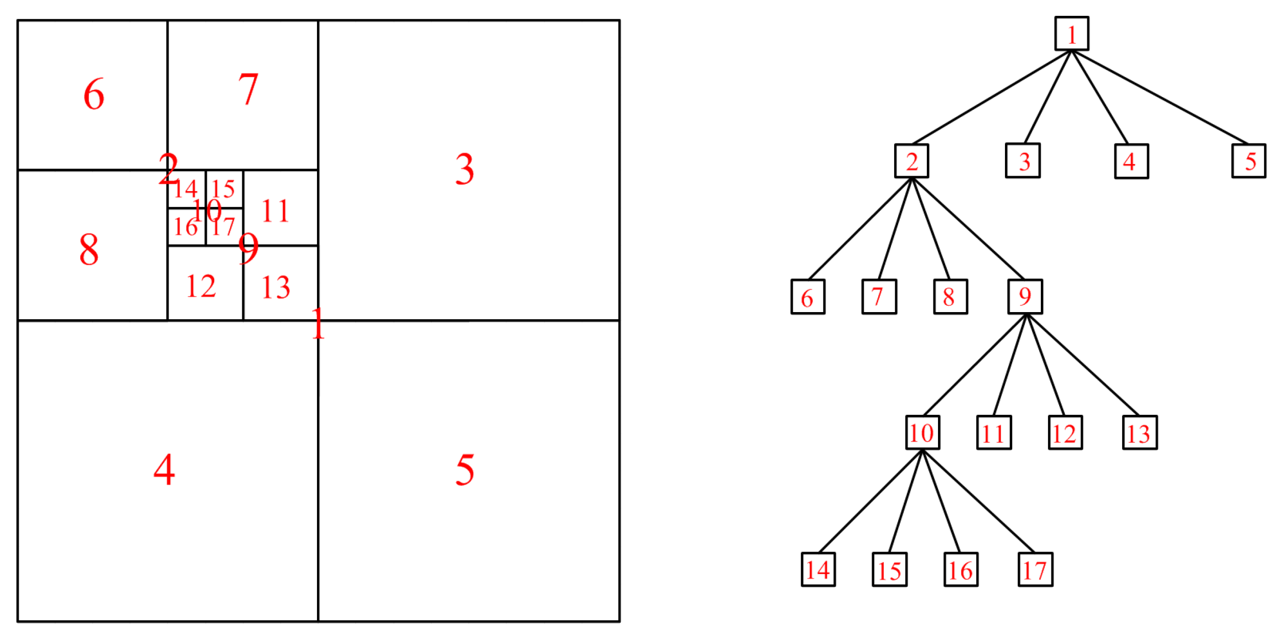
2.1. Mesh and Data Storage

The example of a cell-based mesh is shown in Figure 2. The mesh is based on a quadtree data structure: each child cell owns a parent cell, and each parent cell possesses four child cells. The mesh structure is managed and stored in a matrix table, as shown in

Table 1. Matrix table of mesh storage.

Table Index	Cell Number	Cell Type	NW Child Cell	NE Child Cell	SW Child Cell	SE Child Cell	Parent Cell Number	Level	Other Parameters
1	1	0	2	3	4	5	0	1	xy coordinate; refinement flag; coarse flag, and so on.
2	2	NW 1	6	7	8	9	1	2
3	3	NE	0	0	0	0	1	2
4	4	SW	0	0	0	0	1	2
…
10	10	NW	14	15	16	17	9	4
…
17	17	SE	0	0	0	0	10	5

¹ NW, NE, SW, SE: northwest, northeast, southwest, southeast.

. With the matrix table, the operations on refining a leaf cell into four new leaf cells and coarsening four leaf cells back into their parent cell are easily implemented. The leaf cells mean the child cells without descendants and are the cells that actually participated in numerical calculation. Additionally, query operations can be applied within the matrix table to trace the ancestors and descendants for any cell according to need. More detailed quadtree data structure can be seen in [33]. The Mesh refining () and Mesh coarsening () algorithms are shown in Algorithms 1 and 2, respectively

Algorithm 1 Mesh refining ()

for each cell  if a cell is a leaf cell and the refinement flag is 1   add four lines at the end of the matrix table;   fill mesh relation information (cell number, type, parent, level, xy coordinate, and so on);   interpolate initial flow variable using scatteredInterpolant() function (MATLAB function);  end end

Algorithm 2 Mesh coarsening ()

for each cell  if four leaf cells belong to a common parent cell and all coarse flags are 1   remove the lines of the four leaf cells;   modify the parent cell into leaf cell;   interpolate initial flow variable using the average mean of the four child cells;  end end

2.2. Neighbor Finding

In a numerical solution of PDE, the calculation on partial derivatives needs to use the information of neighbor cells. It is necessary to find all the neighbor cell numbers for a specified cell. The essential way to find the neighbors is to perform a mirror query operation, as shown in Figure 3. The algorithm can be divided into two steps: find neighbor of same size and find neighbor of smaller size. A more detailed explanation is illustrated in [34,35]. The Neighbor finding () algorithm is shown in Algorithm 3.

Algorithm 3 Neighbor finding ()

find neighbor of same size using ADJ function [34] according to a given direction;  store query path simultaneously;  find neighbor smaller size according to mirror query path using REFLECT function [34];

2.3. Neighbor Fixing

AMR procedure usually requires the mesh satisfying 2:1 condition between neighbors, meaning the number of neighboring cells to a specified cell is not allowed to exceed three. In other words, the level difference between adjacent cells should be limited to 0, 1, and −1. The 2:1 condition should be checked by the Neighbor finding () algorithm after mesh refinement and coarse operations. If the condition is not satisfied, the cells with more than three neighbor cells are divided into four cells by Mesh refining () algorithm operation.

The 2:1 condition in the diagonal direction is also mandatory in the present AMR procedure. If the condition is not implemented, the interpolation scheme on hanging nodes becomes much complex, which is not what we want. Figure 4 shows the mesh satisfying 2:1 condition after the Neighbor fixing () algorithm operation. The mesh was fixed from the mesh of Figure 2. The 24 cells indicated by red lines are newly added. The Neighbor fixing () algorithm is shown in Algorithm 4.

Algorithm 4 Neighbor fixing ()

while 1   if 2:1 condition is satisfied (checked by Neighbor finding () algorithm)    break;   end   for each direction (N S W E)    if the number of neighboring cells exceed three     set refinement flag to 1;    end   end   for each diagonal (NW NE SW SE)   if the absolute mesh level difference between central cell and diagonal cell exceeds 1     set refinement flag to 1;    end   end   perform Mesh refining () algorithm;  end

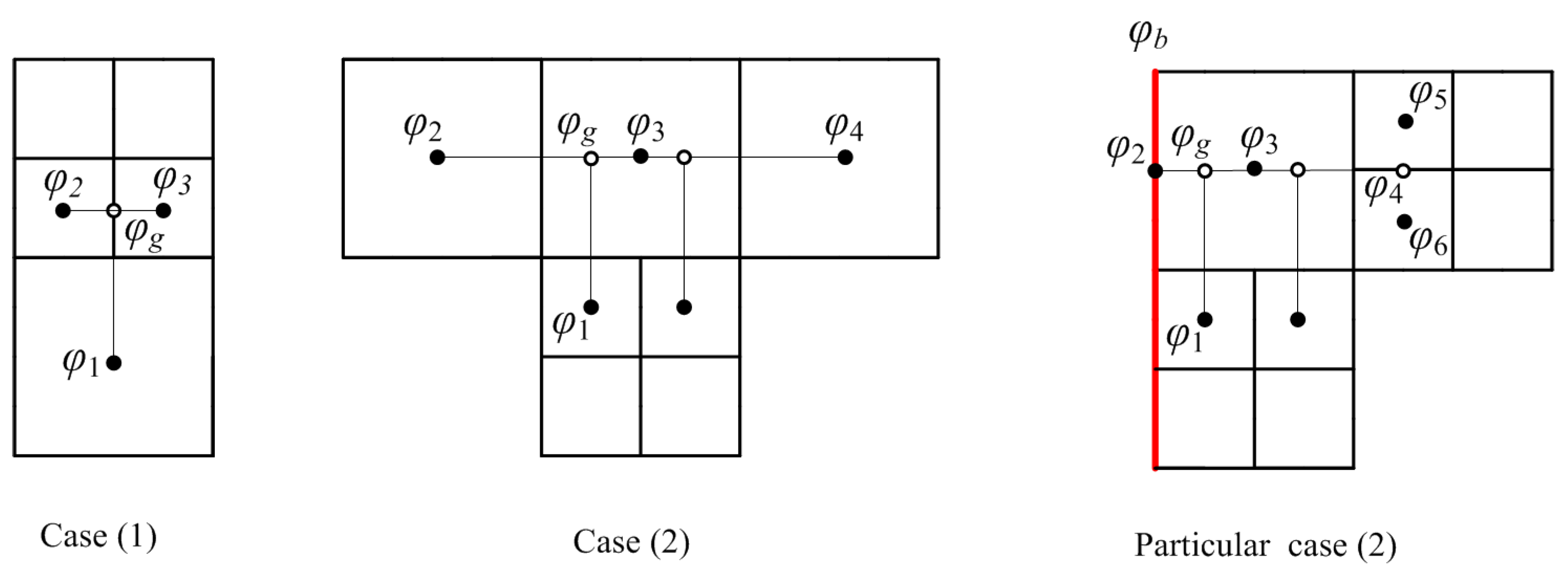
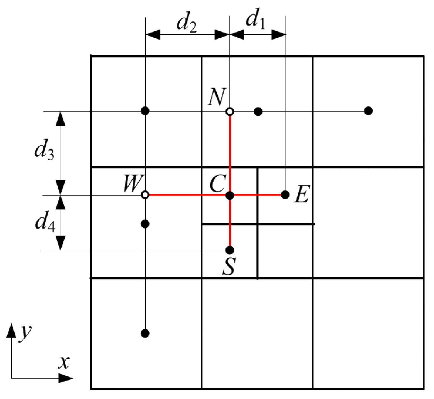
2.4. Handingnode Interpolating

Hanging nodes are created at the interfaces between different level cells (see in Figure 2) [36]. Two cases need to be considered: (1) the calculation upon the coarse grids needs the interpolation of fine grids and (2) the calculation upon the fine grids needs the interpolation of coarse grids, as shown in Figure 5. In the case of (1), the value of the ghost node is simply calculated by the average value as

$${\phi }_g=({\phi }_2+{\phi }_3)/2,$$

(1)

where φ is the flow variable. In the case of (2), the value of the ghost node is calculated by quadratic interpolation as

$${\phi }_g=a{x}_i{}^2+b{x}_i+c,$$

(2)

where a, b, c are the coefficients determined by φ₂, φ₃, φ₄, and x_i is the x coordinate of φ₁. The quadratic interpolation is implemented by MATLAB function [37]. If a boundary or fine grid is encountered, case (2) is considered a particular case. The values of φ₂ and φ₄ are, respectively, taken as the value of the boundary condition and the average value of the fine grid, as follows

$$\begin{array}{l}{\phi }_2={\phi }_b\\ {\phi }_4=({\phi }_5+{\phi }_6)/2\end{array}$$

(3)

where φ_b is the value of the boundary condition. The present interpolation hybridizes linear and quadratic rules. Although all quadratic interpolations are feasible, more effort in programming is required. Other methods such as prolongation and restriction methods to handle interpolation can be seen in [38]. The Handingnode interpolating () algorithm is shown in Algorithm 5.

Algorithm 5 Handingnode interpolating ()

if the neighbor cell is a boundary (Neighbor finding () algorithm returns zero)   return the value of boundary condition; else   if the number of neighbor cells is two (case (1))    return the average value using Equation (1);   end   if the number of neighbor cells is one and the level of neighbor cells is small than the level of the central cell (case (2))    return the quadratic interpolation value using Equation (2);   end   if the neighbor cell is the particular case (2)    return the quadratic interpolation value using Equation (3);   end  end

2.5. Periodic Matching

The west boundary and east boundary of the computational domain are paired into a periodic boundary condition. A periodic boundary condition is defined for the two boundaries where their values are linked in some defined way, such as interpolation or matching method. A matching method is applied to realize the periodic boundary condition. There are two steps to achieve the aim: (1) store the cell numbers of the west boundary and east boundary, respectively, and (2) conduct a pair matching operation according to the size of a cell.

The matching method is illustrated in Figure 6 and

Table 2. Periodic pair number table.

Cell Number of the West Boundary	Pair Number	Cell Number of the East Boundary	Pair Number
22	1	24	1
28	2	86	2
95	2	15	3
97	2
120	3
142	3

. In the first step, the cells of the west boundary and east boundary are detected by the Neighbor finding () algorithm according to the returned number of neighbor cells be zero or not. Owing to the Z-order filling curve (see below), the cell number is naturally in descending order along the y coordinate. Otherwise, a sort of operation needs to be performed by comparing y coordinate. Secondly, a pair number is added at each cell starting from the first two cells. The pair number is self-added when the size of the west boundary cell is equal to the size of the east boundary cell. For example, the cell of 28,95,97 matches the cell of 86 with the pair number of 2. Moreover, due to the number of neighbor cells of 86 exceeding three, dissatisfying the 2:1 condition, a mesh refinement operation should be conducted to the cell of 86 in the next step. The Periodic matching () algorithm is shown in Algorithm 6.

Algorithm 6 Periodic matching ()

detect the cells of west boundary and east boundary by Neighbor finding () algorithm;  create periodic pair number table simultaneously;  match the pair number according to the size of a cell;  if 2:1 condition is not satisfying (checked by Neighbor finding () algorithm)   preform Neighbor fixing () algorithm;  end

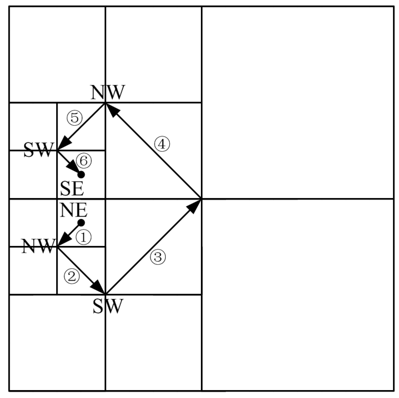
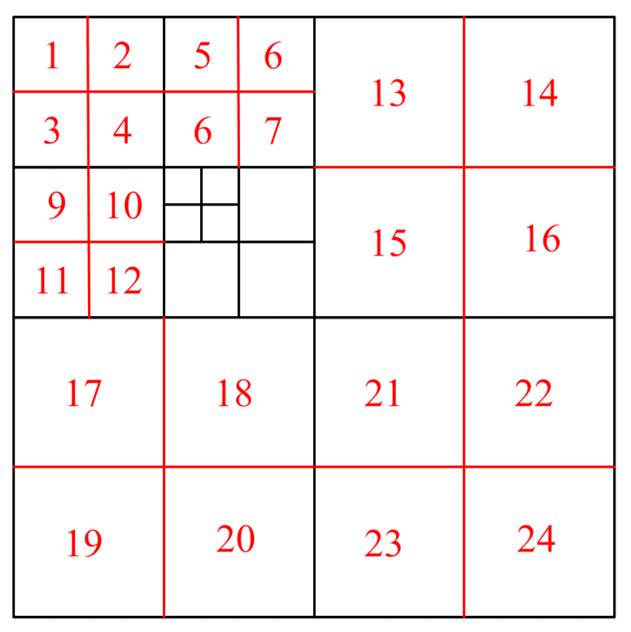
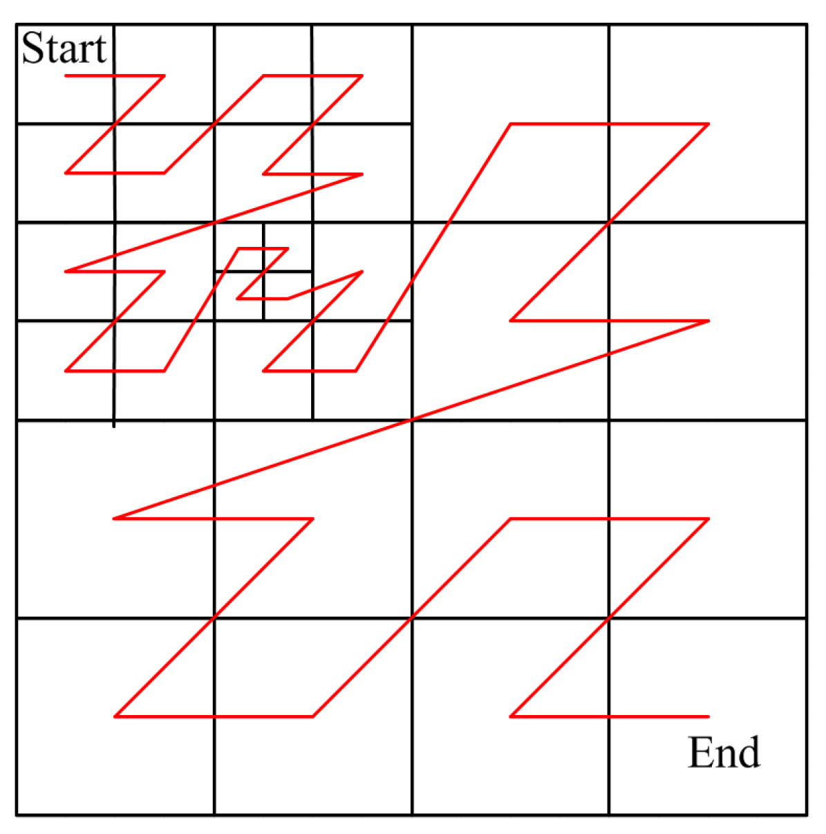
2.6. Z-Order Filling Curve

Z-order filling curve [39] is used to manage the solution order of the nonuniform mesh. A vector storing the ordered cell numbers is generated by the Z-ordering () algorithm, where the sequence of the cell numbers obeys the rule of the Z-order filling curve, as shown in Figure 7. The basic idea of the Z-ordering () algorithm is to travel the quadtree transversely under the sequence of NW→NE→SW→SE layer by layer. The Z-ordering () algorithm is shown in Algorithm 7.

Algorithm 7 Z-ordering ()

travel to the bottom NE cells as a start point;  store the travel path layer by layer simultaneously;  while the number of tagged cells is not equal to the total number of leaf cells   travel the leaf cells on the same layer under the sequence of NW→NE→SW→SE;   store the travel path layer by layer simultaneously;   go back to ancestor cell once the SE leaf cell is reached;  end

3. Difference Schemes on Nonuniform Mesh

The universal Reynolds equation [18] governing both liquid and cavitation regions is expressed as

$$\frac{\partial }{\partial x}\left(h^3\frac{\partial p}{\partial x}\right)+\frac{\partial }{\partial y}\left(h^3\frac{\partial p}{\partial y}\right)=6\mu U\frac{\partial (h\theta )}{\partial x},$$

(4)

where h is the film thickness, p is the liquid pressure, μ is the dynamic viscosity, U is the sliding speed, and θ is the density ratio. As mentioned above, AMR allows different numerical resolutions to exist in the computational domain; therefore, the regions have different sizes. As a result, the difference scheme for nonuniform mesh is different from that for uniform mesh. Figure 8 shows the parameter definition for the nonuniform difference scheme.

The difference scheme of the pressure flow term is derived as

$$\begin{array}{l}\frac{\partial }{\partial x}\left(h^3\frac{\partial p}{\partial x}\right)=\frac{p_E(h_C^3+h_E^3)}{d_1(d_1+d_2)}-\frac{p_C\left[d_2(h_C^3+h_E^3)+d_1(h_C^3+h_W^3)\right]}{d_1{d}_2(d_1+d_2)}+\frac{p_W(h_C^3+h_W^3)}{d_2(d_1+d_2)}\\ \frac{\partial }{\partial y}\left(h^3\frac{\partial p}{\partial y}\right)=\frac{p_N(h_C^3+h_N^3)}{d_3(d_3+d_4)}-\frac{p_C\left[d_4(h_C^3+h_N^3)+d_3(h_C^3+h_S^3)\right]}{d_3{d}_4(d_3+d_4)}+\frac{p_S(h_C^3+h_S^3)}{d_4(d_3+d_4)}\end{array}$$

(5)

The difference scheme of the shear flow term is derived as

$$6\mu U\frac{\partial (h\theta )}{\partial x}=6\mu U\frac{h_C{\theta }_C-h_W{\theta }_W}{d_2}.$$

(6)

Then, the explicit iterative schemes of p and θ can be written in the forms:

$$\begin{array}{l}{p}_{i,j}^{k+1}=\frac{A{p}_{i-1,j}^{k+1}+B{p}_{i+1,j}^k+C{p}_{i,j-1}^{k+1}+D{p}_{i,j+1}^k-F}{E}\\ {\theta }_{i,j}^{k+1}=\frac{A^{\prime }{\theta }_{i-1,j}^{k+1}{}_{}+B^{\prime }{\theta }_{i+1,j}^k+C^{\prime }{\theta }_{i,j-1}^{k+1}+D^{\prime }{\theta }_{i,j+1}^k-F^{\prime }}{E^{\prime }}\end{array}$$

(7)

where k is the number of iterations. The successive over-relaxation (SOR) method is applied to accelerate convergence. The SOR factors for p and θ are both taken as 1.2. The detailed solution strategy for Ausas’ algorithm can be seen in [18,19].

4. Error Estimation

Discretization error is defined as the difference between the exact solution of the discrete equation and the exact solution of the PDE. It is the primary source of numerical errors compared with round-off error and iterative error [40]. The Richardson extrapolation method is a recovery method and can be used to estimate discretization error [41].

The Richardson extrapolation method can obtain a more accurate solution than the available solution of the finest mesh. Assuming two numerical solutions have been calculated [42]: a fine grid with grid size h₁ and computed solution fc₁; and a coarse grid with grid size h₂ and computed solution fc₂, the extrapolated solution is evaluated as

$$f_{extr}=f_{c1}+\frac{f_{c1}-f_{c2}}{r^p-1},$$

(8)

where r is the grid refinement ratio r = h₂/h₁ and p is the order of accuracy. In other words, the more accurate solution is obtained by fine grid solution f_c1 and coarse grid solution f_c2 with weight coefficients of r^p/(r^p − 1) and -1/(r^p − 1). The discretization error for the fine grid solution f_c1 could be estimated as follows

$$err=f_{c1}-f_{extr}=\frac{f_{c2}-f_{c1}}{r^p-1}.$$

(9)

In the AMR method, the present existing mesh is treated as the fine mesh. The coarse mesh is generated by coarsening the whole mesh: all leaf cells are replaced by their parent cells. The value of r is therefore ensured to be constant 2. The order of accuracy p is also treated as constant. Thus, the denominator of Equation (9) is unchanged. The error estimation is taken as

$$err\propto \left|f_{c2}-f_{c1}\right|.$$

(10)

Equation (10) indicates that the difference between the solutions obtained on the two meshes at each point is proportional to the local discretization error at that point [27].

When the error estimation operation is finished, the next step is to decide the value of the unacceptably large error. A practical way is to sort these errors from large to small, and to refine the top cells with large errors. The number of the cells need to be refined is determined according to need. The mesh refinement operation can be repeated until the solution is satisfactory.

5. Results and Discussion

The implementation steps of the AMR method are to (1) obtain a preliminary solution on initial coarse mesh, (2) obtain a more accurate solution by a refined mesh operation, and (3) repeat step (2) until a sufficiently accurate solution satisfying the need. The refinement strategy has a significant effect on the final mesh. It affects not only the accuracy of the solution but also the computational cost. An appropriate refinement strategy can realize a more efficient solution.

Although the use of variable gradient as a refinement indicator is more natural, the paper adopted a posteriori error estimation to refine the areas where the discretization error was large. As mentioned above, the Richardson extrapolation method is a simple way to find the area where it needs to be refined.

Pressure and density ratio are the main flow variables of a bearing film. If an individual parameter (pressure or density ratio) is used as error estimation, this is inappropriate in Ausas’ cavitation algorithm since the pressure is always constant cavitation pressure in the cavitation region, and the density ratio is always constant 1 in the liquid region. The refinement on the whole bearing film is impossible. Significant discretization error always exists in the cavitation region or liquid region. Thus, pressure and density ratio are both taken as the variables to estimate error. Two cases were studied below to show the AMR results.

The first case is the cavitated journal bearing studied by Cupillard et al. [8,9] and Brewe [10]. The bearing is a finite type, with L/D = 4/3 (D = 100 mm), operating in the condition of ε = 0.60, n = 459 r/min, p_c = 28 kPa (a), and μ = 0.0127 Pa·s. The solution of the three-time refined mesh is compared with the solution of the corresponding uniform mesh and the experimental data. The initial mesh is taken as a very coarse mesh with 16 × 16 cells. This mesh is generated by recursively refining the whole mesh four times. In the first refinement, 30 cells in the liquid region and 40 cells in the cavitation region were tagged to be refined. The tagged cells were the cells of the coarsen mesh with 8 × 8 cells in the implementation of the Richardson extrapolation method. After the refinement operation, the number of the cells refined was 240. It was lower than the expected number of grids, 280, as calculated by 70 × 4. This is because some of the tagged cells with large errors were common in the cavitation and liquid regions. In the subsequent refinements, 90 and 300 cells in the liquid region and 40 and 180 cells in the cavitation region were tagged to be refined for the second and third refinements, respectively. It is noted that the number of cells tagged was empirically determined according to the initial numerical tests. Although the refinement strategy is empirical, it still shows the law that the ratio of the tagged number to the total number reduces with the increase in total cell numbers. As shown in

Table 3. Refinement strategy for the two cases.

Bearings	Refinement Level	Number of Tagged Cells for Pressure	Number of Tagged Cells for Density Ratio	Number of Cells Actually Refined (A)	Total Number of Cells before Refinement (B)	Refinement Ratio (A/B)
Case 1: journal bearing	1	30	40	240	265	91%
	2	90	40	672	1024	65%
	3	300	180	1664	4096	41%
Case 2: thrust bearing	1	30	40	252	265	95%
	2	150	60	776	1024	76%
	3	350	180	1960	4096	48%

, the refinement ratios are 91%, 65%, and 41% in descending order. The refinement strategy indicates that the discretization error of the coarse mesh should be reduced sufficiently. This is because the coarse mesh has the largest discretization error, where the discretization error is proportional to the power p of the grid spacing h.

Figure 9 shows the pressure and density ratio for the final refined mesh. It can be seen that the refined meshes tagged by the pressure-based error estimation were basically distributed in the region with large pressure gradients, and the refined meshes tagged by density ratio-based error estimation were basically distributed in the region of cavitation interfaces where the density ratio gradients were also large. This behavior indicated that the discretization error was concentrated in the area with large variable gradients. Figure 10 compares the pressure distribution for the AMR results, uniform mesh results, and experimental results provided by Jakobsson and Floberg [12] and Olsson [13]. The pressure obtained by the AMR method is nearly consistent with that obtained by the uniform mesh (128 × 128 cells), and there is a slight difference in the experimental results. The number of the final refined mesh is 7984, while the number of the uniform mesh is 16,384. The AMR method provides almost the same accuracy results while the number of cells is reduced to around 50% of the uniform mesh. The computational efficiency is shown to be effectively improved.

The second case is the dimple-enhanced seal-like thrust bearing investigated by Qiu and Khonsari [22]. The bearing surface was textured with duplicated micro circular holes. The variation of the hole height results in a divergence and convergence clearance region. Hence, oil film rupture and reformation simultaneously occur around the hole. The bearing was operated in the condition of r₀= 750 μm, h_g = 10 μm, L = 3 mm, h₀ = 4 μm, μ = 0.0035 Pa·s, U = 1.45 m/s, p_c = 0.9 × 10⁵ Pa (a), p_a = 1.0 × 10⁵ Pa (a). The refinement strategy for the bearing is listed in Table 3. The refinement ratios were 91%, 76%, and 48% for the three-time refinements. They are higher than those of case 1. A more computational cost was indicated to be paid. The solution of the three-times refined mesh is compared with the solution of the corresponding uniform mesh and the solution provided by Qiu and Khonsari [22], as shown in Figure 11 and Figure 12. It can be seen that the AMR solution is close to the solution of the uniform mesh (128 × 128 cells) with a small difference compared with the solution provided by Qiu and Khonsari [22]. The difference is mainly reflected by the value of maximum pressure. Ausas’ algorithm is sensitive to the number of grids. Insufficient number of grids often leads to high maximum pressure. The difference is acceptable under the current refinement strategy. The number of the final refined mesh is 9220, which is 56% of the uniform mesh. The AMR method provides almost the same accuracy solution while the computational cost is saved.

6. Conclusions

A quadtree-based AMR procedure was developed for bearing cavitation simulation. The universal Reynolds equation was numerically solved on the nonuniform mesh by Ausas’ cavitation algorithm. The pressure and density ratio were both taken as the indicators of the error estimation with the Richardson extrapolation method. The investigated cases showed that the AMR method provided nearly the same accuracy results compared with the uniform mesh, while the number of mesh was reduced to 50–60% of the number of the uniform mesh. The computational efficiency was effectively improved. The AMR method is suggested to be a potential tool for bearing cavitation simulation.

References

1. Mishra, P.C.; Rahnejat, H. 20-Tribology of big-end bearings. In Tribology and Dynamics of Engine and Powertrain; Rahnejat, H., Ed.; Woodhead Publishing: Sawston, UK, 2010; pp. 635–659. [Google Scholar]
2. Manser, B.; Belaidi, I.; Hamrani, A.; Khelladi, S.; Bakir, F. Performance of hydrodynamic journal bearing under the combined influence of textured surface and journal misalignment: A numerical survey. C. R. Méc. 2019, 347, 141–165. [Google Scholar] [CrossRef]
3. Tauviqirrahman, M.; Afif, M.F.; Paryanto, P.; Jamari, J.; Caesarendra, W. Investigation of the Tribological Performance of Heterogeneous Slip/No-Slip Journal Bearing Considering Thermo-Hydrodynamic Effects. Fluids 2021, 6, 48. [Google Scholar] [CrossRef]
4. Miwa, R.; Miyanaga, N.; Tomioka, J. Appearance of Hysteresis Phenomena on Hydrodynamic Lubrication in a Seal-Type Thrust Bearing with Dimples. Materials 2021, 14, 5222. [Google Scholar] [CrossRef] [PubMed]
5. Dowson, D.; Taylor, C.M. Cavitation in Bearings. Annu. Rev. Fluid Mech. 1979, 11, 35–65. [Google Scholar] [CrossRef]
6. Sun, D.; Li, S.; Fei, C.; Ai, Y.; Liem, R.P. Investigation of the effect of cavitation and journal whirl on static and dynamic characteristics of journal bearing. J. Mech. Sci. Technol. 2019, 33, 77–86. [Google Scholar] [CrossRef]
7. Shen, C.; Khonsari, M.M. On the Magnitude of Cavitation Pressure of Steady-State Lubrication. Tribol. Lett. 2013, 51, 153–160. [Google Scholar] [CrossRef]
8. Cupillard, S.; Cervantes, M.; Glavatskih, S. A CFD study of a finite textured journal bearing. In Proceedings of the IAHR Symposium on Hydraulic Machinery and Systems, Foz do Iguaçu, Brazil, 27–31 October 2008. [Google Scholar]
9. Cupillard, S.; Glavatskih, S.; Cervantes, M.J. Computational Fluid Dynamics Analysis of a Journal Bearing with Surface Texturing. Proc. Inst. Mech. Eng. Part. J. J. Eng. Tribol. 2008, 222, 97–107. [Google Scholar] [CrossRef]
10. Brewe, D.E. Theoretical Modeling of the Vapor Cavitation in Dynamically Loaded Journal Bearings. J. Tribol. 1986, 108, 628–637. [Google Scholar] [CrossRef] [Green Version]
11. Elrod, H.G. A Cavitation Algorithm. J. Lubr. Technol. 1981, 103, 350–354. [Google Scholar] [CrossRef]
12. Jakobsson, B.; Floberg, L. The Finite Journal Bearing, Considering Vaporization. Trans. Chalmers Univ. Technol. 1957, 190. Available online: https://www.worldcat.org/title/finite-journal-bearing-considering-vaporization/oclc/718857301 (accessed on 5 August 2021).
13. Olsson, K. Cavitation in Dynamically Loaded Bearings. Trans. Chalmers Univ. Technol. 1965, 308, 155–162. [Google Scholar]
14. Gropper, D.; Wang, L.; Harvey, T.J. Hydrodynamic Lubrication of Textured Surfaces: A Review of Modeling Techniques and Key Findings. Tribol. Int. 2016, 94, 509–529. [Google Scholar] [CrossRef] [Green Version]
15. Braun, M.J.; Hannon, W.M. Cavitation formation and modelling for fluid film bearings: A review. Proc. Inst. Mech. Eng. Part. J. J. Eng. Tribol. 2010, 224, 839–863. [Google Scholar] [CrossRef]
16. Fesanghary, M.; Khonsari, M.M. A Modification of the Switch Function in the Elrod Cavitation Algorithm. J. Tribol. 2011, 133, 024501. [Google Scholar] [CrossRef]
17. Nitzschke, S.; Woschke, E.; Schmicker, D.; Strackeljan, J. Regularised cavitation algorithm for use in transient rotordynamic analysis. Int. J. Mech. Sci. 2016, 113, 175–183. [Google Scholar] [CrossRef]
18. Ausas, R.; Ragot, P.; Leiva, J.; Jai, M.; Bayada, G.; Buscaglia, G.C. The Impact of the Cavitation Model in the Analysis of Microtextured Lubricated Journal Bearings. J. Tribol. 2007, 129, 868–875. [Google Scholar] [CrossRef]
19. Ausas, R.F.; Jai, M.; Buscaglia, G.C. A Mass-Conserving Algorithm for Dynamical Lubrication Problems With Cavitation. J. Tribol. 2009, 131, 031702. [Google Scholar] [CrossRef]
20. Giacopini, M.; Fowell, M.T.; Dini, D.; Strozzi, A. A Mass-Conserving Complementarity Formulation to Study Lubricant Films in the Presence of Cavitation. J. Tribol. 2010, 132, 041702. [Google Scholar] [CrossRef]
21. Woloszynski, T.; Podsiadlo, P.; Stachowiak, G.W. Efficient Solution to the Cavitation Problem in Hydrodynamic Lubrication. Tribol. Lett. 2015, 58, 18. [Google Scholar] [CrossRef]
22. Qiu, Y.; Khonsari, M.M. On the Prediction of Cavitation in Dimples Using a Mass-Conservative Algorithm. ASME J. Tribol. 2009, 131, 041702. [Google Scholar] [CrossRef]
23. Miraskari, M.; Hemmati, F.; Jalali, A.; Alqaradawi, M.Y.; Gadala, M.S. A Robust Modification to the Universal Cavitation Algorithm in Journal Bearings. J. Tribol. 2016, 139, 031703. [Google Scholar] [CrossRef]
24. Berger, M.J.; Oliger, J. Adaptive mesh refinement for hyperbolic partial differential equations. J. Comput. Phys. 1984, 53, 484–512. [Google Scholar] [CrossRef]
25. Stadler, G.; Gurnis, M.; Burstedde, C.; Wilcox, L.C.; Alisic, L.; Ghattas, O. The Dynamics of Plate Tectonics and Mantle Flow: From Local to Global Scales. Science 2010, 329, 1033–1038. [Google Scholar] [CrossRef] [PubMed]
26. Liu, S.; King, S.D. A benchmark study of incompressible Stokes flow in a 3-D spherical shell using ASPECT. Geophys. J. Int. 2019, 217, 650–667. [Google Scholar] [CrossRef]
27. Berger, M.J.; Colella, P. Local adaptive mesh refinement for shock hydrodynamics. J. Comput. Phys. 1989, 82, 64–84. [Google Scholar] [CrossRef] [Green Version]
28. Waltz, J.; Bakosi, J. A coupled ALE–AMR method for shock hydrodynamics. Comput. Fluids 2018, 167, 359–371. [Google Scholar] [CrossRef]
29. Mirzadeh, M.; Guittet, A.; Burstedde, C.; Gibou, F. Parallel level-set methods on adaptive tree-based grids. J. Comput. Phys. 2016, 322, 345–364. [Google Scholar] [CrossRef] [Green Version]
30. Zhang, C.; Fakhari, A.; Li, J.; Luo, L.-S.; Qian, T. A comparative study of interface-conforming ALE-FE scheme and diffuse interface AMR-LB scheme for interfacial dynamics. J. Comput. Phys. 2019, 395, 602–619. [Google Scholar] [CrossRef]
31. Dai, W.W. Issues in adaptive mesh refinement. In Proceedings of the 2010 IEEE International Symposium on Parallel & Distributed Processing, Workshops and Phd Forum (IPDPSW), Atlanta, GA, USA, 19–23 April 2010; pp. 1–8. [Google Scholar]
32. Burstedde, C.; Wilcox, L.C.; Ghattas, O. p4est: Scalable algorithms for parallel adaptive mesh refinement on forests of octrees. SIAM J. Sci. Comput. 2011, 33, 1103–1133. [Google Scholar] [CrossRef] [Green Version]
33. Angelo, A. A Brief Introduction to Quadtrees and Their Applications. In Proceedings of the Style file from the 28th Canadian Conference on Computational Geometry, Vancouver, BC, Canada, 3–5 August 2016. [Google Scholar]
34. Samet, H. Neighbor finding techniques for images represented by quadtrees. Comput. Graph. Image Process. 1982, 18, 37–57. [Google Scholar] [CrossRef]
35. David. Advanced Octrees 4: Finding neighbor nodes. Available online: https://geidav.wordpress.com/2017/12/02/advanced-octrees-4-finding-neighbor-nodes/ (accessed on 20 March 2021).
36. Martin, D.F. Solving Poisson’s Equation Using Adaptive Mesh Refinement; Citeseer: University Park, PA, USA, 1996. [Google Scholar]
37. Omran, S. Quadratic Equation Interpolation, MATLAB Central File Exchange. Retrieved. 2021. Available online: https://www.mathworks.com/matlabcentral/fileexchange/41298-quadratic-equation-interpolation (accessed on 14 April 2021).
38. Popinet, S. A quadtree-adaptive multigrid solver for the Serre–Green–Naghdi equations. J. Comput. Phys. 2015, 302, 336–358. [Google Scholar] [CrossRef] [Green Version]
39. Kilimci, P.; Kalipsiz, O. Indexing of spatiotemporal Data: A comparison between sweep and z-order space filling curves. In Proceedings of the International Conference on Information Society (i-Society 2011), London, UK, 27–29 June 2011; pp. 450–456. [Google Scholar]
40. Phillips, T.S.; Roy, C.J. A New Extrapolation-Based Uncertainty Estimator for Computational Fluid Dynamics. J. Verif. Valid. Uncertain. Quantif. 2017, 1, 041006. [Google Scholar] [CrossRef]
41. Phillips, T. Extrapolation-Based Discretization Error and Uncertainty Estimation in Computational Fluid Dynamics. Master’s Thesis, Virginia Polytechnic Institute and State University, Blacksburg, VA, USA, 2012. [Google Scholar]
42. Wahba, E.M. Non-systematic grid refinement procedures for computational fluid dynamics. Appl. Math. Comput. 2013, 225, 829–842. [Google Scholar] [CrossRef]
Figure 1. Different types of adaptive mesh refinement: (a) block-based AMR method; (b) cell-based AMR method.
Applsci 11 09879 g001
Figure 2. General quadtree mesh structure.
Applsci 11 09879 g002
Figure 3. Neighbor finding () algorithm.
Applsci 11 09879 g003
Figure 4. The mesh satisfying 2:1 condition.
Applsci 11 09879 g004
Figure 5. Two kinds of cases for hanging nodes (blank circle indicates ghost nodes).
Applsci 11 09879 g005
Figure 6. An example of periodic boundary condition.
Applsci 11 09879 g006
Figure 7. Z-order filling curve.
Applsci 11 09879 g007
Figure 8. Parameter definition for the nonuniform difference scheme.
Applsci 11 09879 g008
Figure 9. Final refined mesh for journal bearing: (a) pressure distribution; (b) density ratio distribution.
Applsci 11 09879 g009
Figure 10. Comparison of pressure distribution between different results for y = 50 mm.
Applsci 11 09879 g010
Figure 11. Final refined mesh for thrust bearing: (a) pressure distribution; (b) density ratio distribution.
Applsci 11 09879 g011
Figure 12. Comparison of pressure distribution between different results for y = 1.5 mm.
Applsci 11 09879 g012