Featured Application
The proposed control strategy can be used to impose the closed-loop system dynamics behaviour in flexible mechatronic systems in the presence of time delay, such as robots where delay is introduced by sensors, actuators or communication networks, or systems with inherent delay such as milling and cutting machines. The use of receptances remarkably simplifies the controller design.
Abstract
This paper proposes a method for active vibration control to a two-link flexible robot arm in the presence of time delay, by means of robust pole placement. The issue is of practical and theoretical interest as time delay in vibration control can cause instability if not properly taken into account in the controller design. The controller design is performed through the receptance method to exactly assign a pair of pole and to achieve a given stability margin for ensuring robustness to uncertainty. The desired stability margin is achieved by solving an optimization problem based on the Nyquist stability criterion. The method is applied on a laboratory testbed that mimic a typical flexible robotic system employed for pick-and-place applications. The linearization assumption about an equilibrium configuration leads to the identification of the local receptances, holding for infinitesimal displacements about it, and hence applying the proposed control design technique. Nonlinear terms, due to the finite displacements, uncertainty, disturbances, and the coarse encoder quantization, are effectively handled by embedding the robustness requirement into the design. The experimental results, and the consistence with the numerical expectations, demonstrate the method effectiveness and ease of application.
1. Introduction
The presence of time delay in controlled systems degrades the closed-loop performance if it is not taken into account in the controller design, and in the worst case, might lead to instability. For example, time delay is due to the physical and operational characteristics of the system, e.g., due to friction [1,2] or due to nature of some manufacturing processes as milling [3] or metal cutting [4]. Delays are also caused by the mechatronic instrumentation employed in experimental real-time systems. In this case, the primary sources of delays are sensors, actuators, and communication networks [5].
Over the years, the most eminent researchers tackled this problem through several control solutions, for example, integer and fractional order PID control [6], model predictive control [7], Smith predictor [5,8,9], communication disturbance observer [10,11], sliding mode control [12], and switching control [13].
A technique attracting an ever-growing interest for active vibration control of vibrating linear systems with time delay is pole placement, borrowed by the traditional approaches for systems without time delay [14,15]. The seminal receptance method for pole placement [16] has been extended in [17] accounting also for time delay. The extension to partial pole placement requires that a subset of the system poles is assigned while the remaining unassigned poles are kept unchanged with respect to the open-loop configuration. This problem has been tackled in [18]. The same problem has been solved using the system matrices instead of the measured receptances in [19] for the single input case and later extended for multi-input control in [20].
The papers previously quoted require evaluating a posteriori the stability of the closed-loop system. Recently, a two-stage method that embeds an a priori stability condition has been developed by Belotti and Richiedei in [21]. It relies on the powerful theory of Linear Matrix Inequalities (LMI) and ensures the placement of the dominant poles of interest while imposing stability of the remaining unassigned poles, either those due to the mechanical resonances and those induced by the time delay. This method uses both the measured receptances to assign the dominant poles, and the system matrices, that are required by the LMIs.
Inspired by the controller parametrization proposed in the paper of Belotti and Richiedei, a method that only exploits the measured receptances has been proposed by Araujo, Dantas, and Dorea in [22]. The state feedback control gains are computed to assign the dominant poles and simultaneously impose the closed-loop system stability and robustness through the generalized Nyquist criterion. Robustness is achieved using the sensitivity function of the loop gain as an index and the problem is solved through a genetic algorithm.
In this paper, such a method is experimentally applied to control a flexible robot arm that mimics a typical system for pick-and-place applications. The arm flexibility is due to the passive joint torsional spring, that is an approach commonly used to represent flexibility of robots through a lumped model (see, e.g., the milestone paper in [23]). Time delays in this kind of system usually arise due to the instrumentation employed for real-time control. The proposed method is implemented by means of local linearization of the nonlinear dynamic model of the flexible robot and nonlinearities, as well as other uncertainty sources, are handled by imposing adequate robustness in the controller design.
2. Definitions
Let us consider a N-DOF (degree of freedom) linear, time-invariant, vibrating system. Its mass, damping, and stiffness matrices are respectively denoted by and its equations of motion are therefore
where is the generalized displacement vector and , its derivatives with respect to the time t. is the force influence matrix and is the independent external control force.
The rank-one control law for a regulation problem in the case of state feedback control, and by assuming that delay affects the measurements, is defined as follows:
where are the velocity and displacement gain vectors and and the respective time delays. State references are omitted in Equation (2) since do not affect the eigenstructure; their inclusion is, however, trivial.
The closed-loop controlled system in the Laplace domain denoted by s is inferred from Equation (1), leading to
The left-hand side of Equation (3) is the transcendental characteristic equation of the closed-loop system, , whose i-th solution is the i-th closed-loop pole of the system. If then is a polynomial and therefore the system features eigenpairs that completely describe the system dynamics. Conversely, as studied in this paper, if the time delays are not null, the characteristic equation has an infinite number of roots: roots are the “primary roots”, while an infinite number of “secondary roots” (often denoted as the “latent roots”) arise [21,24].
3. Method Description
3.1. Placement of the Closed-Loop Poles
In this paper, the problem of robust pole placement in delayed systems with single-input control is tackled: given a set of desired closed-loop poles, the goal is to compute the control gain vectors and such that the poles are assigned at the prescribed locations and the controlled system satisfy a certain robustness condition. Additionally, it is assumed that the system matrices , and are not available and therefore the proposed method should just relies on the measured receptances. Indeed, the knowledge of the system receptances suffices to describe the system properties without the need of knowing the system matrices and therefore allows for designing the controller [16,22].
The open-loop receptance matrix of the system is defined as [16]
its generic -th entry is the transfer function from the force applied to the q-th coordinate to the displacement of the p-th coordinate.
The closed-loop receptance matrix is simply inferred from Equation (3), leading to
The closed-loop poles are characterized by those complex values of s that set to zero the denominator of Equation (6):
The problem of finding the control gains and that assign the desired closed-loop poles can be written as follows [17,22]:
where , with . The system can be formulated, with a more compact notation as the usual form of a linear system, , with obvious meaning of the notation from Equation (8).
In the case of the complete assignment of the closed-loop poles, i.e., , if the matrix on the left-hand side of Equation (8) is invertible, the solution of the linear system is: . Therefore, the solution to the complete pole placement problem is unique. Conversely, in the case of partial pole placement desired closed-loop poles are assigned. In this scenario the linear system in Equation (8) has infinite solutions .
In particular, if , the solution of is
where is the particular solution of the non-homogeneous equation. While, is the solution of the homogeneous equation . Finally, the solution of Equation (8) is more conveniently formulated as follows [21,26,27]:
where is a matrix whose columns span the null space of , i.e., , while is an arbitrary vector. Any choice of vector does not perturb the assigned poles. Therefore, can be wisely chosen to accomplish secondary tasks, such as assigning other poles, stabilizing the systems or obtaining the desired robustness. In the following section a strategy to compute ensuring the desired robustness will be discussed, by taking advantage of the receptance-based method proposed by Araujo, Dantas, and Dorea in [22].
3.2. Introduction of the Robustness Condition
Due to the strong influence of time delays, satisfaction of Equations (7) and (8), does not guarantee that the set of desired closed-loop poles are “primary roots”. The search for a solution with stability and performance/robustness certificate must be carried out with focus on Equation (10). Frequency domain techniques can successfully deal with rational and transcending transfer functions, including those resulting from time delay in linear systems [28,29]. In particular, the Nyquist stability criterion [30], a cornerstone of classical control theory, can be straightforwardly applied to the characteristic Equation (7), in conjunction with the robustness margins approach [29,31] by taking the loop-gain transfer function as
A search strategy based on the maximum peak of the sensitivity function () associated with this loop-gain can offer a trade-off between robustness and performance for the closed-loop controlled system [29]. As the system parameters are usually uncertain, robustness is a significant issue in the controller design [32]. The peak is related with a disk with center in the critical abscissa of instability and radius equal to . This disk establishes an acceptable distance from the Nyquist curve of from the point . The Nyquist criterion states that, for an open-loop system with all poles on the left half-plane, the closed-loop system will be stable if the Nyquist curve of does not encircle the point . The larger the disk radius, the more robust the system is with respect to perturbations on the nominal loop-gain . Then, the design problem can be formulated as that of computing the feedback gains of the parametrized family, in Equation (7), with a simultaneous guarantee that the Nyquist curve of the loop-gain lies in a safe distance of to the critical point. This problem can be approached through the following minimization formulation:
The second constraint in Equation (12) assures that every cross point on the real axis lies on the right of the disk, avoiding then encirclement of the critical point . Notice that the frequency must belong to a frequency range , suitable to a representative Nyquist plot. This range can be, as an instance, the same used in the experimental identification of the system receptance. Moreover, for underactuated systems, only the partial information must be known to compute the gains.
3.3. Numerical Implementation Details
The objective function and the stability constraint in Equation (12) are hard to approach with gradient-based methods. It is well known that genetic algorithm-based search (GA) can be more accurate to solve optimization problems of moderate complexity, as non-convex ones [33]. A GA implementation was developed, tailored to find a solution for Equation (12).
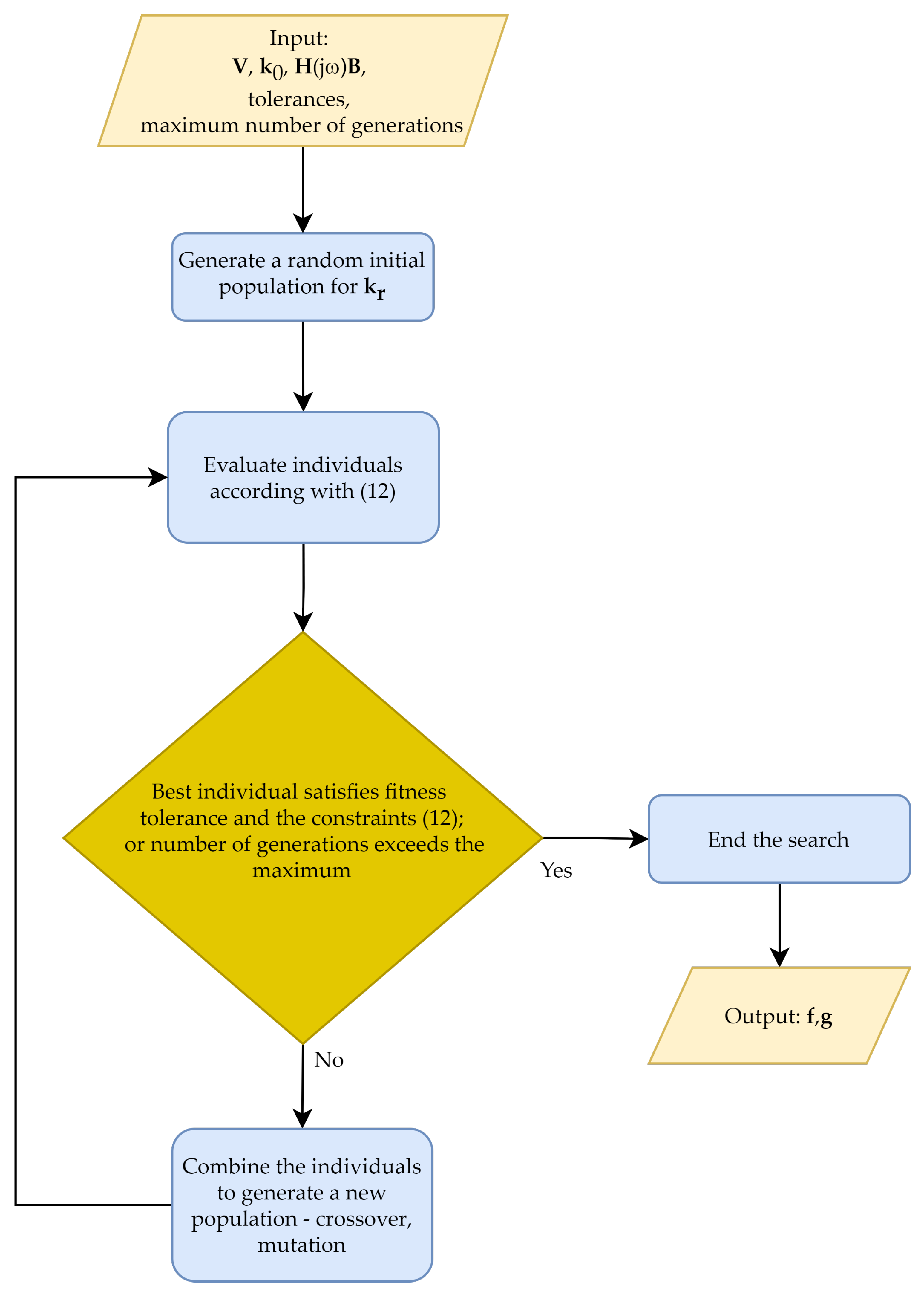
Given the particular solution and the null space basis , the solution for the optimization problem in Equation (12) is achieved by following some simple steps. First, randomly define a set of vectors. Then, evaluate each one individual in this set for fitness and constraints. The procedure is summarized in the flowchart displayed in Figure 1. In the step devoted to update the population, functions to execute crossover and mutation can be chosen and adjusted following the theory of Genetic Algorithms [34]. In the step of individuals combination, first, it is ensured that the best rated individual in the actual generation is saved for the next one. Furthermore, it is selected some possible solutions to gives rise to a new population. Those are called parents, and they are chosen in a draw where the best-rated individuals have a greater chance of being selected. Once the parents are chosen, the combination is done, and this could be achieved using any kind of crossover methods available in the GA theory. Finally, a percentage of individuals is slightly randomly modified in the mutation process. In the test cases of the following sections, GA was programmed for (i) a maximum number of generations of one-hundred and (ii) a fitness function tolerance of .

Figure 1.
The flowchart of the numerical procedure to feedback gains design.
4. Test Case: A Two-Link Flexible Robot Arm
4.1. System Description
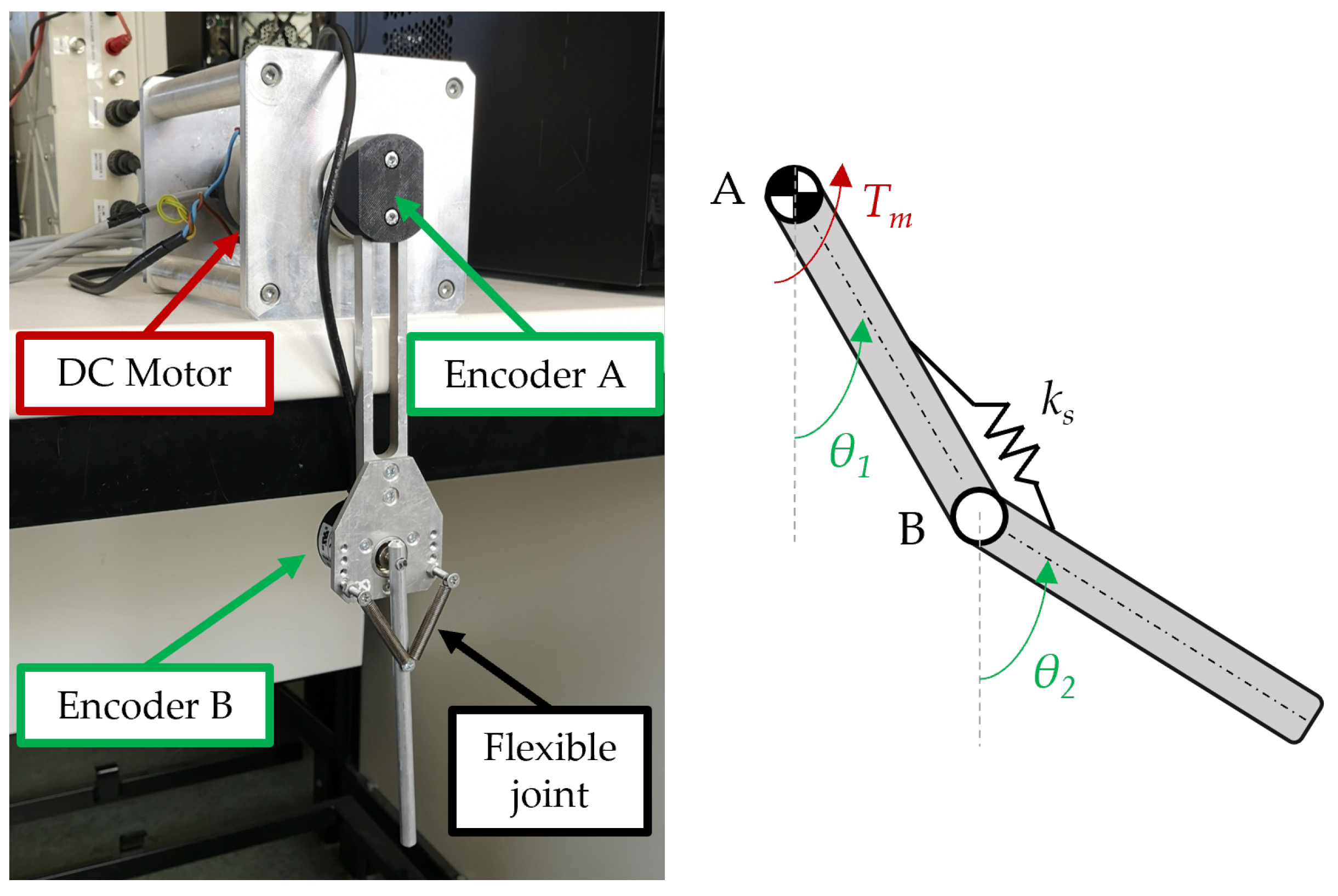
The proposed control strategy is applied to the two-link flexible robot arm shown in Figure 2, already employed in [35] as a benchmark for vibration control.

Figure 2.
The two-link flexible robot arm and its kinematic scheme.
The system has two DOFs, described by the absolute rotations and . The revolute joint A is actuated through the torque exerted by a DC motor. The revolute joint B is passive with a torsional spring (made through two linear springs). The flexibility of the robotic arm is mimicked by the linear torsional spring located at the passive joint, while the links are rigid. This yields to an underactuated two-link robot arm with and . All the relevant system parameters are defined in Table 1.

Table 1.
System parameters.
The link rotations are measured through two incremental encoders, with 500 pulses per revolute. This low resolution perturbs the sensed displacements and the estimated speeds, that are obtained through numerical derivatives, and therefore attention to the robustness issue should be paid in the controller design.
The DC motor driving joint A has the moment of inertia , to be summed to the moment of inertia of the coupling. The length of the first link, connected to joint A, is , its mass and the moment of inertia with respect to point A is . The length of the second link, connected to joint B, is , its mass and the moment of inertia with respect to point B is . The mass of the second encoder together with the mounting bracket mass should be accounted for as well, i.e., .
The nonlinear model of the system is obtained through the Lagrangian approach, leading to the following equation of motion (g is the gravitational acceleration):
In the presence of small displacements about an equilibrium configuration, the system in Equation (13) can be locally linearized to apply the theory of linear control. Therefore, local receptances can be experimentally identified to apply the theory proposed in this paper. To show the features of the linearized model, although it is not used by the receptance-based approach here proposed to controller design, the linearized model around the vertical equilibrium position, i.e., , is described by the following matrices [35]:
where is the damping matrix.
The deviations between the nonlinear model and the linearized one, and thus between the nonlinear model and the local receptances, that arise with finite link rotations about the equilibrium, should be considered as uncertainty sources that the controller should get rid through adequate robustness. Other perturbations affect the controller design: the aforementioned low resolution of the encoders, errors, and uncertainty in the receptance measurements, non-viscous friction terms, and some unpredictable dynamics that will be discussed in Section 4.2.1.
In all the tests, both numerical and experimental, it is assumed that s and s. These severe values are chosen by means of example to highlight some benefits of the proposed method. The delays have been introduced in the real-time control scheme, developed through Real Time Simulink (running with a sample time ms).
Two different assignment tasks are performed to highlight different features of the proposed method and then are experimentally applied to provide further evidences.
4.2. Numerical Assessment
4.2.1. Test Case 1: Increasing Damping of the Second Vibrational Mode
The state-feedback controller is designed such that the second pole pair is assigned to , i.e., damping is increased to while the damped natural frequency is kept unchanged. The maximum peak of the sensitivity function is imposed to to ensure adequate robustness.
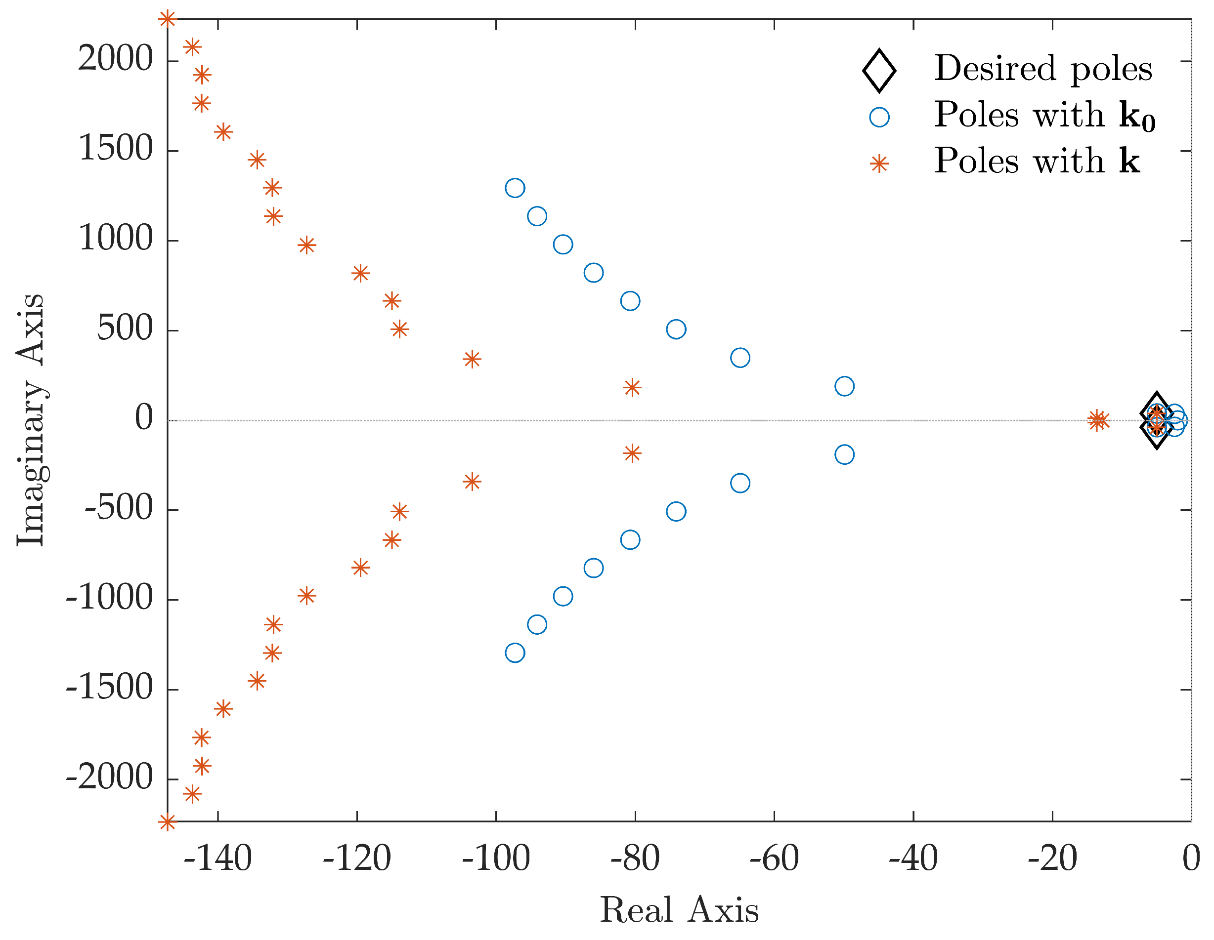
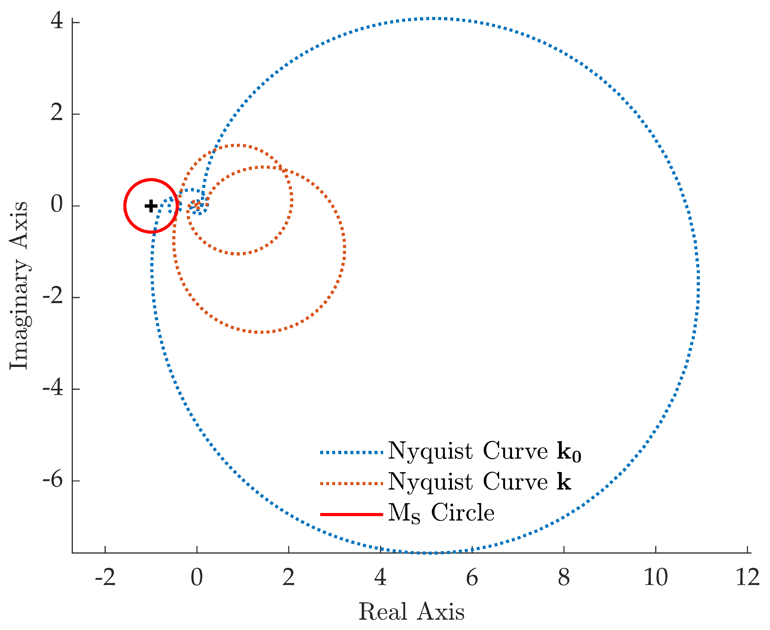
Pole placement is performed by computing the control gains through the receptance method proposed in Section 3.1, leading to and . The closed-loop poles are computed through the collection of Matlab functions released under the package DDE-Biftool [36] and are shown in Figure 3. The dominant closed-loop poles are summarized in Table 2, while the latent roots are omitted for brevity. The desired closed-loop poles are correctly assigned. Conversely, the closed-loop system Nyquist curve for the Loop Gain function shown in Figure 4 highlights that does not satisfy the prescribed robustness condition, since the Nyquist curve belongs to the circle.
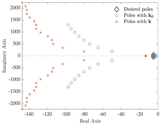
Figure 3.
Test case 1: closed-loop poles.
Table 2.
Test case 1: open-loop and closed-loop poles.

Figure 4.
Test case 1: Nyquist curve of .
The prescribed robustness is, in contrast, achieved by the method described in Section 3.2, that has led to the gain vector with and . The resulting closed-loop system features a Nyquist curve that does not belong to the circle for any complex value, as evidenced by Figure 4, and the desired poles are correctly assigned.
Note that neglecting the time delay in the synthesis of the controller, i.e., setting in Equation (8) and requiring the same two pairs of the primary closed-loop poles obtained through , leads to a control gain vector that destabilize the closed-loop system if these gains are applied to the time delayed system, due to the primary roots crossing the imaginary axis.
4.2.2. Test Case 2: Improving the Speed of Response
In the second example, the state feedback controller is tuned to modify the poles associated to the first vibrational mode. It is wanted to simultaneously increase its damping and its natural frequency, and hence the absolute values of both the real and the imaginary parts, to speed up the transient response. By means of example, the pair of poles is assigned to . Robustness is obtained by imposing .
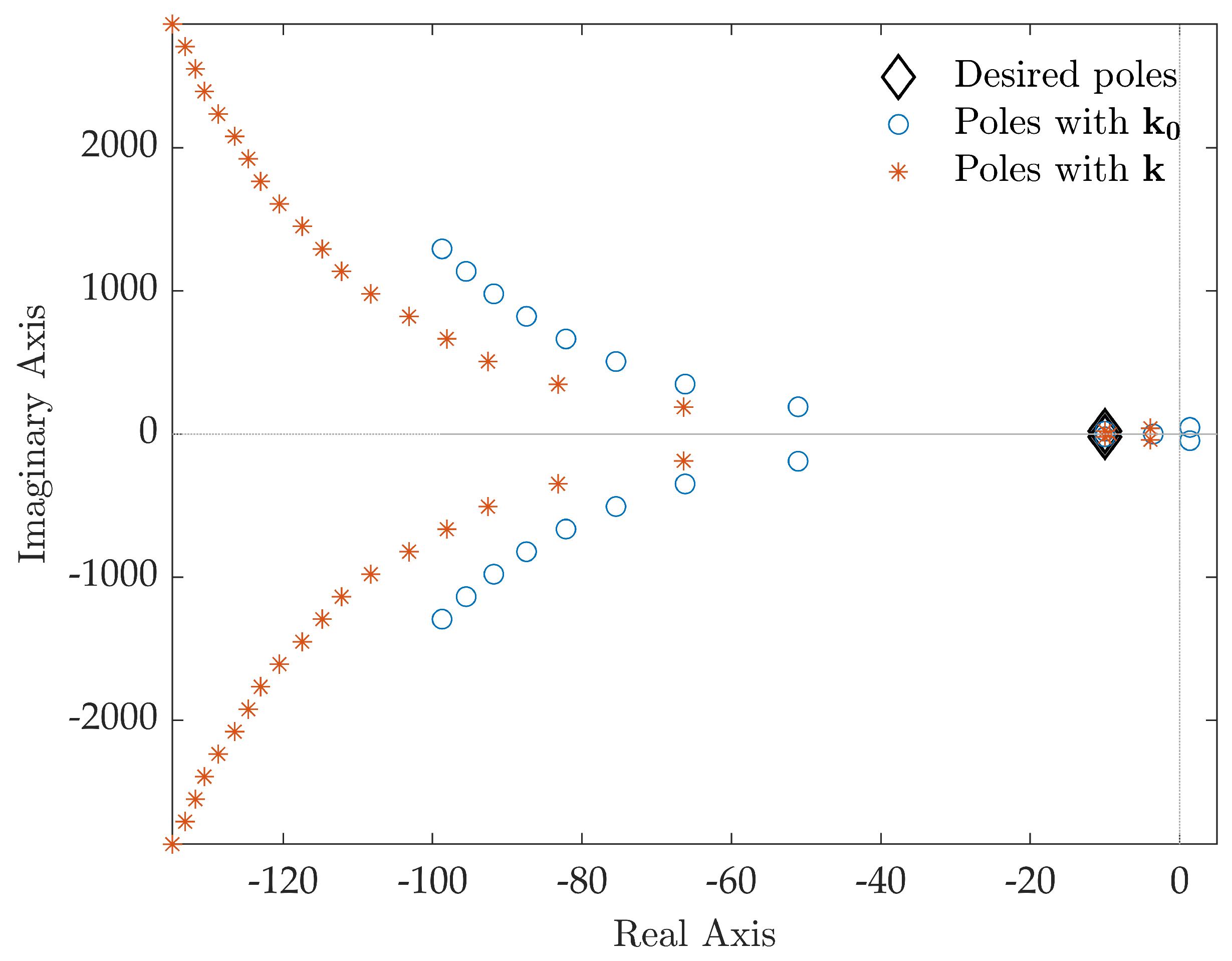
The pole placement task is correctly satisfied through , with and , obtained by solving Equation (8) through the function. In this case, as corroborated by the closed-loop poles listed in Table 3 and shown in Figure 5, the closed-loop system is unstable due to the spillover on the second pole pair that lies in the right-hand half of the complex plane.
Table 3.
Test case 2: open-loop and closed-loop poles.
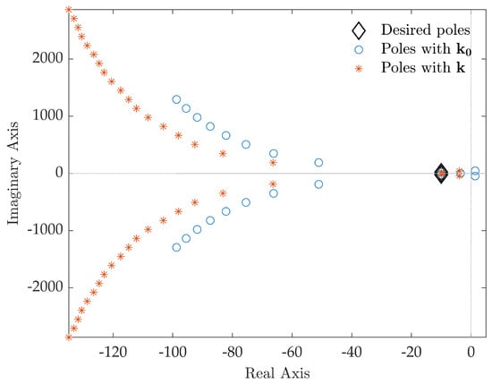
Figure 5.
Test case 2: closed-loop poles.
The method proposed in this paper tackles this problem by leading to , with and , that simultaneously satisfies the pole placement requirement and stabilizes the closed-loop system additionally ensuring the required robustness. The Nyquist curves of the loop gain of the closed-loop systems with and are shown in Figure 6 and clearly prove these aspects.
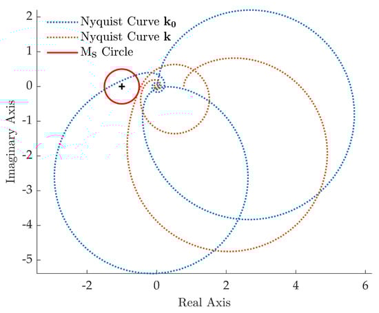
Figure 6.
Test case 2: Nyquist curve of .
4.3. Experimental Application
4.3.1. Application of the Controller of Test Case 1
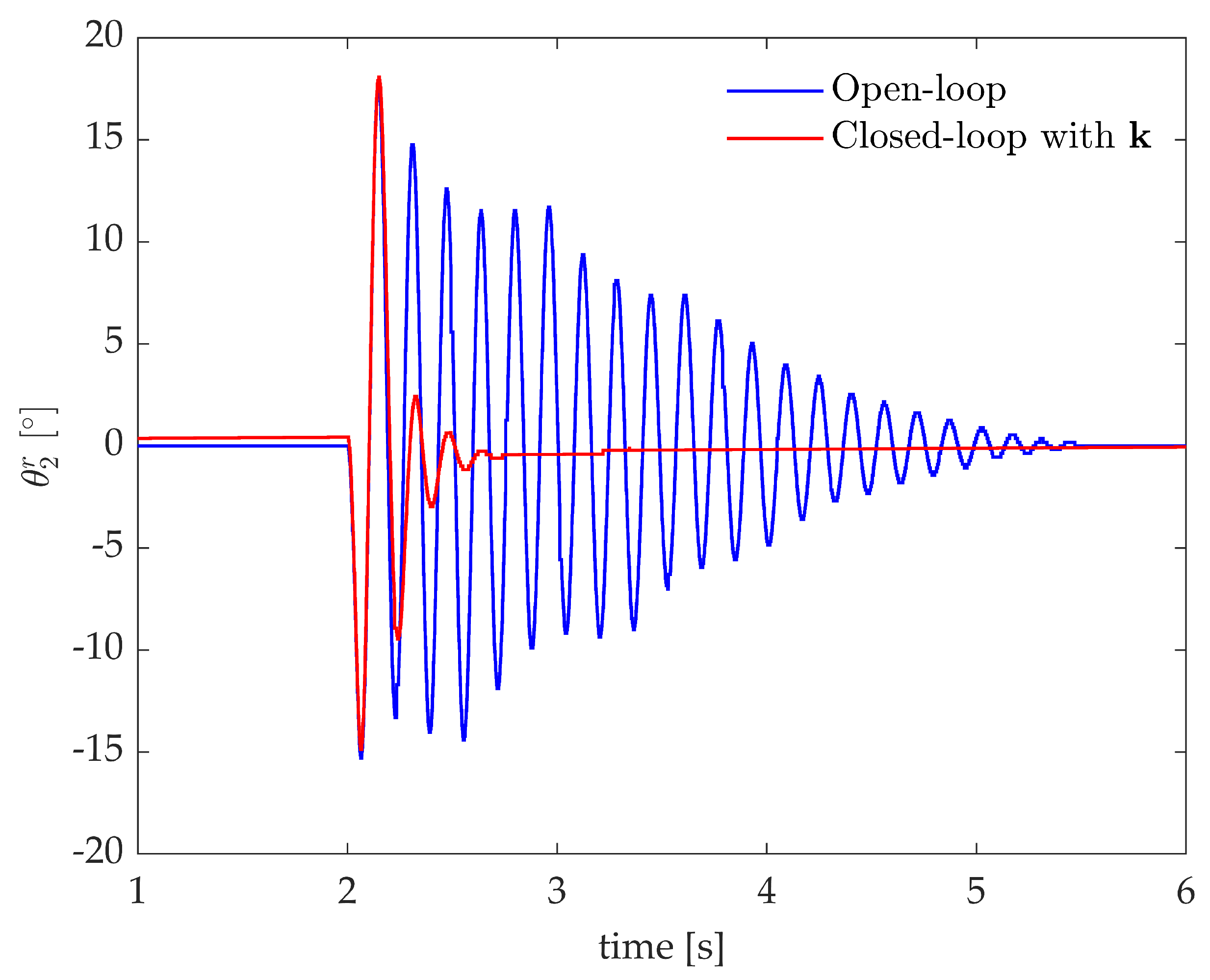
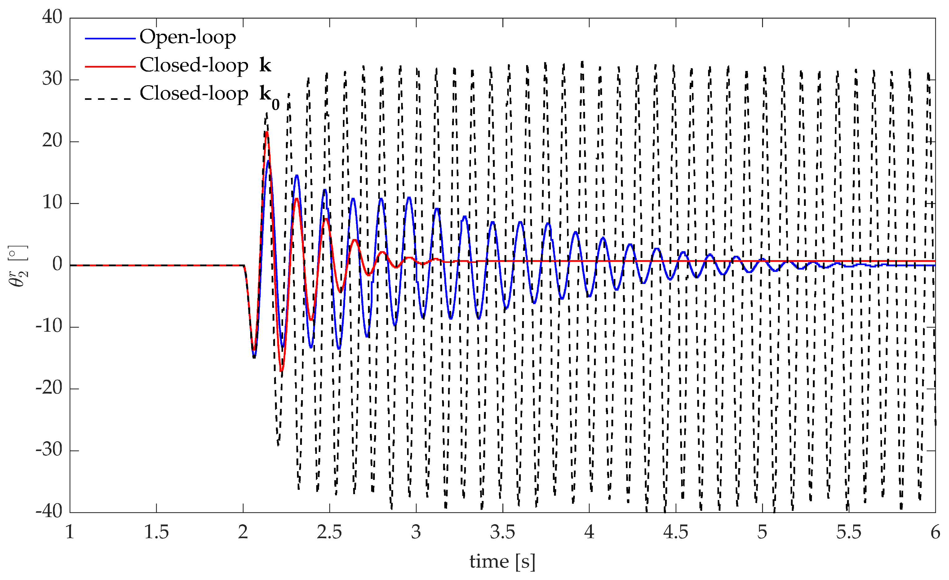
The controller proposed in Section 4.2.1 is applied to the experimental two-link flexible robot arm shown in Figure 2. An impulse-like torque disturbance is applied through the DC motor, the experimental responses of the open-loop and closed-loop system with are shown in Figure 7 through the relative angle of the second link .
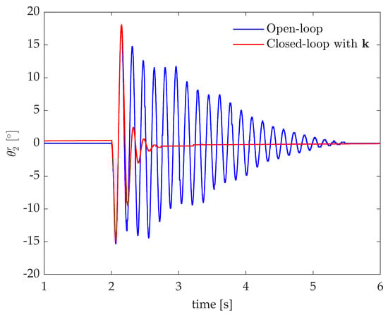
Figure 7.
Test case 1: experimental impulse responses, relative angle of the second-link.
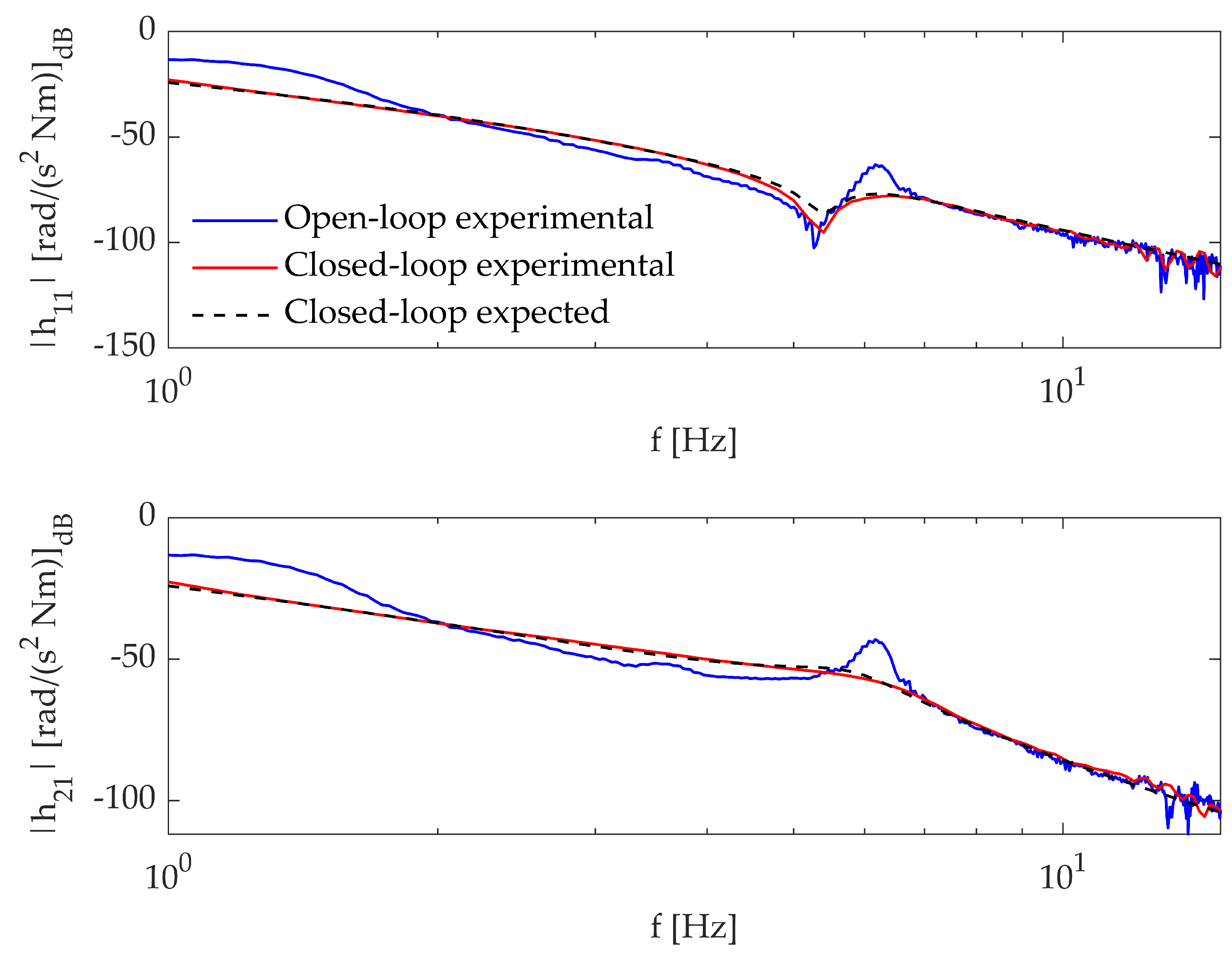
The modal parameters of the open-loop and closed-loop system are identified through the function and compared with the expected numerical counterpart in Table 4, where denotes the natural frequency and the related damping ratio. Additionally, the expected and experimental inertances for the open-loop and closed-loop system are shown in Figure 8. The fulfillment of the assignment task is evidenced by the agreement between the numerical data and the experimental measurements.
Table 4.
Test case 1: numerical and experimental modal parameters.

Figure 8.
Test case 1: expected and experimental inertances.
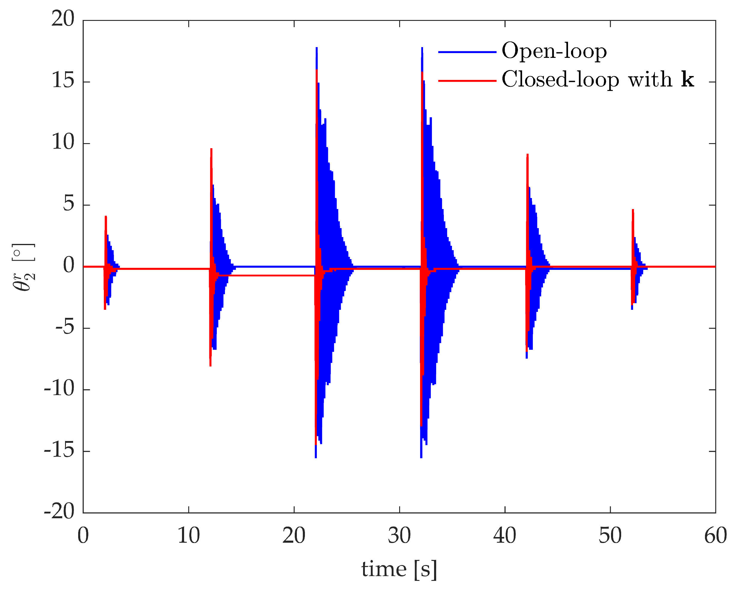
The agreement between the numerical expectations and the actual experimental results corroborates the controller robustness and its effectiveness to handle perturbations. Besides the linearization and the unavoidable, although small, errors on the measured receptances, the system is affected by the warp of the wire of encoder B that slightly perturbs the system mass distribution during the motion and also the equilibrium configuration. This effect is evident in Figure 9 where a train of pulses with different amplitudes is applied to obtain different nonlinear effects due to the geometrical non-linearity of the system (see Equation (13)). The motion of the wire causes slightly different equilibrium configurations once the response settles. Nonetheless, the controller ensures stable, fast, and repeatable vibration control, thus proving robustness.
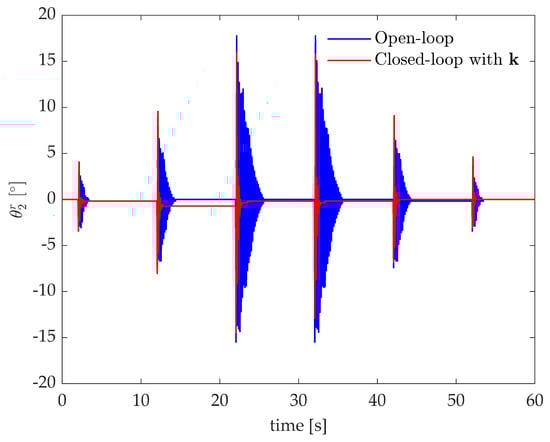
Figure 9.
Test case 1: experimental response to a train of impulses.
If no adequate robustness in obtained, the nominally stabilizing controller might result unstable or, at least, remarkably downgrade the actual performances. The robustness of the controller synthesized through the proposed method, i.e., the one with gains , is even more evident if it is compared with the non-robust controller tuned through . The experimental impulsive response of is shown in Figure 10.
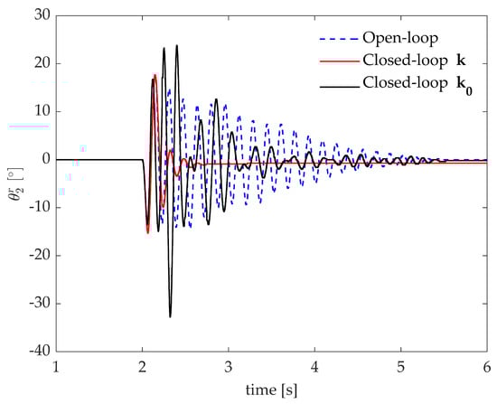
Figure 10.
Test case 1: experimental impulse response with the non-robust controller .
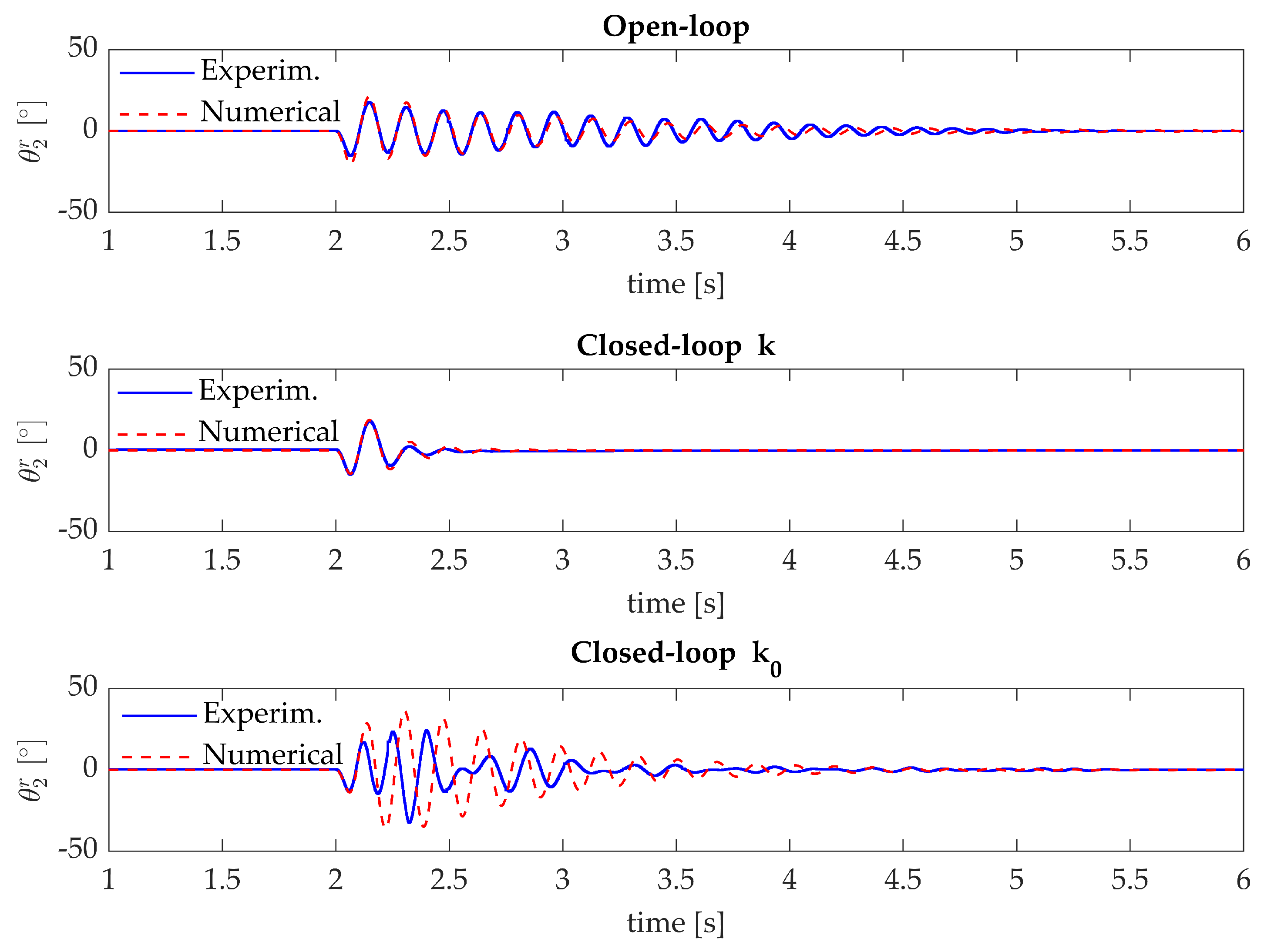
The numerical and experimental responses of the open-loop and closed-loop systems with and are compared in Figure 11. These provide a satisfying agreement for the open-loop and closed-loop system with , while in case of the experimental results do not match with the expected numerical results. It is evident that improving robustness is mandatory to enable for practical applications with adequate and reliable performances.
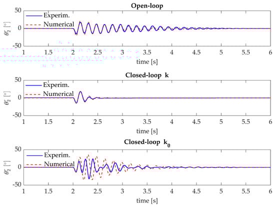
Figure 11.
Test case 1: comparison of the numerical and experimental open-loop and closed-loop impulse responses.
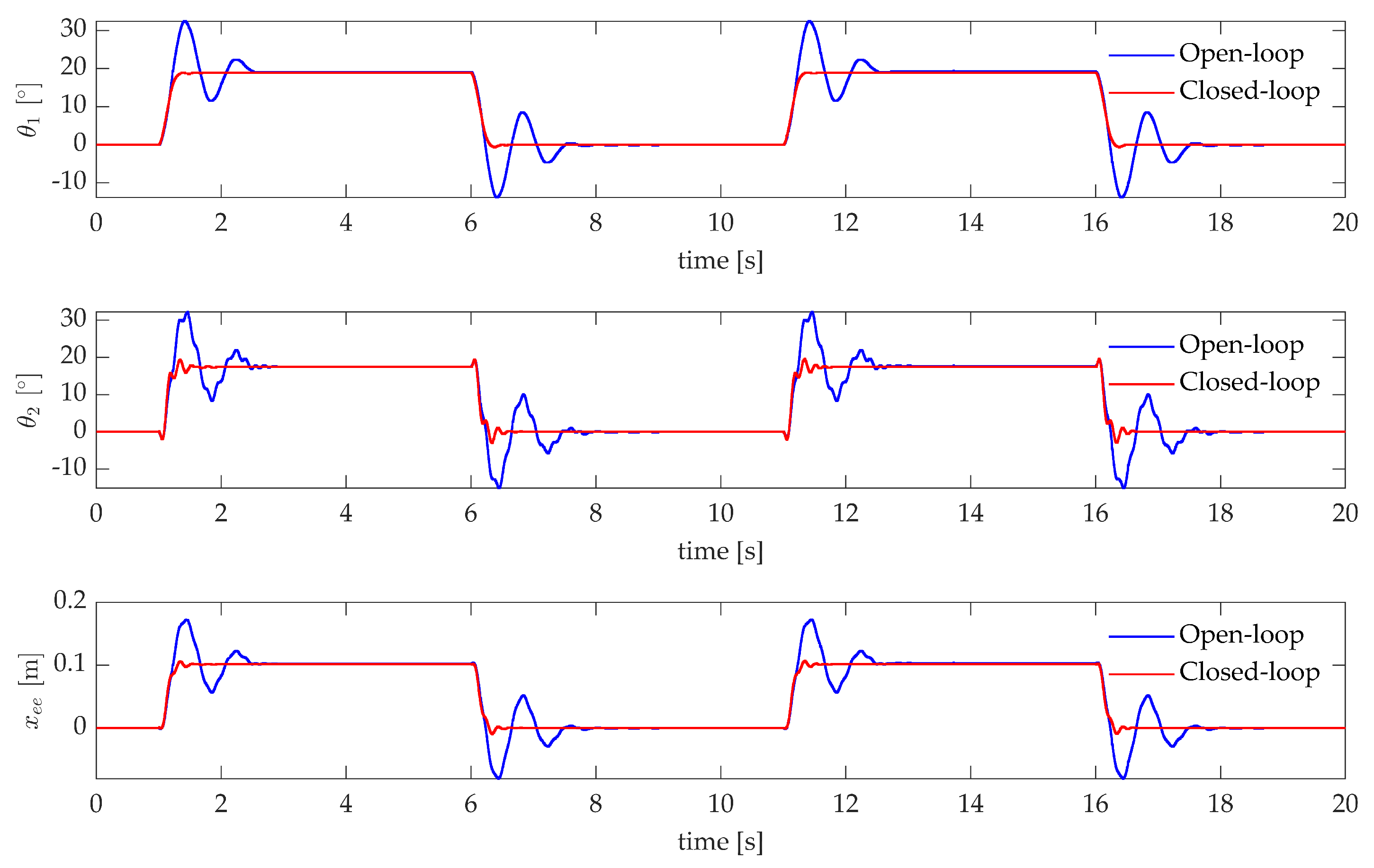
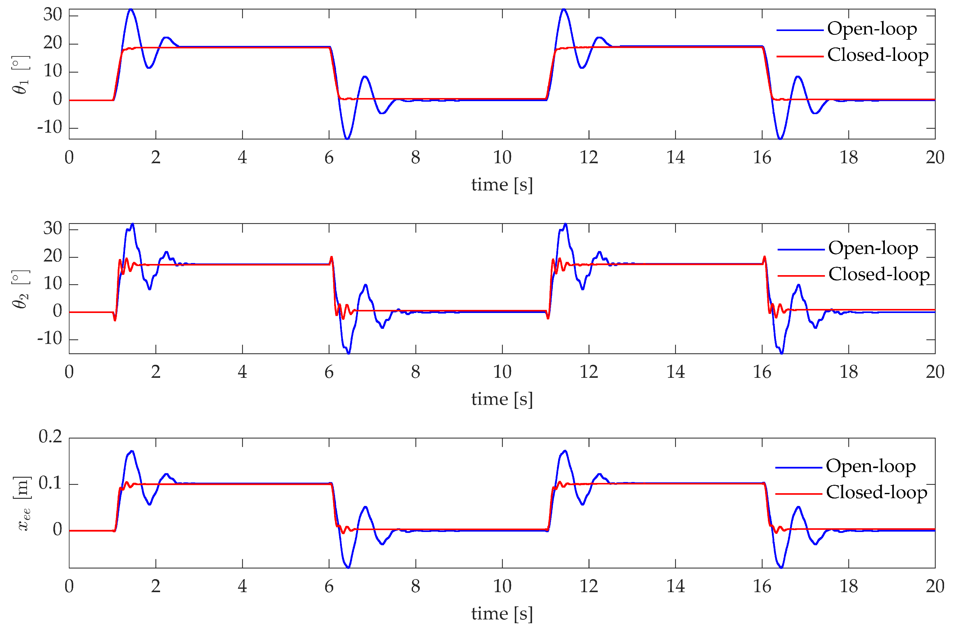
Last, Figure 12 shows the application of the controller to a step-tracking problem, that represents a typical pick-and-place task [37,38]. A sequence of step references to move the end-effector to the target value m is applied. The state-feedback controller is supported by a feedforward controller to compensate for gravity and friction and ensure no (or negligible) steady state error. Such feedforward control, that is the same for both the open and closed-loop schemes, consists of a square-wave, and does not affect the assigned closed-loop system eigenstructure. The comparison of the time responses, by denoting the 10–90% rise time and the 2% settling time is , shows that the controlled system fulfills the theoretical expectations. A faster response is exhibited (s and s) with respect to the open loop system (s and s), with just a negligible overshoot (, compared to the of the open loop system).
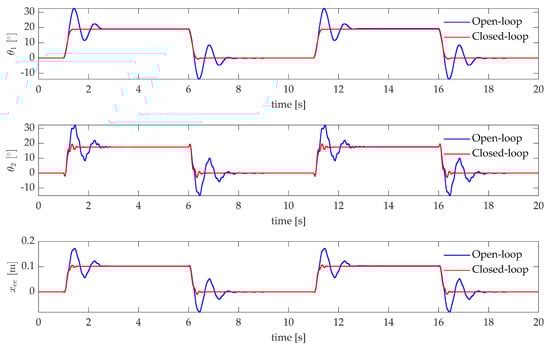
Figure 12.
Test case 1: experimental pick-and-place application.
4.3.2. Application of the Controller of Test Case 2
The controller designed in Section 4.2.2 is experimentally tested to assess its performances and robustness. The response to an impulse-like excitation exert by the DC motor is tested for the open-loop and the closed-loop systems with and . Figure 13 confirms that the controller tuned by solving Equation (8) (i.e., ) does not ensure asymptotic stability. Although a divergent behaviour in the case of was expected, oscillates between two bounded values due to the saturation of the exertable actuator torque (). In contrast, is stable, as expected, and ensures quick settling of the unwanted vibration. The natural frequency and damping of the closed-loop primary poles obtained with are compared with the expected numerical results in Table 5, and corroborate the correct fulfillment of the assignment task.
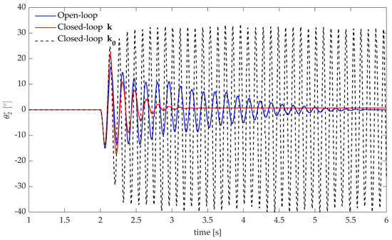
Figure 13.
Test case 2: experimental impulse response.
Table 5.
Test case 2: closed-loop numerical and experimental modal parameters.
The same controller is applied in the pick-and-place application discussed in Section 4.3.1. The experimental open-loop and closed-loop responses of the system are shown in Figure 14. The benefits of speeding up the first mode as done in test-case 2 (see Section 4.2.2) are evident. The second controller enables to simultaneously reduce the rise time and the settling time (s and s), with respect to both the open-loop and closed-loop system when the controller tuned to tackle the second mode is employed (see Section 4.2.1 and Section 4.3.1).
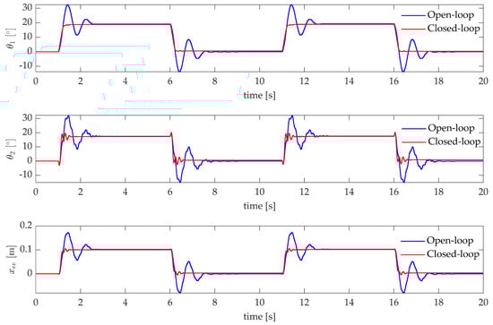
Figure 14.
Test case 2: experimental pick-and-place application.
5. Conclusions
This paper provides the experimental application of the method proposed by Araujo, Dantas, and Dorea for pole placement in flexible linear systems with time delay. The method exploits state feedback control to perform the partial pole placement of the desired system poles. The degrees of freedom in the choice of the control gains assigning such dominant poles is the leverage to stabilize all the remaining poles, including the infinite number of secondary roots due to the time delay, and to achieve the desired robustness of the closed-loop system. Robustness is quantified through the sensitivity function of the loop gain transfer function. The proposed technique exploits only the measured receptances, i.e., the system matrices , and are not needed to design the controller.
The effectiveness and usefulness of the proposed method is experimentally assessed against a challenging nonlinear and uncertain two-link flexible robot arm, whose flexibility arises due to the passive joint. Two controllers are tuned and experimentally applied to show different features of the method. The effectiveness of both controllers is evaluated by applying impulse disturbances as well a square wave reference (i.e., a sequence of steps) mimicking a pick-and-place robotic application. In both cases, the experimental application of the controllers provides excellent results and agreement with the expected numerical results. Besides effectively handling the severe time delays assumed, the imposed robustness allows the controller to get rid of the unavoidable uncertainties, e.g., due to the warp of the encoder wire, to the coarse encoder quantization, and to the nonlinear terms neglected in the controller design.
Due to the effectiveness of the proposed approach together with its simplicity, as a consequence of the use of the experimental receptances without the need of accurate system model, it is well suited for more complicated delayed systems such as mechatronic systems employed for manufacturing processes (see, e.g., in [3]), as well as robotic systems performing remote-operations [39] or teleoperations [40].
Author Contributions
Conceptualization, J.M.A., N.J.B.D., C.E.T.D., D.R., and I.T.; methodology, J.M.A., N.J.B.D., C.E.T.D., J.B., D.R., and I.T.; validation, J.B., D.R., and I.T.; formal analysis, J.M.A., N.J.B.D., J.B., D.R., and I.T.; investigation, J.M.A., N.J.B.D., J.B., D.R., and I.T.; software, J.M.A., N.J.B.D., J.B., and I.T.; resources, D.R.; data curation, I.T.; writing—original draft preparation, J.M.A., D.R., and I.T.; writing—review and editing, J.M.A., D.R., and I.T.; visualization, I.T.; supervision, J.M.A., C.E.T.D., and D.R.; project administration, J.M.A., C.E.T.D., and D.R.; funding acquisition, J.M.A., C.E.T.D., and D.R. All authors have read and agreed to the published version of the manuscript.
Funding
This research received no external funding.
Data Availability Statement
Data available on request.
Conflicts of Interest
The authors declare no conflict of interest.
References
- Ariyatanapol, R.; Xiong, Y.; Ouyang, H. Partial pole assignment with time delays for asymmetric systems. Acta Mech. 2018, 229, 2619–2629. [Google Scholar] [CrossRef] [Green Version]
- Sinou, J.; Chomette, B. Active vibration control and stability analysis of a time-delay system subjected to friction-induced vibration. J. Sound Vib. 2021, 500, 116013. [Google Scholar] [CrossRef]
- Olgac, N.; Sipahi, R. Dynamics and stability of variable-pitch milling. J. Vib. Control 2007, 13, 1031–1043. [Google Scholar] [CrossRef]
- Gu, K.; Niculescu, S.I. Survey on recent results in the stability and control of time-delay systems. J. Dyn. Sys. Meas. Control 2003, 125, 158–165. [Google Scholar] [CrossRef]
- Li, S.; Zhu, C.; Mao, Q.; Su, J.; Li, J. Active disturbance rejection vibration control for an all-clamped piezoelectric plate with delay. Control. Eng. Pract. 2021, 108, 104719. [Google Scholar] [CrossRef]
- Birs, I.; Muresan, C.; Nascu, I.; Ionescu, C. A survey of recent advances in fractional order control for time delay systems. IEEE Access 2019, 7, 30951–30965. [Google Scholar] [CrossRef]
- Shi, T.; Shi, P.; Wang, S. Robust sampled-data model predictive control for networked systems with time-varying delay. Int. J. Robust Nonlinear Control. 2019, 29, 1758–1768. [Google Scholar] [CrossRef]
- Wu, M.; Cheng, J.; Lu, C.; Chen, L.; Chen, X.; Cao, W.; Lai, X. Disturbance estimator and smith predictor-based active rejection of stick–slip vibrations in drill-string systems. Int. J. Syst. Sci. 2020, 51, 826–838. [Google Scholar] [CrossRef]
- Araujo, J.M.; Santos, T.L. Control of second-order asymmetric systems with time delay: Smith predictor approach. Mech. Syst. Signal Process. 2020, 137, 106355. [Google Scholar] [CrossRef]
- Natori, K.; Oboe, R.; Ohnishi, K. Stability analysis and practical design procedure of time delayed control systems with communication disturbance observer. IEEE Trans. Ind. Inform. 2008, 4, 185–197. [Google Scholar] [CrossRef]
- Natori, K.; Oboe, R.; Ohnishi, K. Robustness on model error of time delayed control systems with communication disturbance observer-Verification on an example constructed by double integration controlled object and PD controller. IEEJ Trans. Ind. Appl. 2008, 128. [Google Scholar] [CrossRef]
- Zhou, W.; Wang, Y.; Liang, Y. Sliding mode control for networked control systems: A brief survey. ISA Trans. 2021, in press. [Google Scholar] [CrossRef]
- Nian, F.; Shen, S.; Zhang, C.; Lv, G. Robust Switching Control for Force-reflecting Telerobotic with Time-varying Communication Delays. In Proceedings of the 2020 Chinese Control And Decision Conference (CCDC), Hefei, China, 21–23 May 2020; pp. 1714–1719. [Google Scholar]
- Kautsky, J.; Nichols, N.K.; Van Dooren, P. Robust pole assignment in linear state feedback. Int. J. Control. 1985, 41, 1129–1155. [Google Scholar] [CrossRef]
- Chu, E.; Datta, B. Numerically robust pole assignment for second-order systems. Int. J. Control. 1996, 64, 1113–1127. [Google Scholar] [CrossRef]
- Ram, Y.M.; Mottershead, J.E. Receptance method in active vibration control. AIAA J. 2007, 45, 562–567. [Google Scholar] [CrossRef]
- Ram, Y.; Singh, A.; Mottershead, J.E. State feedback control with time delay. Mech. Syst. Signal Process. 2009, 23, 1940–1945. [Google Scholar] [CrossRef]
- Ram, Y.; Mottershead, J.; Tehrani, M.G. Partial pole placement with time delay in structures using the receptance and the system matrices. Linear Algebra Its Appl. 2011, 434, 1689–1696. [Google Scholar] [CrossRef] [Green Version]
- Pratt, J.M.; Singh, K.V.; Datta, B.N. Quadratic partial eigenvalue assignment problem with time delay for active vibration control. J. Phys. Conf. Ser. 2009, 181, 012092. [Google Scholar] [CrossRef]
- Singh, K.V.; Dey, R.; Datta, B.N. Partial eigenvalue assignment and its stability in a time delayed system. Mech. Syst. Signal Process. 2014, 42, 247–257. [Google Scholar] [CrossRef]
- Belotti, R.; Richiedei, D. Pole assignment in vibrating systems with time delay: An approach embedding an a-priori stability condition based on Linear Matrix Inequality. Mech. Syst. Signal Process. 2020, 137, 106396. [Google Scholar] [CrossRef]
- Dantas, N.J.; Dorea, C.E.; Araujo, J.M. Partial pole assignment using rank-one control and receptance in second-order systems with time delay. Meccanica 2021, 56, 287–302. [Google Scholar] [CrossRef]
- De Luca, A.; Lucibello, P.; Ulivi, G. Inversion techniques for trajectory control of flexible robot arms. J. Robot. Syst. 1989, 6, 325–344. [Google Scholar] [CrossRef] [Green Version]
- Araújo, J.M. Discussion on ‘State feedback control with time delay’. Mech. Syst. Signal Process. 2018, 98, 368–370. [Google Scholar] [CrossRef]
- Sherman, J.; Morrison, W.J. Adjustment of an inverse matrix corresponding to a change in one element of a given matrix. Ann. Math. Stat. 1950, 21, 124–127. [Google Scholar] [CrossRef]
- Belotti, R.; Richiedei, D.; Tamellin, I.; Trevisani, A. Pole assignment for active vibration control of linear vibrating systems through linear matrix inequalities. Appl. Sci. 2020, 10, 5494. [Google Scholar] [CrossRef]
- Richiedei, D.; Tamellin, I. Active control of linear vibrating systems for antiresonance assignment with regional pole placement. J. Sound Vib. 2021, 494, 115858. [Google Scholar] [CrossRef]
- Astroem, K.J.; Murray, R.M. Feedback Systems: An Introduction for Scientists and Engineers, 2nd ed.; Princeton University Press: Princeton, NJ, USA, 2021. [Google Scholar]
- Skogestad, S.; Postlethwaite, I. Multivariable Feedback Control: Analysis and Design; Wiley: New York, NY, USA, 2007; Volume 2. [Google Scholar]
- Nyquist, H. Regeneration Theory. Bell Syst. Tech. J. 1932, 11, 126–147. [Google Scholar] [CrossRef]
- Seiler, P.; Packard, A.; Gahinet, P. An Introduction to Disk Margins [Lecture Notes]. IEEE Control. Syst. Mag. 2020, 40, 78–95. [Google Scholar] [CrossRef]
- Franklin, T.S.; Araújo, J.M.; Santos, T.L. Receptance-based robust stability criteria for second-order linear systems with time-varying delay and unstructured uncertainties. Mech. Syst. Signal Process. 2021, 149, 107191. [Google Scholar] [CrossRef]
- Zhao, X.; Li, Y.; Boonen, P. Intelligent optimization algorithm of non-convex function based on genetic algorithm. J. Intell. Fuzzy Syst. 2018, 35, 4289–4297. [Google Scholar] [CrossRef]
- Goldberg, D.E. Genetic Algorithms in Search, Optimization and Machine Learning, 1st ed.; Addison-Wesley Longman Publishing Co., Inc.: Boston, MA, USA, 1989. [Google Scholar]
- Richiedei, D.; Trevisani, A. Simultaneous active and passive control for eigenstructure assignment in lightly damped systems. Mech. Syst. Signal Process. 2017, 85, 556–566. [Google Scholar] [CrossRef]
- Engelborghs, K.; Luzyanina, T.; Roose, D. Numerical bifurcation analysis of delay differential equations using DDE-BIFTOOL. ACM Trans. Math. Softw. 2002, 28, 1–21. [Google Scholar] [CrossRef]
- Choi, S.B.; Seong, M.S.; Ha, S.H. Accurate position control of a flexible arm using a piezoactuator associated with a hysteresis compensator. Smart Mater. Struct. 2013, 22, 045009. [Google Scholar] [CrossRef]
- Scalera, L.; Boscariol, P.; Carabin, G.; Vidoni, R.; Gasparetto, A. Enhancing energy efficiency of a 4-DOF parallel robot through task-related analysis. Machines 2020, 8, 10. [Google Scholar] [CrossRef] [Green Version]
- Vaughan, J.; Peng, K.C.C.; Singhose, W.; Seering, W. Influence of remote-operation time delay on crane operator performance. IFAC Proc. Vol. 2012, 45, 85–90. [Google Scholar] [CrossRef]
- Slama, T.; Trevisani, A.; Aubry, D.; Oboe, R.; Kratz, F. Experimental analysis of an internet-based bilateral teleoperation system with motion and force scaling using a model predictive controller. IEEE Trans. Ind. Electron. 2008, 55, 3290–3299. [Google Scholar] [CrossRef]


Publisher’s Note: MDPI stays neutral with regard to jurisdictional claims in published maps and institutional affiliations. |
© 2021 by the authors. Licensee MDPI, Basel, Switzerland. This article is an open access article distributed under the terms and conditions of the Creative Commons Attribution (CC BY) license (https://creativecommons.org/licenses/by/4.0/).