Nonlinear Suppression of a Dual-Tube Coriolis Mass Flowmeter Based on Synchronization Effect

Featured Application

1. Investigated an additional-mass method to suppress the nonlinear frequency doubling phenomenon; 2. established a coupling system vibration model with additional mass; 3. determined the suppression effect of the additional mass on the nonlinear frequency doubling phenomenon, and experimentally verified the CMF; 4. the conclusions of this study have certain guiding significance for the suppression of the nonlinear frequency doubling phenomenon of flowmeters in actual industrial production.

Abstract

Nonlinear interference components exist in the output signals of dual-tube Coriolis mass flowmeters (CMFs) which affect the sensitivity and accuracy of the devices. This nonlinearity still appears under zero flow, which is manifested when the output signal contains a frequency doubling signal. This study (1) investigated an additional-mass method to suppress the nonlinear frequency doubling phenomenon, (2) established a coupling system vibration model with additional mass, built a dynamic differential equation for the vibration of the double-beam coupling system from the Lagrange equation, (3) obtained amplitude frequency information using a fourth-order Runge–Kutta method, (4) determined the suppression effect of the additional mass on the nonlinear frequency doubling phenomenon, and (5) experimentally verified the CMF. The results showed that the base coupled the vibrations of two beams, and the symmetric additional mass suppressed the nonlinear frequency doubling phenomenon, thus suppressing low or high frequencies. Also, the effect of pipeline defects simulated under asymmetric additional mass was obtained through numerical analysis and experimental data. Flowmeters with a required measuring frequency range had the optimal suppression effect on nonlinear frequency doubling and provided theoretical guidance for the nondestructive testing of measuring tubes.

1. Introduction

Resonator sensors are currently one of the best-performing types of sensors worldwide. A traditional resonator sensor is a linear system, but nonlinear interference components exist in the actual output signal. Taking a resonant Coriolis mass flowmeter (CMF) as an example, the excitation signal from the sensor is a single sinusoidal signal, and the detection signal of the sensor exists in the form of a nonlinear signal characterized by a frequency doubling signal [1,2].

To trace the nonlinear phenomenon of a CMF, many studies have analyzed the fluid properties [3], fluid-structure interaction [4,5], key parameters [6], and installation effects [7,8] of measuring tubes, nonideal boundary conditions [9,10,11], defects resulting from structural inhomogeneity [12,13], etc. At the same time, this phenomenon has also been observed in microfluidics; Maide Bucolo et al. [14,15] took advantage of the optical monitoring of slug flow in microchannels to characterize flow nonlinearity with rich and specific experiments. It is possible to distinguish clearly the air and water passages in the optical signal. The observation shows that there appear to be some frequency doubling signals in the spectrum.

However, the fundamental reasons for the nonlinear frequency doubling phenomenon of the absolute perfect CMF under zero flow conditions are rarely reported. Zero flow includes several situations: the fluid in the pipe is low-velocity fluid or a micro flow, the fluid fills the pipe and moves along the pipe at a uniform speed, or the fluid in the pipe is a gas. Synchronization generally takes place in two or more coupled and nonlinear autonomous oscillation systems of similar size. Synchronization is a fundamental theme in nonlinear phenomena and is a currently popular topic of research in the control field [16]. The earliest scientific description of synchronization dates back to 1665. The Dutch physicist Huygens found that two different pendulum clocks hanging on the wall swung in opposite directions, and gave the reason for the synchronous swing as being the coupled beams that the two clocks hung from interacted with each other so that the two clocks became fully synchronized after swinging for a period of time. This experimental device is shown in Figure 1 [17,18].

Following in Huygens’ footsteps, experimental research was begun on vibration-coupled pendulums, which were later replaced by modern rhythm clocks and mechanical metronomes. K. Czolczynski et al. fully replicated Huygens’ pendulum experiment, explored the effect of nonidentical pendulums, and explained synchronous behaviours under different coupling modes [19]. Wu Y et al. investigated the in-phase and antiphase synchronization phenomena of two coupled mechanical metronomes under random initial conditions [20]. Xin X analyzed the synchronization phenomenon of two metronome systems hanging on a cart, based on a description of the function method [21]. In summary, the synchronization problem of two or more same-frequency vibration sources in a system can be explained and solved based on the synchronization phenomenon. The system model is a typical nonlinear model, and the synchronization phenomenon induces nonlinear vibration coupling of the system.

Figure 2 is a structure diagram of a typical dual-tube CMF; its sensitive unit is a pair of completely symmetrical measuring tubes. When the measuring tubes are empty, a first-order bending vibration is invoked under the driving force of the exciting coil, and the measuring tube is in first-order resonance. The vibration of this U tube can be deemed as a circular motion around a fixed axis from a certain perspective. In reality, two symmetric sensitive units synchronously vibrate in a reverse direction under the action of the exciting unit, which is regarded as a typical antiphase synchronous motion. Based on synchronization theory and through numerical analysis, it has been confirmed that a nonlinear signal for the frequency doubling phenomenon really existed on Huygens’ double beams with coupled vibration [22].

Based on the coupled vibration induced by the synchronization phenomenon, this study further investigated the effect of additional mass on a coupling system vibration. Section 2 of this paper describes a coupled vibration model of the dual-tube model with additional mass, solves the differential equations for coupled vibration, and verifies the nonlinear frequency doubling phenomenon. Section 3 and Section 4 describe the effect of additional mass on the nonlinearity, which was determined by numerically solving the magnitude of additional mass and the distance away from the base and the position. Section 4 describes the experimental study of the specific dual-tube CMF and summarises the law, thus providing experimental bases and guidance for accurately suppressing the nonlinearity.

2. Nonlinear Analysis on Coupled Vibration of Dual-Tube Model with Additional Mass

Frequency is the most fundamental characteristic value in characterizing variations in structural properties, and the frequency of a real engineering structure is the most accessible modal parameter with high measurement accuracy [23,24]. It has been determined through previous theoretical analysis [22] that the nonlinearity invoked by the coupling effect cannot be fundamentally eliminated and is suppressed by changing the wall thickness and the mass and spacing of the measuring tube, among other structural parameters. However, once the mass of the measuring tube changes, the working frequency of the measuring tube inevitably changes. That affects the CMF performance such as measuring range and measuring accuracy and incurs higher manufacturing costs; if the CMF structure size changes, its installation conditions and working environment are affected, bringing inconvenient in use.

The additional-mass method is the most commonly used method for nondestructive testing of beam structures. The effects on the key structural parameters of a CMF, such as its mass and size, can be minimized by the additional-mass method, and some correlation exists between additional mass and structural modal parameters. Therefore, a very small additional mass relative to the entire mass has little effect on the original working frequency and measuring range of the CMF. By changing the magnitude and distribution of the additional mass, the law of nonlinearity suppression can be quickly obtained, and the best suppression position can be determined, thus greatly improving the CMF measuring accuracy.

Here, the CMF can be simplified to the abstract model shown in Figure 3, where $z_1,z_2,$and $z$ are the vibration displacement of the beams in its own coordinate system and system displacement;$m_1,m_2,$and $m$ are the masses of the beams and base, respectively; $F_1,F_2$ are the driving force of the exciting coil on the middle point of the flow tube are the equal harmonic driving force in an opposite direction; $EI$ is the flexural rigidity of cantilever beam $i$, and ${\xi }_i$ indicates the position coordinates of the additional mass $m_{oi}$of the coupling system on the beams.

The coupled vibration model of the dual-tube model with additional mass was built, and the generalized coordinates were defined as $q=\left(q_{1i},q_{2i},\dots ,q_{ji},z\right)$.$z_i\left(x,t\right)$ is the transverse vibration displacement function of cantilever beam$i$. According to the modal superposition method,$z_i\left(x,t\right)$ can be depicted as the superposition form of each order of modal, and single beam$i$ has the following form:

$$z_i\left(x,t\right)\approx {{\displaystyle \sum }}_{j=1}^n{\varphi }_{ji}\left(x\right)q_{ji}\left(t\right)$$

(1)

where ${\varphi }_{ji}\left(x\right)$ is the $j^{\mathrm{th}}$ order vibration mode of beam $i$ with additional mass, and $q_{ji}\left(t\right)$ is a generalized coordinate and only time-dependent. $j$ is the$j^{\mathrm{th}}$ order modal. Here, the first three orders were chosen for analysis. Next, the motion differential equation of the system was obtained by constructing a Lagrange equation of the following general form:

$$\frac{d}{dt}\left\{\frac{\partial \left(T-U-U_k\right)}{\partial {\dot{q}}_j}\right\}-\frac{\partial \left(T-U-U_k\right)}{\partial q_j}=Q_r$$

(2)

The generalized force at the right end of the equation is

$$Q_z=-C\frac{\partial z\left(t\right)}{\partial t}$$

(3)

$$Q_{z_i}=F_i\delta \left(x-l\right)$$

(4)

Based on the small deformation theory, the deformation energy of the beams in the system under transverse bending has the following form:

$$U=\frac{1}{2EI}{{\displaystyle \int }}_0^l{\left[M\left(x\right)\right]}^{2}dx=\frac{EI}{2}{{\displaystyle \int }}_0^l\left[{\left(\frac{{\partial }^2{Z}_{11}\left(x,t\right)}{\partial x^2}\right)}^2+{\left(\frac{{\partial }^2{Z}_{12}\left(x,t\right)}{\partial x^2}\right)}^2\right]dx$$

(5)

Figure 3 shows that the CMF base was simplified to a single-degree-of-freedom spring damper system, such that the potential energy of the base is a spring elastic potential energy:

$$U_k=\frac{1}{2}kz{\left(t\right)}^2.$$

(6)

The kinetic energy of the entire system is added, and the kinetic energy of additional mass is related to the position and magnitude of additional mass. The total kinetic energy is expressed as

$$T=\frac{1}{2}m{\left(\frac{\partial z\left(t\right)}{\partial t}\right)}^2+\frac{1}{2}\frac{m_1}{l}{{\displaystyle \int }}_0^l{\left(\frac{\partial z\left(t\right)}{\partial t}-\frac{\partial z_{11}\left(x,t\right)}{\partial t}\right)}^{2}dx+\frac{1}{2}\frac{m_2}{l}{{\displaystyle \int }}_0^l{\left(\frac{\partial z\left(t\right)}{\partial t}-\frac{\partial z_{12}\left(x,t\right)}{\partial t}\right)}^{2}dx+\frac{1}{2}{m}_{01}{\left(\frac{\partial z\left(t\right)}{\partial t}-\frac{\partial Z_{11}\left({\xi }_1,t\right)}{\partial t}\right)}^2+\frac{1}{2}{m}_{02}{\left(\frac{\partial z\left(t\right)}{\partial t}-\frac{\partial Z_{12}\left({\xi }_2,t\right)}{\partial t}\right)}^2$$

(7)

The different generalized coordinates are calculated as follows:

(1)

Generalized coordinate $q_{1i}$

$$\frac{d}{dt}\left\{\frac{\partial \left(T-U-U_k\right)}{\partial {\dot{q}}_{1i}}\right\}=\frac{m_i}{l}{{\displaystyle \int }}_0^l\left[-{\varphi }_{1i}\left(x\right)\frac{{\partial }^{2}z\left(t\right)}{\partial t^2}+{\left({\varphi }_{1i}\left(x\right)\right)}^2\frac{{\partial }^2{q}_{1i}\left(t\right)}{\partial t^2}\right]dx+m_{oi}\left[-{\varphi }_{1i}\left({\xi }_i\right)\frac{{\partial }^{2}z\left(t\right)}{\partial t^2}+{\left({\varphi }_{1i}\left({\xi }_i\right)\right)}^2\frac{{\partial }^2{q}_{1i}\left(t\right)}{\partial t^2}\right]$$

(8)

$$\frac{\partial \left(T-U-U_k\right)}{\partial q_{1i}}=-\frac{\partial \left({{\displaystyle \sum }}_1^2\frac{EI}{2}{{\displaystyle \int }}_0^l{\left(\frac{{\partial }^2{\varphi }_{1i}\left(x\right)q_{1i}\left(t\right)}{\partial x^2}\right)}^{2}dx\right)}{\partial q_{1i}}=-EI{q}_{1i}\left(t\right){{\displaystyle \int }}_0^l{\left(\frac{{\partial }^2{\varphi }_{1i}\left(x\right)}{\partial x^2}\right)}^{2}dx$$

(9)

By substituting Equations (8) and (9) into Equation (2), the following differential equation can be obtained:

$$\frac{m_i}{l}{{\displaystyle \int }}_0^l\left[-{\varphi }_{1i}\left(x\right)\frac{{\partial }^{2}z\left(t\right)}{\partial t^2}+{\left({\varphi }_{1i}\left(x\right)\right)}^2\frac{{\partial }^2{q}_{1i}\left(t\right)}{\partial t^2}\right]dx+m_{oi}\left[-{\varphi }_{1i}\left({\xi }_i\right)\frac{{\partial }^{2}z\left(t\right)}{\partial t^2}+{\left({\varphi }_{1i}\left({\xi }_i\right)\right)}^2\frac{{\partial }^2{q}_{1i}\left(t\right)}{\partial t^2}\right]+EI{q}_{1i}\left(t\right){{\displaystyle \int }}_0^l{\left(\frac{{\partial }^2{\varphi }_{1i}\left(x\right)}{\partial x^2}\right)}^{2}dx=F_i\left(t\right)$$

(10)

(2)

Generalized coordinate$z$

$$\frac{d}{dt}\left\{\frac{\partial \left(T-U-U_k\right)}{\partial \dot{z}}\right\}=\left(m+m_1+m_2+m_{o1}+m_{o2}\right)\frac{{\partial }^{2}z\left(t\right)}{\partial t^2}-{{\displaystyle \sum }}_{i=1}^2\frac{m_i}{l}{{\displaystyle \int }}_0^l{\varphi }_{1i}\left(x\right)\left(\frac{{\partial }^2{q}_{1i}\left(t\right)}{\partial t^2}\right)dx+{{\displaystyle \sum }}_{i=1}^2{m}_{oi}\left[\frac{{\partial }^{2}z\left(t\right)}{\partial t^2}-{\varphi }_{1i}\left({\xi }_i\right)\frac{{\partial }^2{q}_{1i}\left(t\right)}{\partial t^2}\right]$$

(11)

$$\frac{\partial \left(T-U-U_k\right)}{\partial z}=-kz$$

(12)

By substituting Equations (11) and (12) into Equation (2), the motion differential equation can be obtained as follows:

$$\left(m+m_1+m_2+m_{o1}+m_{o2}\right)\frac{{\partial }^{2}z\left(t\right)}{\partial t^2}-{{\displaystyle \sum }}_{i=1}^2\frac{m_i}{l}{{\displaystyle \int }}_0^l{\varphi }_{1i}\left(x\right)\left(\frac{{\partial }^2{q}_{1i}\left(t\right)}{\partial t^2}\right)dx+{{\displaystyle \sum }}_{i=1}^2{m}_{oi}\left[\frac{{\partial }^{2}z\left(t\right)}{\partial t^2}-{\varphi }_{1i}\left({\xi }_i\right)\frac{{\partial }^2{q}_{1i}\left(t\right)}{\partial t^2}\right]+kz=-C\frac{\partial z\left(t\right)}{\partial t}$$

(13)

The above equations together make up the system differential equation, where the physical parameters and the vibration functions are known, so this differential equation is solvable.

The dynamic differential equation of the double-beam coupled vibration model has the following form:

$$\{\begin{array}{c}\frac{m_i}{l}{{\displaystyle \int }}_0^l\left[-{\varphi }_{1i}\left(x\right)\frac{{\partial }^{2}z\left(t\right)}{\partial t^2}+{\left({\varphi }_{1i}\left(x\right)\right)}^2\frac{{\partial }^2{q}_{1i}\left(t\right)}{\partial t^2}\right]dx+m_{oi}\left[-{\varphi }_{1i}\left({\xi }_i\right)\frac{{\partial }^{2}z\left(t\right)}{\partial t^2}+{\left({\varphi }_{1i}\left({\xi }_i\right)\right)}^2\frac{{\partial }^2{q}_{1i}\left(t\right)}{\partial t^2}\right]\\ +EI{q}_{1i}\left(t\right){{\displaystyle \int }}_0^l{\left(\frac{{\partial }^2{\varphi }_{1i}\left(x\right)}{\partial x^2}\right)}^{2}dx=F_i\left(t\right)\\ \left(m+m_1+m_2+m_{o1}+m_{o2}\right)\frac{{\partial }^{2}z\left(t\right)}{\partial t^2}-{\displaystyle {\displaystyle \sum }_{i=1}^2}\frac{m_i}{l}{{\displaystyle \int }}_0^l{\varphi }_{1i}\left(x\right)\left(\frac{{\partial }^2{q}_{1i}\left(t\right)}{\partial t^2}\right)dx\\ +{\displaystyle {\displaystyle \sum }_{i=1}^2}{m}_{oi}\left[\frac{{\partial }^{2}z\left(t\right)}{\partial t^2}-{\varphi }_{1i}\left({\xi }_i\right)\frac{{\partial }^2{q}_{1i}\left(t\right)}{\partial t^2}\right]+kz=-C\frac{\partial z\left(t\right)}{\partial t}\end{array}$$

(14)

The equation is simplified as

$${{\displaystyle \int }}_0^l{\varphi }_{1i}\left(x\right)dx=W_{1i}$$

(15)

$${{\displaystyle \int }}_0^l{\varphi }_{1i}^2\left(x\right)dx=W_{2i}$$

(16)

$${{\displaystyle \int }}_0^l{\left(\frac{{\partial }^2{\varphi }_{1i}\left(x\right)}{\partial x^2}\right)}^{2}dx=W_{3i}$$

(17)

Thus, Equation (14) can be written as

$$\{\begin{array}{c}\rho A\left[-W_{1i}\frac{{\partial }^{2}z\left(t\right)}{\partial t^2}+W_{2i}\frac{{\partial }^2{q}_{1i}\left(t\right)}{\partial t^2}\right]+m_{oi}\left[-{\varphi }_{1i}\left({\xi }_i\right)\frac{{\partial }^{2}z\left(t\right)}{\partial t^2}+{\left({\varphi }_{1i}\left({\xi }_i\right)\right)}^2\frac{{\partial }^2{q}_{1i}\left(t\right)}{\partial t^2}\right]+EI{q}_{1i}\left(t\right)W_{3i}=F_i\left(t\right)\\ \left(m+m_1+m_2+m_{o1}+m_{o2}\right)\frac{{\partial }^{2}z\left(t\right)}{\partial t^2}-W_{1i}{\displaystyle {\displaystyle \sum }_{i-1}^2}\rho A\frac{{\partial }^2{q}_{1i}\left(t\right)}{\partial t^2}+{\displaystyle {\displaystyle \sum }_{i=1}^2}{m}_{oi}\left[\frac{{\partial }^{2}z\left(t\right)}{\partial t^2}-{\varphi }_{1i}\left({\xi }_i\right)\frac{{\partial }^2{q}_{1i}\left(t\right)}{\partial t^2}\right]+kz+c\frac{\partial z\left(t\right)}{\partial t}=0\end{array}$$

(18)

Equation (18) shows that regardless of whether additional mass is added, higher differentiation exists, and it is also a nonlinear ordinary differential equation. Previous analysis has found that if no accessory mass exists, a significant odd-numbered frequency doubling phenomenon is observed in the frequency domain diagram, which confirms the existence of the frequency doubling phenomenon on double beams with coupled vibration [22]. However, as determined by previous studies, nonlinear phenomena cannot be suppressed by changing the local mass, so the specific value was solved by Equation (18).

3. Numerical Solution and Analysis

Here, fourth order Runge–Kutta methods were used as numerical solution methods. By reducing the order of the equations, the numerical solution method is applicable to the equations with high-order differentials. Given

$$z=y_1,\frac{\partial z\left(t\right)}{\partial t}=y_2,q_{11}=y_3,\frac{\partial q_{11}\left(t\right)}{\partial t}=y_4,q_{12}=y_5,\frac{\partial q_{12}\left(t\right)}{\partial t}=y_6$$

(19)

The differential equations are simplified to the following form:

$$\{\begin{array}{c}{y}_2=\dot{y_1}\\ y_4=\dot{y_3}\\ y_6=\dot{y_5}\\ \rho A\left[-W_{11}\dot{y_2}+W_{21}\dot{y_4}\right]+m_{o1}\left[-{\varphi }_{11}\left({\xi }_1\right)\dot{y_2}+{\left({\varphi }_{11}\left({\xi }_1\right)\right)}^2\dot{y_4}\right]+EI{W}_{31}{y}_3=F_1\left(t\right)\\ \rho A\left[-W_{12}\dot{y_2}+W_{22}\dot{y_6}\right]+m_{o2}\left[-{\varphi }_{12}\left({\xi }_2\right)\dot{y_2}+{\left({\varphi }_{12}\left({\xi }_2\right)\right)}^2\dot{y_6}\right]+EI{W}_{32}{y}_5=F_2\left(t\right)\\ \left(m+m_1+m_2+m_{o1}+m_{o2}\right)\dot{y_2}-W_{11}\rho A\dot{y_4}-W_{12}\rho A\dot{y_6}+m_{o1}\left[\dot{y_2}-{\varphi }_{11}\left({\xi }_1\right)\dot{y_4}\right]+m_{o2}\left[\dot{y_2}-{\varphi }_{12}\left({\xi }_2\right)\dot{y_6}\right]+k{y}_1+c{y}_2=0\end{array}$$

(20)

3.1. No Additional Mass

In accordance with the actual CMF parameters, the parameters of the coupling tubes were designed as shown in

Table 1. Parameters of measuring tube.

Parameter	Value
Length of single beam	0.232 m
Diameter of single beam	0.01 m
Density	7890 kg/${\mathrm{m}}^3$
Base mass	3 kg
Elastic modulus	206 GPa

. Using MATLAB, $y_3$and $y_5$ were numerically solved by the Runge–Kutta methods. Given that $y=y_3-y_5$, a series of points for $y$ numerical solutions were obtained. After a fast Fourier transform, the response spectrogram of the double-beam coupled vibration system was finally obtained, as shown in Figure 4.

Figure 4 and the table in the figure show that the first-order natural frequency (Ω₁ = 132.64 Hz) and the obvious frequency doubling components found in the spectrogram corresponded to 3(Ω₂ = 397.77 Hz), 5(Ω₃ = 663.06 Hz) times, which has been mentioned in previous studies [22]. Through the theoretical derivation described in Section 2, a response spectrogram of the system was obtained with additional mass at any position of any beam.

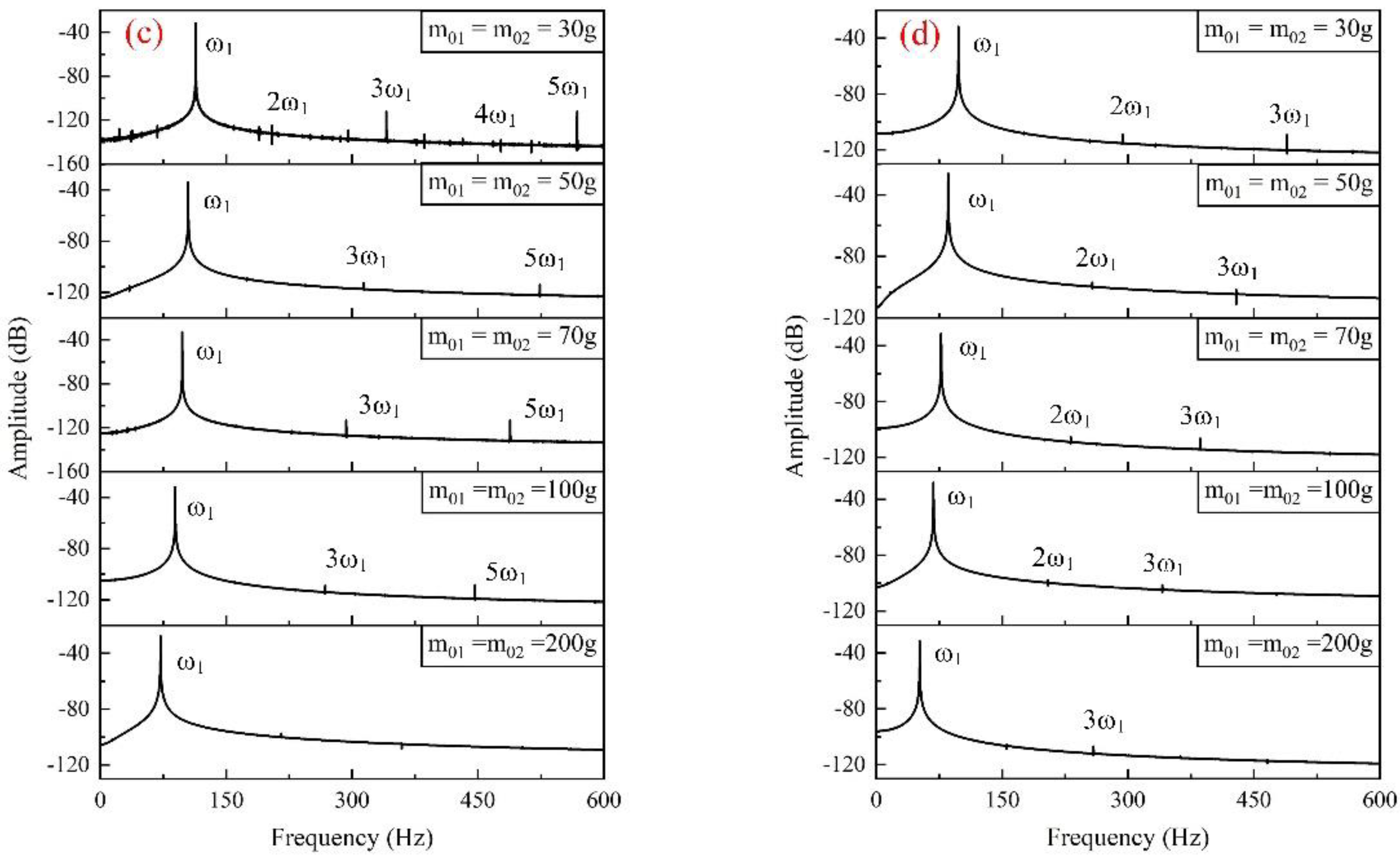
3.2. Symmetric Additional Mass

Based on the parameters provided in Section 3.1, the spectrogram of the system with additional mass was solved by defining the magnitudes and positions ${\xi }_1,{\xi }_2$ of the additional masses $m_{\mathrm{o}1},m_{\mathrm{o}2}$. To facilitate comparison, the effect of the symmetric additional mass on the system response was first studied based on actual conditions. Here, the magnitudes of the additional masses were 30 g, 50 g, 70 g, 100 g, and 200 g, and the positions of the additional masses were l/4, l/2, l×3/4, and l, respectively for cross-calculation. The spectrograms are shown in Figure 5, and the frequency and amplitude are shown in

Table 2. Frequencies and amplitudes.

Additional- Mass Position		Frequencies (Hz)						Amplitudes (dB)
		30 g	50 g	70 g	100 g	200 g		30 g	50 g	70 g	100 g	200 g
l/4	ω1	132.57	131.76	131.40	130.88	129.20	A1	−52.62	−27.75	−34.36	−34.77	−28.82
	2ω1	265.21	-	-	-	-	A2	−124.95	-	-	-	-
	3ω1	397.78	395.14	394.12	392.58	387.74	A3	−125.80	−104.52	−109.48	−107.90	−106.79
l/2	ω1	126.64	123.12	119.82	115.43	103.49	A1	−27.96	−34.73	−25.68	−24.84	−25.21
	2ω1	253.27	369.07	359.47	346.14	310.55	A2	−111.97	−111.41	−100.41	−98.39	−105.53
	3ω1	379.91	-	-	577.00	517.60	A3	−106.00	-	-	−98.99	−107.75
l×3/4	ω1	113.67	104.74	97.71	89.28	71.85	A1	−31.80	−34.12	−32.73	−31.81	−27.63
	2ω1	227.34	-	-	-	-	A2	−133.98	-	-	-	-
	3ω1	341.02	314.28	293.04	267.99	-	A3	−111.89	−112.65	−113.15	−108.63	-
	4ω1	454.69	-	-	-	-	A4	−139.24	-	-	-	-
	5ω1	568.36	523.75	488.38	446.56	-	A5	−112.00	−113.98	−113.08	−108.53	-
l	ω1	97.85	85.77	77.20	68.19	51.78	A1	−31.78	−26.24	−31.22	−28.02	−31.22
	2ω1	195.04	257.30	231.74	204.57	-	A2	−109.85	−97.07	−105.29	−97.89	-
	3ω1	293.55	428.91	386.13	341.02	258.91	A3	−109.07	−101.73	−106.45	−101.23	−106.76

.

Figure 5 shows vibration spectrograms of the coupling system with symmetric additional masses. From (a) to (d), the additional masses gradually move away from the base. In each (i), from top to bottom, the magnitudes of the additional masses gradually increase. At the left, the vertical coordinate indicates the signal-to-noise ratio, and the horizontal coordinate indicates the frequency.

Figure 5 shows that the change in the position of the same additional mass had a small effect on the natural frequency of the coupling system. However, such a change had a greater effect as the mass increased, and there was frequency doubling factor; the additional mass had a certain suppression effect on nonlinear frequency doubling and an obvious suppression effect on the low-frequency signal. Moreover, even the frequency doubling was suppressed and eliminated in priority. However, the natural frequency of the coupling system decreased with increasing additional mass. That resulted in a high-order frequency doubling in a low-frequency range and affected the measuring accuracy of the CMF at high frequency.

Table 2 shows that without reducing the natural frequency amplitude, the larger the mass, the better the suppression effect on the nonlinear frequency doubling amplitude. Taking l×3/4 as a boundary, on the side close to the base, the greater the distance from the base under the same mass or the larger the additional mass at the same position, the better the suppression effect on the nonlinear frequency doubling amplitude; if beyond l×3/4, the increase in mass had less effect on the suppression of nonlinear frequency doubling.

Figure 5 and Table 2 show that the greater the distance from the base, the better the suppression effect on nonlinear frequency doubling, but the more sensitive to the change in additional mass. At a small mass, low-frequency doubling was obviously suppressed, but high-frequency doubling was not suppressed. At this time, the entire system had a high natural frequency, so high-frequency doubling had a small effect on the measuring accuracy in a low-frequency range. However, the measuring accuracy decreased in a high-frequency range; at a larger mass, the low-frequency doubling was basically eliminated. However, with the decrease in the overall natural frequency of the system, the high-frequency doubling appeared prematurely in a low-frequency range. In that case, the CMF working frequency range was determined by the high-frequency range. Therefore, there were two types of nonlinear frequency doubling suppressions, namely nonlinear low-frequency doubling suppression and nonlinear high-frequency doubling suppression. By rationally designing the additional masses and relative positions, the working performance of the CMF within a certain frequency range can be improved.

3.3. Asymmetric Additional Mass

In Equation (20), the additional mass of two beams on the base and its position are independent variables. Accordingly, the additional mass on only one beam can be studied, and its effect on the coupling system can be observed. In the CMF manufacturing process, some asymmetries are caused by comprehensive errors, such as mold inaccuracy and machine tool machining errors. Those asymmetries occur mainly in the measuring tube itself and in dual measuring tubes, which in the latter include mainly mass asymmetry. If the CMF has been used for a long time, the measuring tube and the pipeline become corroded or worn, which also contributes to the mass asymmetry of dual measuring tubes. Therefore, research on asymmetric additional mass can facilitate actual error analysis and provide a basis for the nondestructive testing of CMF measuring tubes.

It can be seen from Equation (20) that the same results are obtained if the magnitude and position of an additional mass are equally changed at any of the magnitudes, which is verified by the calculation results, and only beam 1 is discussed here, given that $m_{\mathrm{o}2}=0; {\xi }_2=0$. Because the masses of double beams are different, two first-order frequencies definitely exist, whereas the CMF is a closed-loop system and outputs only one frequency. Here, for the convenience of discussion, the external force is ignored; i.e., double beams freely vibrate, and the rest of the parameters are kept the same as they are in Section 3.1. The results are summarised in Figure 6.

Figure 6 shows the spectrograms at four positions, 𝑙/4, 𝑙/2, 𝑙×3/4, and 𝑙, when additional mass is 30 g (a to d), 70 g (e to h) and 200 g (i to l). It can be seen from left to right in each row that, as the additional mass on a single beam is moved away from the base, the difference in the first-order natural frequency of the two separate beams gradually increased. In other words, the additional mass had a greater effect on the working frequency of the system. The additional mass had some suppression effect on the high-order frequency only when it was away from the base, but errors in low-order frequency were introduced. Note that, as shown in Figure 6g,h,k,l, the first two orders of frequency of the system; i.e., the first-order natural frequency of two beams, produced the beat frequency phenomenon. That phenomenon was related to the magnitude of the additional mass, but the asymmetric additional mass became one of the factors leading to nonlinear frequency doubling for coupled vibration. Also, as shown in Figure 6h,k,l, with the increase in additional mass, the high-order frequency of the system (such as Ω₃ and Ω₄) was a multiple of the natural frequency of the beam without additional mass, which demonstrates again that the frequency is transferred between beams through the base and further confirms the Huygens’ theory.

In conclusion, the asymmetric additional mass hindered the suppression of frequency doubling signals, but more burrs were found in the spectrum curve. However, the asymmetric additional mass was analyzed to determine the health of the CMF tubes. Further analysis with reference to Figure 6 provides a basis for the calibration of instruments in the actual industrial field.

4. Experiment and Analysis

Figure 7 shows the hardware configuration of the experimental platform, which included a dual U-tube CMF, an acceleration sensor distributed on the flowmeter, a signal acquisition system, and a computer. The flowmeter was horizontally suspended on the beam by a steel rope, and four accelerometers were rigidly connected to the bottoms of four beams of the flowmeter measuring tube. One accelerometer was rigidly connected to the base centre. In Figure 7, the four points a, b, c, and d indicate the positions of the additional masses, which corresponded to l/2, l×3/4, l and actuation position(Aq), respectively for numerical analysis and were the exciting point of the CMF. The additional masses were made of mass blocks with a unit of 1 g and were pasted at the designated positions with 3M double-sided adhesive, with the direction in line with the motion equation. The signal acquisition system contained seven channels. Self-developed data acquisition cards were used. The signal output by the accelerometer is represented by 1–4 and 7, and 5 and 6 were the output signals of the detection point of the CMF closed-loop system, marked as 1 to 7 in Figure 7. In the experiment, the data acquisition and storage program was written in the graphical programming language LabVIEW. The geometric parameters of the flowmeter measuring tube and the sensitivity of the accelerometer are shown in Figure 8 and

Table 3. Geometric parameters of measuring tube (mm).

B	R1	R2	H1	H2	H3	H4	D (Tube Wall Thickness)
260	60	54	240	180	23	48	1

and

Table 4. Sensitivity of accelerometer (mV/ms⁻²).

No.	Sensitivity
1	9.962
2	10.333
3	9.892
4	10.198
7	9.982

.

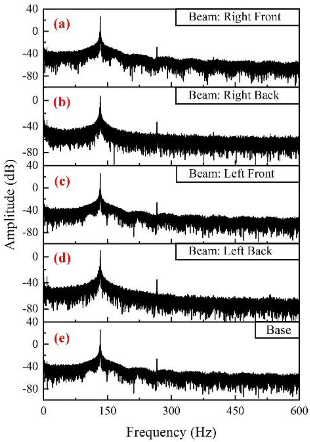
4.1. CMF without Additional Mass

Figure 9 shows a group of response spectrograms of the CMF double-beam coupled vibration model without additional mass, including vibration spectrograms of the signals from channels 1, 6, and 7. The resonant frequency and amplitude differences are shown in

Table 5. Resonance frequency (Hz) and amplitude difference (dB).

	ω1	2ω1	3ω1	A(ω1) − A(2ω1) (dB)	A(2ω1) − A(3ω1) (dB)
Beam	133.22	266.45	399.67	45.72	17.57
Detection position	133.22	266.45	399.67	45.72	17.57
Base	133.22	266.45	-	42.89	-

.

Figure 9 and Table 5 show that the vibration spectra output at the detection point of the CMF closed-loop system and at the pipe bottom were basically identical without additional mass. The same phenomenon was observed among the subsequent experimental data with symmetric additional mass. Note that the base of the coupling system experienced obvious frequency doubling vibration, which indicated that the base had negligible effects on the frequency doubling signals. Also, the vibration of double beams was coupled by the base, which also proves the necessity and correctness of establishing the Lagrange equation, including the base, in tracing nonlinear frequency doubling signals.

4.2. CMF with Symmetric Additional Mass

In accordance with the numerical model in Section 2, the dual U tube in the coupling system had to be simplified into double beams, in which case the symmetric additional mass specifically meant that the four beams with the same distance from the base had the same additional mass. In accordance with the conclusion given in Section 4.1, the output signal from the detection point of the CMF closed-loop system (channel 6) was used uniformly to observe the vibration of the coupling system with symmetric additional mass. The results of the spectrogram are shown in Figure 10, and the frequencies and amplitudes are given in

Table 6. Frequencies and amplitudes.

Frequencies (Hz)
Channel 1	Additional- mass position	1 g				3 g				5 g
		ω1	2ω1	3ω1	4ω1	ω1	2ω1	3ω1	4ω1	ω1	2ω1	3ω1	4ω1
	l/2	133.29	266.57	399.55	-	133.19	266.42	399.61	-	133.13	266.32	399.55	-
	l×3/4	133.10	266.16	399.26	-	132.81	265.66	398.47	531.32	132.56	265.15	397.72	-
	l	132.85	265.69	398.54	-	132.15	264.33	396.48	-	131.46	262.94	394.43	525.89
	Ap	132.91	265.85	-	-	132.34	264.49	396.80	-	131.65	263.32	395.00	-
Channel 2		1 g				3 g				5 g
		ω1	2ω1	3ω1	4ω1	ω1	2ω1	3ω1	4ω1	ω1	2ω1	3ω1	4ω1
	l/2	133.26	266.57	-	-	133.19	266.39	399.61	532.80	133.16	266.32	399.48	532.64
	l×3/4	132.94	265.79	-	-	132.81	265.66	-	-	132.59	265.19	397.75	530.34
	l	132.88	265.69	-	531.38	132.15	264.30	-	528.60	131.49	262.98	394.40	525.89
	Ap	132.91	265.82	-	-	132.31	264.68	396.80	529.14	131.71	263.32	395.03	526.68
Channel 7		1 g				3 g				5 g
		ω1	2ω1	3ω1	4ω1	ω1	2ω1	3ω1	4ω1	ω1	2ω1	3ω1	4ω1
	l/2	133.29	266.57	-	-	133.19	266.42	-	-	133.16	266.35	-	-
	l×3/4	133.10	266.16	-	-	132.85	265.66	-	-	132.59	265.15	-	-
	l	132.85	265.69	-	-	132.15	264.30	396.45	528.63	131.46	262.94	-	525.92
	Ap	132.91	265.82	-	-	132.31	264.65	396.80	-	131.65	263.32	395.00	526.68
Amplitudes (dB)
Channel 1		1 g				3 g				5 g
		A1	A2	A3	A4	A1	A2	A3	A4	A1	A2	A3	A4
	l/2	21.90	−26.40	−44.22	-	22.67	−25.31	−41.60	-	18.94	−25.67	−46.66	-
	l×3/4	24.53	−25.41	−42.52	-	27.39	−24.61	−40.22	−48.34	29.20	−22.57	−42.42	-
	l	28.74	−24.95	−43.45	-	34.29	−27.18	−39.43	-	35.03	−19.88	−35.81	−37.03
	Ap	26.37	−28.26	-	-	30.94	−31.47	−37.08	-	33.73	−29.10	−33.03	-
Channel 2		1 g				3 g				5 g
		A1	A2	A3	A4	A1	A2	A3	A4	A1	A2	A3	A4
	l/2	10.23	−30.28	-	-	13.21	−29.87	−47.43	−45.67	11.30	−26.50	−46.98	−44.79
	l×3/4	3.68	−34.22	-	-	14.51	−27.19	-	-	24.94	−22.69	−41.70	−45.55
	l	13.84	−27.43	-	−45.44	30.40	−28.86	-	−47.29	33.84	−23.63	−36.96	−36.19
	Ap	6.40	−33.11	-	-	24.38	−32.80	−43.37	−46.86	29.24	−32.68	−40.62	−48.38
Channel 7		1 g				3 g				5 g
		A1	A2	A3	A4	A1	A2	A3	A4	A1	A2	A3	A4
	l/2	19.63	−25.35	-	-	20.74	−23.24	-	-	21.43	−22.46	-	-
	l×3/4	22.21	−22.90	-	-	26.24	−25.31	-	-	29.27	−19.68	-	-
	l	27.65	−22.70	-	-	33.81	−24.03	−43.12	−45.71	34.36	−15.20	-	−43.60
	Ap	25.73	−26.36	-	-	27.57	−30.70	−38.31	-	33.10	−27.46	−32.78	−48.11

.

The experimental results showed that the additional mass was much smaller than the mass of the measuring tube and had little effect on the frequency corresponding to each order of modal. However, the additional mass at different positions had an important effect on the frequency doubling signals, and the frequency doubling signals could be suppressed.

Same mass but different positions: the experimental results showed that, for a small mass, the greater the distance from the base, the better the suppression effect of the nonlinear frequency doubling phenomenon. However, the suppression of the nonlinear frequency doubling amplitude was affected: as the additional mass increased, the less the distance away from the base, the better the suppression effect of the nonlinear frequency doubling phenomenon and nonlinear frequency doubling amplitude.

Same position but different masses: at l/2, the greater the mass, the better the suppression effect of the nonlinear frequency doubling phenomenon and frequency doubling amplitude. Also, the less the random noise, the smoother the spectrogram: some impurity peaks gradually weakened or disappeared and had a good suppression effect on low-order frequency doubling. At l×3/4, the nonlinear suppression effect of different masses showed little difference. However, as the mass increased, the high-frequency doubling was markedly suppressed; relatively, at l, the smaller the mass, the better the suppression effect.

Because the exciting unit of the CMF was arranged in the centre of the U tube, considering the effect of additional mass in the exciting unit, the experimental results showed that the additional mass had less effect on the nonlinear frequency doubling, but the random noise could be reduced by additional mass.

Through the experiment on symmetric additional mass, the conclusion was in line with the numerical analysis. From the perspective of actual operation, to suppress the nonlinear low-frequency doubling of the coupling system, a small mass far from the base or a large mass close to the base was selected as a priority. To suppress the nonlinear high frequency, a symmetric additional mass was arranged at l×3/4 as a priority, but the magnitude of the mass needed to be obtained by more dynamic balance experiments.

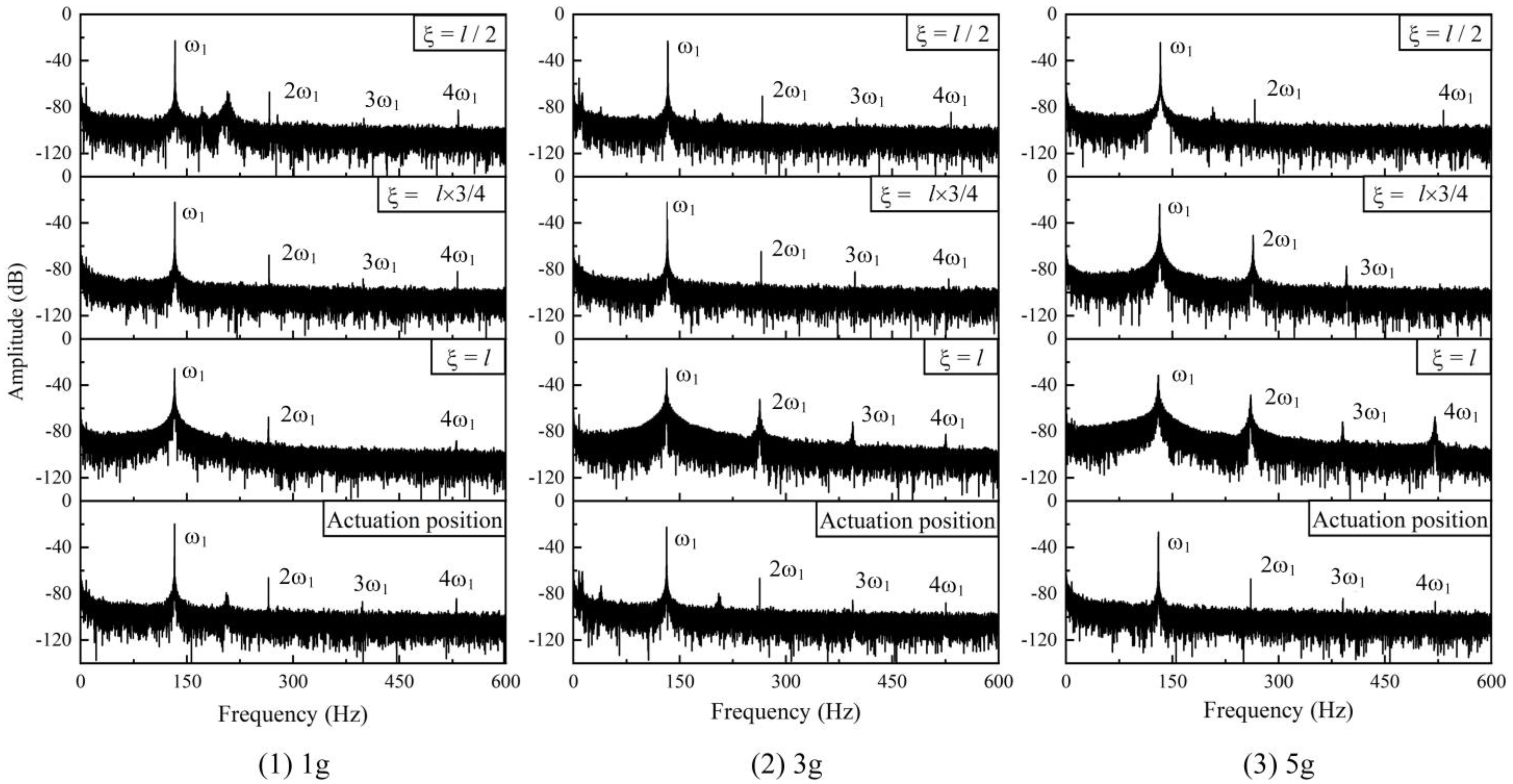
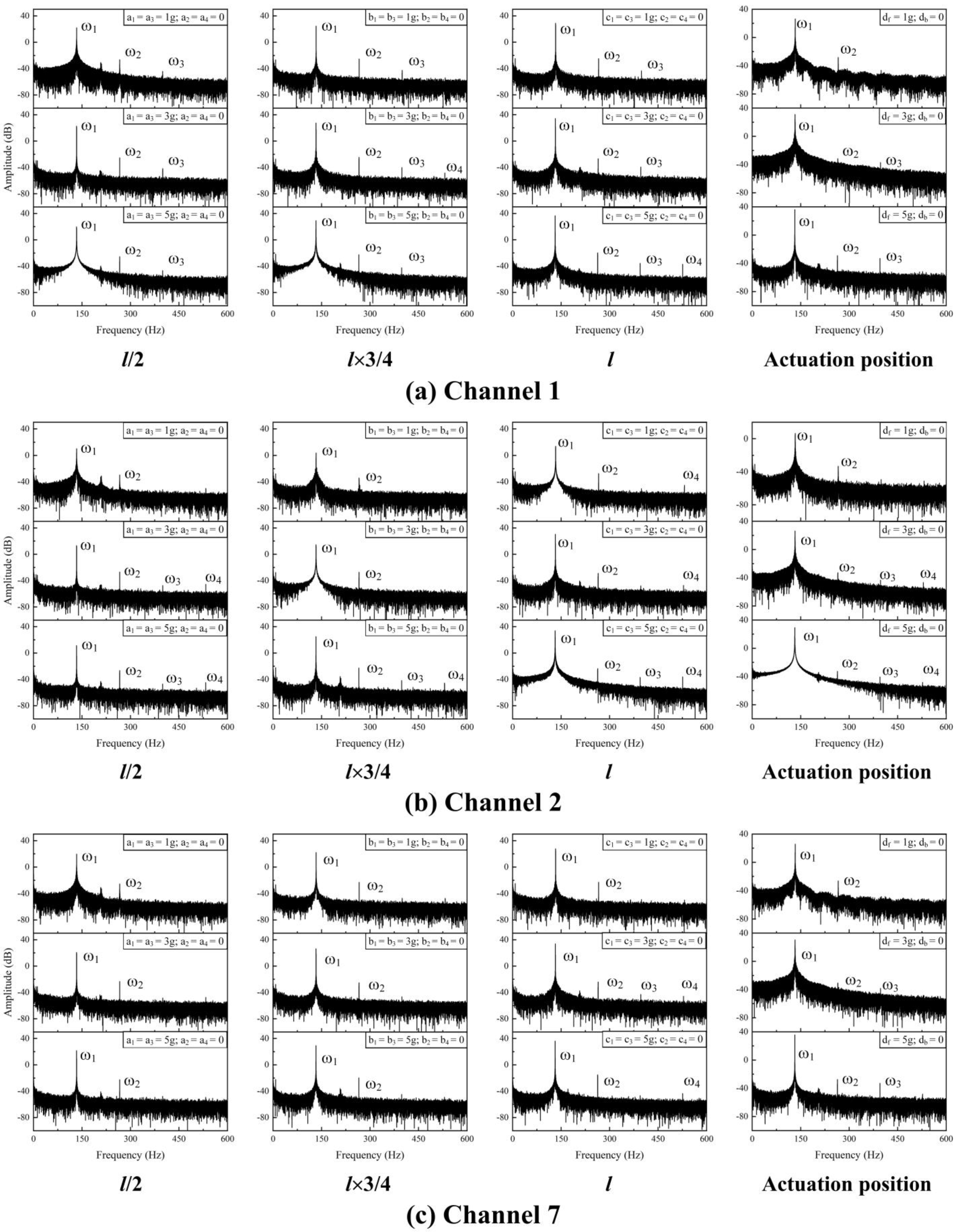
4.3. CMF with Asymmetric Additional Mass

With the help of the experimental platform, the effect of the asymmetric additional mass on the frequency doubling phenomenon was studied. For the dual-tube CMF used in the experiments, four beams were connected to the base. The asymmetric additional mass can be divided into three types by placement positions: symmetric additional masses (pipe 1 and 3, 2 and 4) were placed only on double beams in the same U tube; symmetric additional masses (pipe 1 and 2, 3 and 4) were placed on the same side of different U tubes, and an additional mass was placed on a beam. In the latter two cases, the CMF may produce a second-order-like motion in the first order, or the CMF was under gradual oscillation. Only the first asymmetric case is discussed here.

Figure 11 shows the vibration spectrograms of the beams and base only with additional mass a₁ = 1 g. From top to bottom, the vibrations at the bottoms of four beams and the base are given, where (a) and (c), (b) and (d) indicate the two beams in the same tube. It can be seen that double beams in the same U tube experience the same vibration, and the vibration of a single beam cannot be obtained at the detection point of the CMF itself. To simplify the picture information, only the vibration information of channels 1, 2, and 7 must be summarised. The vibration spectrograms of the three masses at four positions are shown in Figure 12, where (a), (b), and (c) correspond to the three channels 1, 2, and 7 respectively. Each channel comprises four pictures, corresponding to four positions l/2, l×3/4, l, and the actuation position(Aq), each of which contains three additional masses, namely 1, 3, and 5. Their corresponding frequency and amplitude are given in

Table 7. Frequencies and amplitudes.

Frequencies (Hz)
Channel 1	Additional- mass position	1 g				3 g				5 g
		ω1	ω2	ω3	ω4	ω1	ω2	ω3	ω4	ω1	ω2	ω3	ω4
	l/2	133.29	266.57	399.55	-	133.19	266.42	399.61	-	133.13	266.32	399.55	-
	l×3/4	133.10	266.16	399.26	-	132.81	265.66	398.47	531.32	132.56	265.15	397.72	-
	l	132.85	265.69	398.54	-	132.15	264.33	396.48	-	131.46	262.94	394.43	525.89
	Ap	132.91	265.85	-	-	132.34	264.49	396.80	-	131.65	263.32	395.00	-
Channel 2		1 g				3 g				5 g
		ω1	ω2	ω3	ω4	ω1	ω2	ω3	ω4	ω1	ω2	ω3	ω4
	l/2	133.26	266.57	-	-	133.19	266.39	399.61	532.80	133.16	266.32	399.48	532.64
	l×3/4	132.94	265.79	-	-	132.81	265.66	-	-	132.59	265.19	397.75	530.34
	l	132.88	265.69	-	531.38	132.15	264.30	-	528.60	131.49	262.98	394.40	525.89
	Ap	132.91	265.82	-	-	132.31	264.68	396.80	529.14	131.71	263.32	395.03	526.68
Channel 7		1 g				3 g				5 g
		ω1	ω2	ω3	ω4	ω1	ω2	ω3	ω4	ω1	ω2	ω3	ω4
	l/2	133.29	266.57	-	-	133.19	266.42	-	-	133.16	266.35	-	-
	l×3/4	133.10	266.16	-	-	132.85	265.66	-	-	132.59	265.15	-	-
	l	132.85	265.69	-	-	132.15	264.30	396.45	528.63	131.46	262.94	-	525.92
	Ap	132.91	265.82	-	-	132.31	264.65	396.80	-	131.65	263.32	395.00	526.68
Amplitudes(dB)
Channel 1		1 g				3 g				5 g
		A1	A2	A3	A4	A1	A2	A3	A4	A1	A2	A3	A4
	l/2	21.90	−26.40	−44.22	-	22.67	−25.31	−41.60	-	18.94	−25.67	−46.66	-
	l×3/4	24.53	−25.41	−42.52	-	27.39	−24.61	−40.22	−48.34	29.20	−22.57	−42.42	-
	l	28.74	−24.95	−43.45	-	34.29	−27.18	−39.43	-	35.03	−19.88	−35.81	−37.03
	Ap	26.37	−28.26	-	-	30.94	−31.47	−37.08	-	33.73	−29.10	−33.03	-
Channel 2		1 g				3 g				5 g
		A1	A2	A3	A4	A1	A2	A3	A4	A1	A2	A3	A4
	l/2	10.23	−30.28	-	-	13.21	−29.87	−47.43	−45.67	11.30	−26.50	−46.98	−44.79
	l×3/4	3.68	−34.22	-	-	14.51	−27.19	-	-	24.94	−22.69	−41.70	−45.55
	l	13.84	−27.43	-	−45.44	30.40	−28.86	-	−47.29	33.84	−23.63	−36.96	−36.19
	Ap	6.40	−33.11	-	-	24.38	−32.80	−43.37	−46.86	29.24	−32.68	−40.62	−48.38
Channel 7		1 g				3 g				5 g
		A1	A2	A3	A4	A1	A2	A3	A4	A1	A2	A3	A4
	l/2	19.63	−25.35	-	-	20.74	−23.24	-	-	21.43	−22.46	-	-
	l×3/4	22.21	−22.90	-	-	26.24	−25.31	-	-	29.27	−19.68	-	-
	l	27.65	−22.70	-	-	33.81	−24.03	−43.12	−45.71	34.36	−15.20	-	−43.60
	Ap	25.73	−26.36	-	-	27.57	−30.70	−38.31	-	33.10	−27.46	−32.78	−48.11

.

Figure 12 shows that the suppression effect of the asymmetric additional mass on the nonlinear frequency doubling phenomenon was basically the same as that of the symmetric additional mass. The larger the additional mass and the closer to the base, the better the suppression effect on the nonlinear frequency doubling phenomenon. However, in conjunction with Table 7, for the asymmetric additional mass on the beams, the larger the additional mass, and the farther from the base, the better the suppression effect on the frequency doubling amplitude. The overall amplitude of the beams increases under additional mass, however, so the high-order frequency doubling amplitude gradually became prominent. The overall nonlinear suppression effect of the asymmetric additional mass on the beams without additional mass was the best at the greatest distance and the maximum mass. The frequency spectrum of channel 7 showed that a nonlinear additional mass had little effect on nonlinear frequency doubling; only when the additional mass was at the maximum did it have an obvious suppression effect on nonlinear frequency doubling.

In conclusion, the asymmetric additional mass hindered the suppression of the frequency doubling signal, and the nonlinear frequency doubling phenomenon and the nonlinear frequency doubling amplitude suppression cannot be suppressed simultaneously. However, it was found that when the asymmetric additional mass was small, there was a positive suppression effect on the coupling system. However, when the additional mass was pipeline appendages, pipeline wear, machining defects, etc., as the mass increased, the frequency doubling phenomenon tended to result in a spectrogram for symmetric additional mass, which would affect the further suppression of the nonlinear frequency doubling signal, leading to judgement errors.

5. Conclusions and Prospects

In this study, based on previous theoretical derivations and actual industrial demand, the effect of symmetric and asymmetric additional masses on the nonlinear frequency doubling of a coupling system was studied by introducing additional mass into the theoretical model. The effect of additional mass was further verified and explored through experiments. The final experimental and numerical analysis results were basically consistent; that is, the nonlinear frequency doubling phenomenon can be addressed based on industrial requirements from the two perspectives of low-frequency suppression and high-frequency suppression. A CMF can be specifically designed in accordance with the requirements for the working environment and measuring accuracy: for a CMF with higher measuring accuracy requirements for low frequencies, mass can be added on the beams near or far from the base. For a CMF with higher measuring accuracy requirements for high frequencies, mass can be added at the far end of the beams, thus achieving high-frequency doubling suppression and improving the CMF performance.

When the asymmetric additional masses were small, there was a certain suppression effect. However, as the additional mass increased, the suppression effect gradually became a frequency doubling phenomenon. Because of the natural frequency doubling phenomenon of the CMF, asymmetric additional mass can be easily overlooked. This meant that in industrial work, an asymmetry of the measuring tube mass resulting from pipeline appendages, pipeline wear, processing defects, etc. is easily detected only with a small mass. As the mass increases, the effect can be easily confused with the frequency doubling phenomenon of the CMF.

In summary, the conclusions of this study have certain guiding significance for the suppression of the nonlinear frequency doubling phenomenon of flowmeters in actual industrial production and provide favourable technical support for CMF R&D. Because the numerical model and the actual CMF are still different, we will continue to improve the digital modelling, increase the difference in additional mass, and provide clearer guidance for developing CMFs and eliminating nonlinearity.

References

1. Zheng, D.; Wang, S.; Fan, S. Nonlinear Vibration Characteristics of Coriolis Mass Flowmeter. Chin. J. Aeronaut. 2009, 22, 198–205. [Google Scholar] [CrossRef] [Green Version]
2. Zheng, D.; Wang, S.; Liu, B.; Fan, S. Theoretical analysis and experimental study of Coriolis mass flow sensor sensitivity. J. Fluids Struct. 2016, 65, 295–312. [Google Scholar] [CrossRef]
3. Belhadj, A.; Cheesewright, R.; Clark, C. The simulation of coriolis meter response to pulsating flow using a general purpose F.E. code. J. Fluids Struct. 2000, 14, 613–634. [Google Scholar] [CrossRef]
4. Chen, S.-S. Dynamic Stability of Tube Conveying Fluid. J. Eng. Mech. Div. 1971, 97, 1469–1485. [Google Scholar] [CrossRef]
5. Enz, S.; Thomsen, J.J. Predicting phase shift effects for vibrating fluid-conveying pipes due to Coriolis forces and fluid pulsation. J. Sound Vib. 2011, 330, 5096–5113. [Google Scholar] [CrossRef]
6. Wang, T.; Baker, R. Manufacturing variation of the measuring tube in a Coriolis flowmeter. Comput. Control. Eng. J. 2003, 14, 38–39. [Google Scholar] [CrossRef]
7. Bobovnik, G.; Mole, N.; Kutin, J.; Štok, B.; Bajsić, I. Coupled finite-volume/finite-element modelling of the straight-tube Coriolis flowmeter. J. Fluids Struct. 2005, 20, 785–800. [Google Scholar] [CrossRef]
8. Bobovnik, G.; Kutin, J.; Mole, N.; Štok, B.; Bajsić, I. Numerical analysis of installation effects in Coriolis flowmeters: Single and twin tube configurations. Flow Meas. Instrum. 2015, 44, 71–78. [Google Scholar] [CrossRef]
9. Keita, N. Contribution to the understanding of the zero shift effects in Coriolis mass flowmeters. Flow Meas. Instrum. 1989, 1, 39–43. [Google Scholar] [CrossRef]
10. Thomsen, J.J.; Dahl, J. Phase shift effects for fluid conveying pipes on non-ideal supports. J. Sound Vib. 2010, 329, 3065–3081. [Google Scholar] [CrossRef]
11. Thomsen, J.J.; Dahl, J.; Fuglede, N.; Enz, S. Predicting phase shift of elastic waves in pipes due to fluid flow and imperfections. In Proceedings of the 16th International Congress on Sound and Vibration, ICSV16, Krakow, Poland, 5–9 July 2009; p. 8. [Google Scholar]
12. Hemp, J.; Kutin, J. Theory of errors in Coriolis flowmeter readings due to compressibility of the fluid being metered. Flow Meas. Instrum. 2006, 17, 359–369. [Google Scholar] [CrossRef]
13. Fuglede, N. Coriolis Flowmeter Accuracy and Precision; Technical University of Denmark: Lyngby, Denmark, 2009. [Google Scholar]
14. Gagliano, S.; Cairone, F.; Amenta, A.; Bucolo, M. A Real Time Feed Forward Control of Slug Flow in Microchannels. Energies 2019, 12, 2556. [Google Scholar] [CrossRef] [Green Version]
15. Gagliano, S.; Stella, G.; Bucolo, M. Real-Time Detection of Slug Velocity in Microchannels. Micromachines 2020, 11, 241. [Google Scholar] [CrossRef] [PubMed] [Green Version]
16. Senator, M. Synchronization of two coupled escapement-driven pendulum clocks. J. Sound Vib. 2006, 291, 566–603. [Google Scholar] [CrossRef]
17. Neda, Z.; Ravasz, E.; Brechet, Y.; Vicsek, T.; Barabasi, A. The sound of many hands clapping. Nat. Cell Biol. 2000, 403, 849–850. [Google Scholar] [CrossRef]
18. Néda, Z.; Ravasz, E.; Vicsek, T.; Brechet, Y.; Barabasi, A. Physics of the rhythmic applause. Phys. Rev. E 2000, 61, 6987–6992. [Google Scholar] [CrossRef] [Green Version]
19. Kapitaniak, M.; Czolczynski, K.; Perlikowski, P.; Stefanski, A.; Kapitaniak, T. Synchronization of clocks. Phys. Rep. 2012, 517, 1–69. [Google Scholar] [CrossRef] [Green Version]
20. Wu, Y.; Wang, N.; Li, L.; Xiao, J. Anti-phase synchronization of two coupled mechanical metronomes. CHAOS Interdiscip. J. Nonlinear Sci. 2012, 22, 23146. [Google Scholar] [CrossRef]
21. Xin, X.; Liu, Y. Analysis of synchronization phenomena of two metronomes on a cart using describing function approach. In Proceedings of the 2015 American Control Conference, Chicago, IL, USA, 1–3 July 2015; IEEE: Piscataway, NJ, USA, 2015; pp. 1345–1350. [Google Scholar]
22. Li, Z.X.; Hu, C.; Zheng, D.Z.; Fan, S.C. Synchronization Theory-Based Analysis of Coupled Vibrations of Dual-Tube Coriolis Mass Flowmeters. Sensors 2020, 20, 6340. [Google Scholar] [CrossRef] [PubMed]
23. Esu, O.E.; Wang, Y.; Chryssanthopoulos, M.K. Local vibration mode pairs for damage identification in axisymmetric tubular structures. J. Sound Vib. 2021, 494, 115845. [Google Scholar] [CrossRef]
24. G Krishnanunni, C.; N Rao, B. Indirect health monitoring of bridges using Tikhonov regularization scheme and signal averaging technique. Struct. Control Health Monit. 2021, 28, e2686. [Google Scholar]
Figure 1. Diagram of Huygens’ experimental device for pendulum synchronization.
Applsci 11 09916 g001
Figure 2. Structure diagram of a U-tube Coriolis mass flowmeter.
Applsci 11 09916 g002
Figure 3. Double-beam coupled vibration model with additional mass.
Applsci 11 09916 g003
Figure 4. Response spectrogram of double-beam coupled vibration model.
Applsci 11 09916 g004
Figure 5. Vibration spectrograms of coupling system with symmetric additional masses of different weight in different location. (a) Symmetric additional masses (top to bottom: 30 g, 50 g, 70 g, 100 g, and 200 g) in l/4. (b) Symmetric additional masses (top to bottom: 30 g, 50 g, 70 g, 100 g, and 200 g) in l/2. (c) Symmetric additional masses (top to bottom: 30 g, 50 g, 70 g, 100 g, and 200 g) in l×3/4. (d) Symmetric additional masses (top to bottom: 30 g, 50 g, 70 g, 100 g, and 200 g) in l.
Applsci 11 09916 g005aApplsci 11 09916 g005b
Figure 6. Response spectrogram of coupled vibration model of double beams with asymmetric additional mass. (ad) Asymmetric additional masses in beam 1 (m01 = 30 g) with different locations (left to right: 𝑙/4, 𝑙/2, 𝑙×3/4, and 𝑙). (eh) Asymmetric additional masses in beam 1 (m01 = 70 g) with different locations (left to right: 𝑙/4, 𝑙/2, 𝑙×3/4, and 𝑙). (il) Asymmetric additional masses in beam 1 (m01 = 200 g) with different location (left to right: 𝑙/4, 𝑙/2, 𝑙×3/4, and 𝑙).
Applsci 11 09916 g006
Figure 7. Hardware configuration of experimental platform.
Applsci 11 09916 g007
Figure 8. Schematic diagram of geometric modelling of dual U tube with fixed electrode distance.
Applsci 11 09916 g008
Figure 9. Response spectrogram of CMF double-beam coupled vibration model without additional mass. (a) Channel 1. (b) Channel 6. (c) Channel 7.
Applsci 11 09916 g009
Figure 10. Vibration spectrogram of coupling system with symmetric additional mass.
Applsci 11 09916 g010
Figure 11. Vibration frequency diagram of beams and base only with additional mass a1 = 1 g.
Applsci 11 09916 g011
Figure 12. Vibration spectrum diagram of asymmetric additional mass.
Applsci 11 09916 g012