Benchmarking Deep Learning Methods for Aspect Level Sentiment Classification

Abstract

With the advancements in processing units and easy availability of cloud-based GPU servers, many deep learning-based methods have been proposed for Aspect Level Sentiment Classification (ALSC) literature. With this increase in the number of deep learning methods proposed in ALSC literature, it has become difficult to ascertain the performance difference of one method over the other. To this end, our study provides a statistical comparison of the performance of 35 recent deep learning methods with respect to three performance metrics-Accuracy, Macro F1 score, and Time. The methods are evaluated for eight benchmark datasets. In this study, the statistical comparison is based on Friedman, Nemenyi, and Wilcoxon tests. As per the results of statistical tests, the top-ranking methods could not significantly outperform several other methods in terms of Accuracy and Macro F1 score and performed poorly on-time metric. However, the time taken by any method is crucial to analyze the overall performance. Thus, this study aids the selection of the Deep Learning method, which maximizes the accuracy and Macro F1 score and takes minimal time. Our study also establishes a framework for validating the performance of new and alternate methods in ALSC that can be helpful for researchers and practitioners working in this area.

1. Introduction

The widespread use of e-commerce and social media in the 21st century has led to the generation of massive unstructured data which is publicly accessible. This unstructured data primarily consists of user reviews regarding products and services as well as opinions and emotions on social and political issues. The unstructured data may be in the form of text, images, audio, video, and emoticons. The automated analysis of this unstructured data is of enormous importance to successful business organizations and governments. This has led to the emergence of Affective Computing and Sentiment Analysis as a specific discipline within Artificial Intelligence [1].

Analysis of sentiments from the textual opinions can be carried out at various levels: document level, sentence level, and aspect level [2]. In contrast to coarse-grained and overall sentiment analysis, Aspect Based Sentiment Analysis (ABSA) analyzes the sentiments of specific attributes or aspects of a product or service. The task of ABSA is further divided into three main sub-tasks mainly, Aspect Extraction (AE), Aspect Category Detection (ACD), and Aspect Level Sentiment Classification (ALSC). In ABSA, first, an aspect of a product or service is extracted from the text, and this task is known as Aspect Extraction (AE). Further, extracted aspects are mapped to a specific category, and this task is known as Aspect Category Detection (ACD). Finally, the task of determining the sentiment polarity of an aspect is performed. This task is named as Aspect Level Sentiment Classification (ALSC).

Traditionally, ABSA is performed either with the help of statistical methods or using machine learning with efficient feature engineering techniques [2,3,4]. Feature engineering is a time-consuming task and performing ABSA using traditional methods requires large domain-specific datasets and expert knowledge [5,6]. As an alternative, Deep Learning (DL) based methods are competent to learn continuous features from data without any feature engineering. In addition, deep learning methods are also efficient in capturing the relatedness between context and target. The easy availability of GPU and cloud-based computational resources has made it feasible to train deep neural networks efficiently at a low cost. Thus, in recent years, many deep learning methods, mainly Convolution Neural Networks (CNN), Memory Networks, Recurrent Neural Networks (RNN), and their multiple variants, have been proposed for ALSC [7]. The difference between Traditional and Deep learning-based ALSC can be well understood with the help of Figure 1.

With a surge in usage of deep learning methods to perform the ALSC task [8], it is imperative to ascertain whether the newly proposed methods improve over the previous models in a statistically significant way. Most of the existing deep learning methods are ignored by the researchers for comparison while proposing their new method. In addition, none of the comparative studies [7,8] perform a statistical comparison of the newly proposed model with existing deep learning-based models for ALSC. Furthermore, existing studies do not compare the newly proposed deep learning methods with existing methods in terms of training time.

The significant contribution of our study is that it provides a statistical comparison of state-of-the-art deep learning methods available in ALSC literature up to 2021 that include RNNs, Memory Networks, CNNs, the latest Hybrid Networks, and BERT-based methods. The statistical comparison is carried for three evaluation metrics that are Accuracy, Macro F1 score, and Time. To the best of our knowledge, this is the first study in which training time is considered for evaluating the performance of deep learning methods in ALSC.

The statistical comparison performed in our paper looks out for statistical evidence for the enhanced performance of recently proposed advanced deep learning methods in ALSC. Friedman test [9] and post hoc tests viz. Nemenyi test [10] and Wilcoxon test [9,11] are applied to experimental results of various deep learning methods across eight datasets of different domains.

This study addresses the following research question (RQ):

Is there any statistically significant difference in the performance of various deep learning methods proposed in ALSC literature from 2016 to 2021 in terms of Accuracy, Macro F1 score, and Time?

The rest of this paper is organized as: Section 2 introduces the ABSA, its sub-tasks, and ALSC. Section 3 discusses the technical details of deep learning methods studied in this work. The information related to datasets and experimental settings, along with statistical test details, is explained in Section 4. Section 5 provides an analysis of results and answers the research question addressed in this study. Finally, the conclusion and future work are presented in Section 6.

2. Overview of ABSA

This section is divided into two subparts. Section 2.1 discusses in detail ABSA, its various subtasks, and Section 2.2 describes the ALSC task in detail.

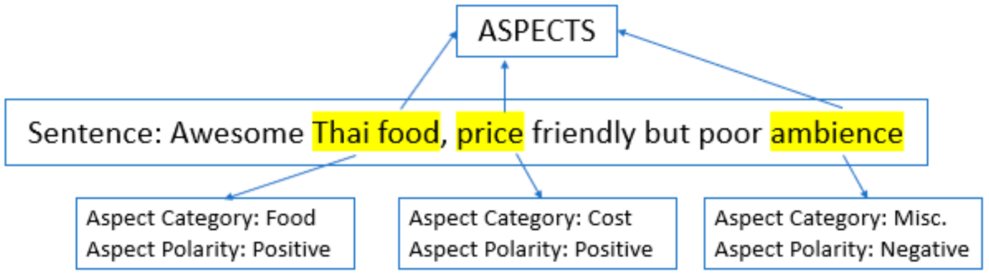
2.1. Aspect Based Sentiment Analysis

The fine-grained analysis of sentiments for extracting various aspects and detecting the polarities of the extracted aspects [12] is referred to as Aspect Based Sentiment Analysis (ABSA). ABSA can be further divided into mainly three main sub-tasks [13]: (a) Aspect Extraction (AE) or Opinion Target Extraction (OTE), (b) Detecting the Aspect Category, and (c) Determining the sentiment polarity of aspect. Many studies have been carried in recent years, dealing with one, two, or all three subtasks of ABSA.

In this case, e.g., consider the sentence in Figure 2, “Awesome Thai food, price friendly but poor ambience”, Thai food, price, and ambience are aspects where ‘Thai food’ belongs to category {food}, ‘price’ belongs to category {cost} and ‘ambience’ belongs to category {miscellaneous}. Further, the sentiment polarity of ‘Thai food’, ‘price’, and ‘ambience’ is positive, positive, and negative, respectively.

Since this study deals with the statistical comparison of various deep learning methods proposed in ALSC literature, thus in the subsequent section, the ALSC task is explained in detail.

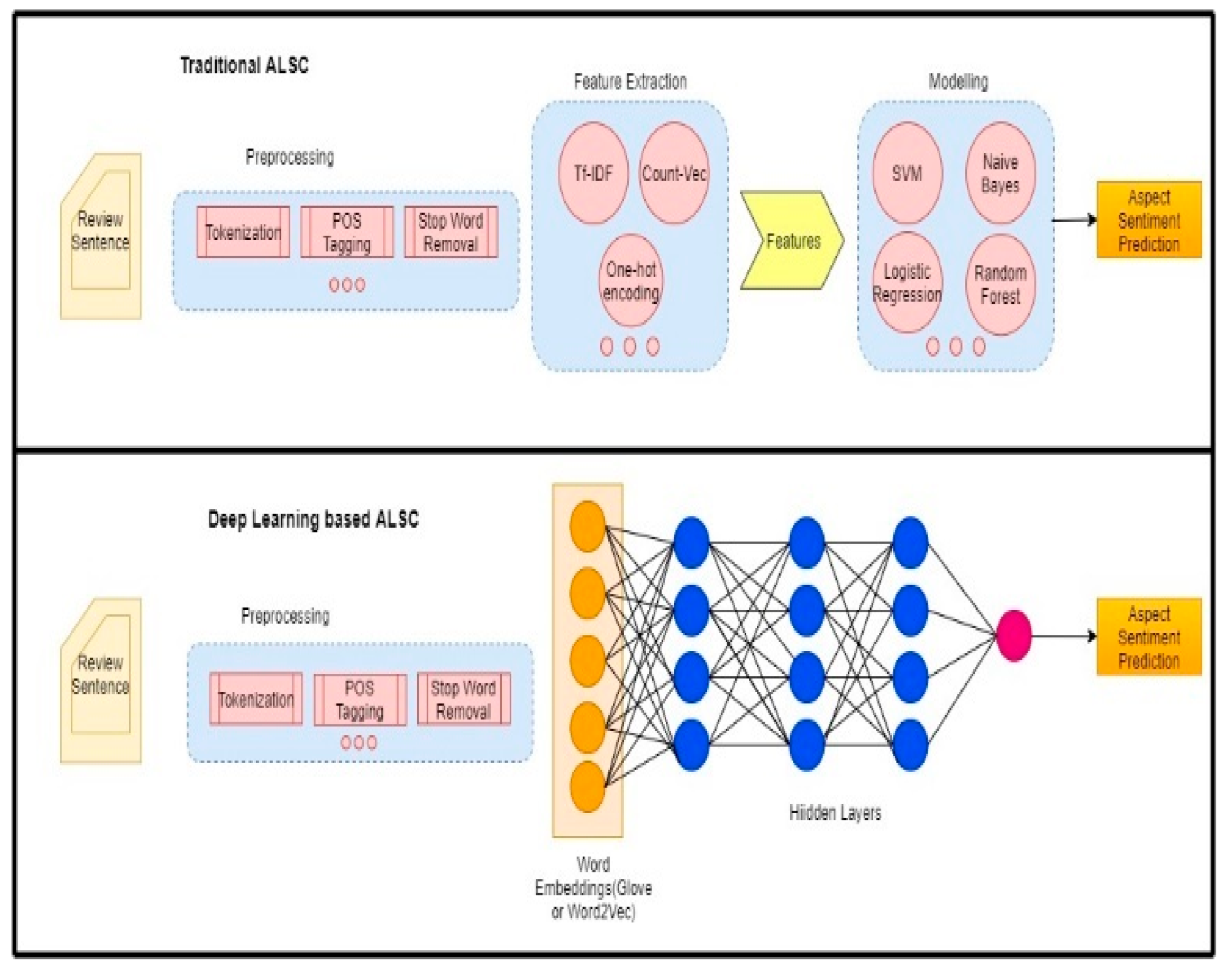
2.2. Aspect Level Sentiment Classification (ALSC)

The aspects discussed in the ALSC task can be either implicit or explicit aspects. An implicit aspect expresses an opinion about some feature of a product without explicitly using a target term for that feature. In contrast to this, the explicit aspect expresses an opinion about some feature of a product by explicitly mentioning the target term. Thus, ALSC is often interchangeably called Target dependent sentiment classification as well. Essentially, the terms ‘aspect’ and ‘target’ are used interchangeably by many researchers. For a better understanding of these two terms, consider the sentence in Figure 3: “The Mobile Phone is quite bulky, but the camera is great”. Here we have two types of aspects of the mobile phone handset, explicit and implicit [2]. The first phrase, “The Mobile phone is bulky” talks about the implicit aspect ‘weight’ while the second phrase, “the camera is great”, describes the explicit aspect “camera”. So, the camera is an explicit aspect term as well as the target word.

In short, we can use target and aspect interchangeably when we are dealing with explicit aspect terms. Finally, the task of ALSC is to map these aspects with suitable sentiment polarity. As per Figure 3, the polarity of explicit aspect “Camera” is positive while the polarity of implicit aspect “bulky” refers to the feature of mobile phone, and the polarity is negative. Most of the research in ALSC is been carried out for explicit aspects and thus the sentiment classification of implicit aspect is out of the scope of this study.

3. Deep Learning Methods for Aspect Level Sentiment Classification

This study aims to provide a statistical comparison of various deep learning methods proposed in ALSC literature. Section 3.1 discusses the recent work in deep learning-based ALSC. Afterward, Section 3.2 discusses the data modelling procedure for deep learning-based ALSC.

3.1. Recent Trends in Aspect Level Sentiment Classification

ALSC can be performed using three main approaches: unsupervised, semi- supervised, and supervised. The unsupervised and semi supervised techniques mainly follow corpus based and lexicon-based approaches [14]. The corpus-based approach utilizes the domain specific large corpora for generating relevant information, which requires substantial manual effort, extensive training, and big data. The lexicon-based approach (also known as the knowledge-based approach) works with external sentiment knowledge bases known as lexicons. Such techniques are entirely dependent on the quality of the knowledge base and often suffers the problem of the limited word (or out of vocabulary) [15].

The supervised ALSC can be carried using conventional or deep learning methods. The conventional (also known as machine learning-based) techniques require extensive feature engineering, while deep learning methods can work efficiently without feature engineering. Thus, recently ALSC researchers are inclined more towards deep learning -based approaches. Deep Learning is a learning paradigm that utilizes artificial neural networks for the efficient learning process and has recently gained importance in many tasks related to NLP such as text summarization [16], machine translation [17], question answering [18], etc. Deep learning methods utilized for sentiment analysis have also proven to perform better than traditional methods. The ensemble of deep learning methods with symbolic models has also been leveraged to create a sentiment lexicon. Senticnet5 [19] and Senticnet6 [20] are the lexicons generated by combining symbolic and sub-symbolic paradigms of AI. The symbolic paradigms refer to the use of logic and semantic network, and sub-symbolic refers to the usage of deep learning methods to encode the meaning of words in the lexicon.

In ALSC, the classification is reliant on the semantic structure of sentences, thus researchers have widely utilized LSTM in the field of ALSC. LSTM with the capability of handling non-linear data has proven to be successful for this task. Tang et al. [21] used LSTM for the ALSC task for the first time. The authors also proposed two variants of LSTM called TD-LSTM and TC-LSTM. Later, Wang et al. [22] leveraged the idea of combining aspect embedding with LSTM. The authors also proposed the attention-based variant of LSTM known as ATAE-LSTM.

The integration of attention mechanisms in deep learning methods was initially proposed for computer vision tasks [23]. It has also been successfully applied on many NLP tasks [24,25]. Attention-based methods have the capability of capturing the significance of the context words. This feature makes attention-based deep learning methods more promising for ALSC [22,26,27,28].

Along with attention, memory networks have also been utilized for ALSC. Tang et al. [29] proposed a deep memory network by using a pre-trained word vector as memory. The authors leveraged the attention mechanism for updating memory. Chen et al. [30] proposed the Recurrent Attention Memory (RAM) method, which exploits attention mechanisms and uses hidden states generated by LSTM as memory.

Simple attention networks can generate noisy features as well. This problem can be resolved using Capsule networks [31,32]. The capsule network can dynamically route the spatial features from the lower layer to the upper layers. The hidden vectors generated from the lower layer are considered as one capsule, and the upper layer features are considered as another capsule.

Another limitation of a simple attention network is the incapability to handle long-range dependencies. The syntactical structure of a sentence plays a crucial role in resolving the issue of long-range dependencies. However, most deep learning-based methods have not leveraged the syntactical structure of the sentence. There are limited hybrid methods that have incorporated syntactical knowledge along with deep neural networks using Graph Convolutional networks (GCN) [33,34,35].

Another way of handling the syntactical information is with the usage of Graph Attention Network (GAT). Wang et al. [36] and Bai et al. [37] have leveraged Graph Attention networks for ALSC task. The GAT method proposed by Bai et al. [37] uses typed dependencies (i.e., dependency label or relation) for enhanced performance. The authors also utilized BERT (Bidirectional Encoder Representations from Transformers) [38] model to generate contextual embeddings. BERT is a pre-trained language model that has gained popularity in many NLP tasks, including ALSC. There are few attempts in literature exploring BERT for ALSC. The incorporation of BERT with the deep learning methods has shown promising results. Jiang et al. [31] leveraged BERT in embedding layer and encoding layer to generate contextual embeddings. Song et al. [39] utilized BERT embeddings as input to their proposed deep neural network. Yang et al. [40] used a pre-trained BERT model directly for prediction.

Figure 4 summarizes the 35 deep learning methods statistically tested for significant performance in this study across multiple datasets of different domains. For a fair comparison, the methods based on domain-specific corpus or domain-specific embeddings are not dealt with in this study.

3.2. Data Modelling Procedure for Deep Learning-Based ALSC

In ALSC, it is desired to detect the polarity of aspects contained in a sentence. A sentence with aspects is transformed into machine-readable vector form as an input to a deep learning network. This input to the network varies according to the architecture of the deep learning method.

Table 1. Deep learning methods with their description.

ID	Deep Learning Method	Description	Input to the Method	Neural Network Layer in the Architecture	Attention Used	Syntactical Information
DL1	ContextAvg [29]	Utilizes the deep memory network for capturing context and then the average context vector is fed into the softmax layer for aspect sentiment prediction.	S, A	Memory Network	No	No
DL2	AEContextAvg [29]	Extension of ContextAvg (DL1) method in which average of aspect vector is also fed with context word vector to the softmax layer for prediction.	S	Memory Network	No	No
DL3	MemNet [29]	MemNet is a variant of DL1 that utilizes a deep memory network with only context attention enabled for prediction purposes.	C, A, Cl	Memory Network	Yes	No
DL4	AT-LSTM [22]	Attention-based LSTM is used to generate the hidden vector for the sentence representation which can provide attention to different parts of a sentence depending on the aspect term.	S	LSTM	Yes	No
DL5	ATAE-LSTM [22]	Attention Based LSTM with aspect embedding is an extension of AT-LSTM(DL4) where aspect embeddings are also used to generate a better representation of sentences for prediction.	S, A	LSTM	Yes	No
DL6	LSTM [21]	Utilizes Long Short Term Network (LSTM) for generating hidden vector for the sentence which is fed into softmax layer for predicting the sentiment polarity of an aspect.	S	LSTM	No	No
DL7	TD-LSTM [21]	TD-LSTM (Target dependent-LSTM) model utilizes two LSTMs: LSTML and LSTMR for collectively considering left and right context of target.	${\mathrm{C}}_{\mathrm{l}}+\mathrm{A}$, ${\mathrm{C}}_{\mathrm{r}}+\mathrm{A}$	LSTM	No	No
DL8	TC-LSTM [21]	Target Connection-LSTM is an extension of TD-LSTM(DL7) with the enablement of a target connection mechanism to establish the relation between the target and each context word.	${\mathrm{C}}_{\mathrm{l}}+\mathrm{A}$, ${\mathrm{C}}_{\mathrm{r}}+\mathrm{A}$, $\mathrm{A}$	LSTM	No	No
DL9	IAN [28]	Interactive Attention Network utilizes two separate attention-based LSTMs for capturing the interaction between aspect and context words using the pooling layer.	S, A	LSTM	Yes	No
DL10	RAM [30]	Recurrent Attention Memory network utilizes a multi-attention mechanism to capture sentiment features and uses RNN as a memory component.	S, A	LSTM, GRU	Yes	No
DL11	CABASAC [41]	Content Attention Based Aspect Sentiment Classification (CABASC) model uses two attention enhancing mechanisms. The sentence-level and context level mechanisms are then used for better prediction of multi-aspect sentences.	S, A, ${\mathrm{C}}_{\mathrm{l}}+\mathrm{A}$, ${\mathrm{C}}_{\mathrm{r}}+\mathrm{A}$	GRU	Yes	No
DL12	GCAE [42]	Gated Convolutional network with Aspect Embedding makes use of gating mechanism combined with convolution layers and aspect embedding to predict the aspect sentiment polarity.	S, A	CNN	Yes	No
DL13	LCR-Rot [43]	Left-Centre-Right separated neural network with Rotatory Attention network utilized three LSTMs along with rotary attention to capturing the relation between left, right context, and target phrase(in the center).	${\mathrm{C}}_{\mathrm{r}}, \mathrm{A}, {\mathrm{C}}_{\mathrm{l}}$	LSTM	Yes	No
DL14	AOA [27]	Attention over Attention Network has an AOA module to capture the interaction between aspect and context using LSTM networks.	$\mathrm{S}, \mathrm{A}$	LSTM	Yes	No
DL15	TNET [44]	Transformation network leverages Target Specific Transformation (TST) representation for words of the sentence along with Bi-LSTM and convolution layers.	$\mathrm{S}, \mathrm{A},$ ${\mathrm{LOC}}_{\mathrm{Aspect}}$	LSTM, CNN	No	No
DL16	MGAN [26]	Multi Grained Attention Network combines both coarse-grained and fine-grained attention mechanism for capturing the interaction between the aspect and the context.	$\mathrm{S}, \mathrm{A}, {\mathrm{C}}_{\mathrm{l}}$	LSTM	Yes	No
DL17	ASCNN [33]	Aspect Specific Convolution Neural Network utilizes syntactical information using a simple Convolution Neural Network.	$\mathrm{S}, \mathrm{A}, {\mathrm{C}}_{\mathrm{l}}$	LSTM, CNN	Yes	No
DL18	ASGCN [33]	Aspect Specific Graph Convolution Network leverages syntactical information of sentence by building graph convolution network over dependency graph.	$\mathrm{S}, \mathrm{A}, {\mathrm{C}}_{\mathrm{l}}$, ${\mathrm{D}}_{\mathrm{G}}$	LSTM, Graph Convolution	Yes	Yes
DL19	ASTCN [33]	Aspect Specific Tree Convolution Network leverages dependency tree for incorporating syntactical information	$\mathrm{S}, \mathrm{A}, {\mathrm{C}}_{\mathrm{l}}$, ${\mathrm{D}}_{\mathrm{T}}$	LSTM, Graph Convolution	Yes	Yes
DL20	ATAE-BiGRU [7]	Utilizes Bi-directional GRU and aspect embedding for generating sentence vector representation	$\mathrm{S}, \mathrm{A}$	LSTM	Yes	No
DL21	ATAE-BiLSTM [7]	Utilizes Bi-directional LSTM and aspect embedding for generating sentence vector representation	$\mathrm{S}, \mathrm{A}$	BiLSTM	Yes	No
DL22	ATAE-GRU(Zhou et al., 2019)	Utilizes aspect embedding along with Attention-based GRU for generating the sentence vector representation.	$\mathrm{S}, \mathrm{A}$	GRU	Yes	No
DL23	AT-BiGRU [7]	Utilizes Bi-directional GRU along with attention mechanism to generate sentence vector representation.	$\mathrm{S}$	BiGRU	Yes	No
DL24	AT-GRU [7]	Attention Based GRU is used for generating the hidden vectors for the sentence.	$\mathrm{S}$	GRU	Yes	No
DL25	AT-BiLSTM [7]	Utilizes Bi-direction LSTM along with attention mechanism to generate the hidden vectors for feeding into softmax function.	$\mathrm{S}$	BiLSTM	Yes	No
DL26	BiGRU [7]	Bi-directional Gated Recurrent Unit Network is used to generate the hidden vector that can be fed into the softmax layer.	$\mathrm{S}$	BiGRU	No	No
DL27	BiLSTM [7]	Bi-directional LSTM is used to generate the hidden vector that can be fed into softmax layer for sentiment prediction.	$\mathrm{S}$	BiLSTM	No	No
DL28	CNN [7]	Uses simple Convolution Neural Network for aspect sentiment polarity prediction.	$\mathrm{S}$	CNN	No	No
DL29	GRU [7]	Utilizes simple Gated Recurrent Unit Network for generating hidden vector for a sentence which is fed into the softmax layer for prediction.	$\mathrm{S}$	GRU	No	No
DL30	AEN-BERT [39]	Attention Encoder Network uses attention-based encoder network with pre-trained BERT embeddings for context target representation.	$\mathrm{C}, \mathrm{A}$	BERT, CNN	Yes	No
DL31	CapsNet [31]	Capsule Network utilizes BiGRU encoding layer and capsule-guided routing along with BERT for ALSC.	$\mathrm{S}, \mathrm{A},$ ${\mathrm{C}}_{\mathrm{l}}, \mathrm{C},$ ${\mathrm{C}}_{\mathrm{r}}$	BiGRU, Transformer	Yes	No
DL32	RGAT [36]	Relational Graph Attention Network handlesthe ALSC task by generating an Aspect-oriented dependency tree from an ordinary dependency tree.	$\mathrm{A}, \mathrm{S},$ ${\mathrm{POS}}_{\mathrm{Tag}},$ ${\mathrm{D}}_{\mathrm{R}},$ ${\mathrm{LOC}}_{\mathrm{Aspect}}$	Transformer, Graph attention	Yes	Yes
DL33	BERT-SPC [40]	BERT-SPC is a simple pre-trained BERT model designed for ALSC task.	$\mathrm{C}, \mathrm{A}$	BERT	Yes	No
DL34	GAT-Glove [37]	GAT leverages dependency relation by adopting a Relation graph attention network for exchanging the information between words based on the dependency tree.	$\mathrm{S}, \mathrm{A},$ ${\mathrm{D}}_{\mathrm{T}}, {\mathrm{D}}_{\mathrm{R}}$	BiLSTM, Graph Attention Network	Yes	Yes
DL35	GAT-BERT [37]	Variant of GAT(DL34) leveraging contextual BERT embeddings.	$\mathrm{S}, \mathrm{A},$ ${\mathrm{D}}_{\mathrm{T}}, {\mathrm{D}}_{\mathrm{R}}$	BiLSTM, Graph Attention Network	Yes	Yes

provides a brief description of various deep learning methods along with the inputs required by them.

To understand the different types of inputs, consider a sentence $\mathrm{S}$ followed by an Aspect A as given below:

“But the wine list is excellent”.

Sentence$\mathrm{S}$ is a sequence of words {${\mathrm{w}}_1, {\mathrm{w}}_2\dots {\mathrm{w}}_{\mathrm{n}}$}. In the above example S will be denoted as {‘but’, ‘the’, ‘wine’, ‘list’, ‘is’, ‘excellent’}

An Aspect that may consist of one or more than one word, is a subsequence of a sentence and is denoted by $\mathrm{A}$. In the above example, Aspect $\mathrm{A}$ is denoted by {“wine list”}

Context$\mathrm{C}$ is the part of a sentence other than aspect.

For, e.g., in above sentence, $\mathrm{C}$ is {‘but’, ‘is’, ‘the’, ‘excellent’}

$C_l$and$C_r$are left and right context, respectively. For above, e.g., ${\mathrm{C}}_{\mathrm{l}}$ is {‘but’, ‘is’}: and ${\mathrm{C}}_{\mathrm{r}}$ is:{ ‘the’, ‘excellent’}

Dependency Tree ${\mathrm{D}}_{\mathrm{T}}$ is a directed graph showing the relationship between different words of a sentence. The dependency tree for the above sentence is shown in Figure 5.

Dependency Graph ${\mathrm{D}}_{\mathrm{G}}$ is an undirected graph similar to a dependency tree showing the relationship between different words of a sentence.

POS Tag ${\mathrm{POS}}_{\mathrm{Tag}}$ represents the category of different words in the sentence. For, e.g., in the above sentence, the pos tags of various words are: { {‘but’: conjunction, ‘the’: Determiner, ‘wine’: Noun, ‘list’: Noun, ‘is’: Auxiliary verb, ‘excellent’: Adjective }.

Dependency Relation ${\mathrm{D}}_{\mathrm{R}}$ is the relationship between two words in a sentence based on the dependency tree. The dependency relation is also known as typed dependency and dependency label. In Figure 5, the dependency relations are the labels on the arc as: cc, det, compound, nsubj, and acomp.

Location of aspect${\mathrm{LOC}}_{\mathrm{Aspect}}$ is the starting and ending index of the aspect location in the sentence.

The inputs to non-BERT based methods are converted to vectors using GloVe embeddings [45]. However, BERT embeddings are used for converting input to vector in the BERT-based method. In addition, BERT based method require [CLS] and [SEP] for starting and separating the input, respectively.

4. Experimental Setup and Datasets

In Section 4.1, the details of datasets are provided. Section 4.2 presents the experimental settings. Section 4.3 provides the details of evaluation metrics, and finally, in Section 4.4 the procedure of statistical significance testing is explained.

4.1. Characteristics of Datasets

In this study, the experimental evaluation is carried out on 8 benchmark datasets of different domains that are Restauarnt14, Laptop14, Restaurant15, Restaurant16, Twitter, Sentihood, Mitchell, and MAMS. All the datasets except Sentihood are of 3-way polarity. The 3-way polarity means, for these datasets, each aspect term can belong to the positive, negative, or neutral category.

Table 2. Characteristics of the Datasets.

Dataset	Positive Samples		Negative Samples		Neutral Samples
	Train	Test	Train	Test	Train	Test
Rest14	2164	728	805	196	633	196
Lap14	987	341	866	128	460	169
Twitter	1561	173	1560	173	3127	3146
Rest15	1198	454	403	346	53	45
Rest16	1657	611	749	204	101	44
Sentihood	2480	1217	921	462	-	-
Mitchell	695	695	269	269	2259	2259
MAMS	3380	400	2764	329	5042	607

. shows the statistics regarding the number of positive, negative, and neutral samples in each dataset (train and test separately).

In the literature of ALSC, the majority of the proposed deep learning methods are evaluated on the datasets released by the International Workshop for Semantic Evaluation (SemEval). Restaurant 14 and Laptop14 datasets released in SemEval 2014 [46] task are the most popular datasets. In continuation of previous workshops, two more datasets of the restaurant domain are released by SemEval 2015 [47] and SemEval 2016 [13] named as Restaurant 15 and Restaurant 16. Another popular dataset in ALSC literature is Twitter [48]. It is the data derived from tweets specifically and is also known as target-dependent sentiment classification data.

The other three datasets included in this study are Mitchell [49], Sentihood [50], and MAMS [31] dataset from Twitter, neighborhood, and restaurant domain, respectively. Mitchell dataset is the tweets data originally released for the English and Spanish languages. In this study, the English language sentences of the dataset are evaluated. Sentihood data is obtained from the yahoo platform. The data is related to the aspects discussed in the neighborhood of London city. This dataset is of two-way polarity.

MAMS(Multi-Aspect-Multi-Sentiment) is the latest dataset in ALSC literature. MAMS dataset is obtained from the CitySearch New York dataset [51] by manually annotating the aspect terms in the sentences with their polarity. This dataset can be called a challenging dataset because each sentence in the dataset is having multiple aspects with different polarities. Thus, handling of context-aspect relationship for any method will be more critical. Although, the other datasets in ALSC literature also have such multi-aspect sentences but the number of such sentences is quite low. In addition to this, the MAMS dataset is larger as compared to all other 7 datasets. Table 2. clearly shows that the size of the MAMS dataset is more than double the size of other datasets. Since the performance of deep learning methods can be better evaluated on datasets of large size, thus it is pertinent to check for the performance of different deep learning methods on MAMS data.

Our study incorporates all 8 datasets discussed above. To the best of our knowledge, no other previous study in the ALSC literature has considered 35 deep learning methods on 8 datasets.

4.2. Experimental Design

In this experimental study, GloVe embeddings [45] are used for non-BERT methods while for BERT-based methods, pre-trained BERT embeddings are utilized. Dimensions are kept at 300 for both embeddings and hidden state vectors. The learning rate has been kept as 0.001. L2 regularization is used along with a drop-out rate of 0.1 to avoid overfitting. The initialization of weight matrix and biases is carried by sampling from a uniform distribution U(0–0.01, 0.01). Adam optimizer is adopted for model training. The batch size has been kept as 64 with step size being 5. The selections of hyperparameters for our experimental study are based on existing research [7,33,37]. Furthermore, the architecture-specific hyperparameters for some deep learning methods are taken from original work. The number of graph convolution layers in ASGCN and ASTCN is kept 2. For CapsNet, the capsule size is 300. For RGAT, GAT, and GAT-BERT, the Deep Biaffine [52] parser is used. The average scores of Accuracy and Macro F1 on test data are reported. The implementation work is carried using the PyTorch framework.

4.3. Evaluation Metrics

In this study, Accuracy, Macro- F1 score, and Time (training time per epoch) are used as metrics for evaluating the performance of different deep learning methods. The evaluation metrics are discussed next.

4.3.1. Accuracy

Accuracy is a widely used and most intuitive evaluation measure used by researchers for any classification problem. In simple terms, it is just a ratio of correctly predicted observations to the total number of observations in the dataset. Mathematically, Accuracy is calculated using Equation (1).

$$Accuracy=\frac{TruePostive+TrueNegative}{TruePostive+FalsePostive+TrueNegative+FalseNegative}$$

(1)

4.3.2. Macro-F1 Score

The ALSC problem discussed in this study is a multi-class classification problem with three classes viz. neutral, negative, and positive. For multiclass classification settings, a Macro-F1 score computes the individual class score independently before taking the average. This ensures that all classes are treated equally. The macro-F1 score is calculated using Equation (2),

$$Macro-F1score=\frac{2xMacroPrecisionxMacroRecall}{MacroPrecision+MacroRecall}$$

(2)

where $MacroPrecision$ and $MacroRecall$ are calculated by taking the class-wise average of precision and recall defined in Equations (3) and (4).

$$Precision=\frac{TruePostive}{TruePostive+FalsePostive}$$

(3)

$$Recall=\frac{TruePostive}{TruePostive+FalseNegative}$$

(4)

4.3.3. Time

A significant criterion for performance that is widely ignored in previous research of deep learning-based ALSC except in the work of Xu et al. [53] is the time taken in training a model. Usually, training a deep learning-based model is time-consuming, and for this reason training time has also been taken into consideration in this benchmarking study. The training is stopped once maximum accuracy is reached. Thus, instead of using total training time, we have used training time per epoch to compare different methods Time has been calculated as:

$$Time=Trainingtimeperepoch$$

(5)

The training time might vary with the speed of the processor. But for a fair comparison, we have run all methods on the same processor Nvidia Tesla K80 GPU.

4.4. Statistical Tests

This study uses statistical significance testing for empirical comparison of the performance of various deep learning methods used for ALSC.

To the best of our knowledge, no previous study in ALSC has so far used statistical significance testing for comparing the performance of various deep learning methods. The statistical significance testing procedure adopted in this study is based on the seminal work of Demsar [9]. The procedure involves the Friedman test and two Post hoc tests: 1. Nemenyi Test 2. Wilcoxon Test.

4.4.1. Friedman Test

Parametric tests require validation of assumptions regarding data distributions while non-parametric tests are distribution-free [11]. Friedman test is a non-parametric counterpart of ANOVA (Analysis of Variance). Since the assumptions of parametric tests cannot be guaranteed on our datasets, Friedman Test is used in this study. The purpose of performing the Friedman test is to analyze that whether there are any significant differences in the performance of different deep learning methods in ALSC. Friedman test is applied for testing the following statistical hypothesis.

Hypothesis 1 (H1).

The performance of deep learning methods is not significantly different with respect to of Accuracy, Macro-F1 score and Training Time, i.e., all deep learning methods perform alike in terms of these evaluation metrics.

vs.

Hypothesis 2 (H2).

At least two of the investigated deep learning methods have significant differences in their performance with respect to Accuracy, Macro-F1 score, and Training Time.

Friedman test is explained with the help of Equations (6) and (7). Let ‘$m$’ be the number of deep learning methods and ‘$n$’ be the number of datasets, then the test statistic of the Friedman test is calculated as:

$$F_f=\frac{\left(n-1\right){\chi }_f^2}{n\left(m-1\right)-{\chi }_f^2}$$

(6)

$$\mathrm{where} {\mathsf{\chi }}_f^2=\frac{12n}{m\left(m+1\right)}[\sum R_j^2-\frac{m{\left(m+1\right)}^2}{4}]$$

(7)

$F_f$ follows the F-distribution with (m − 1) and (m − 1)(n − 1) degrees of freedom with critical value as available in F- distribution table [54]. In case the value of $F_f$ is more than the critical value, the null hypothesis is rejected leading to the conclusion that the performance of at least two deep learning methods is significantly different.

4.4.2. Post Hoc Tests

A multiple test procedure is recommended while comparing more than two methods. When the null hypothesis of equivalent performances becomes rejected for multiple methods, post hoc tests are performed to find the significantly different methods. In this study, two post hoc tests are performed. They are discussed as follows:

Nemenyi Test

Nemenyi test is a post hoc test performed after Freidman test. Nemenyi test is applied for relative comparison of all classifiers evaluated in the study [9]. The performance differences of various classifiers are checked against the value of Critical distance obtained using Equation (8)

$$CD=q_{\alpha }\sqrt{\frac{m\left(m+1\right)}{6n}}$$

(8)

where $m$ is the number of classifiers, $n$ is the number of datasets and the value of $q_{\alpha }$ is based on studentized range statistics of the Nemenyi test.

The Nemenyi test can be well understood with the help of critical distance diagrams presented in Section 5.2.

Wilcoxon Test

It is also recommended to perform the pairwise comparison of classifiers based on values of evaluation metrics obtained from experiments [55]. Wilcoxon test is a non-parametric test useful for this purpose. The null hypothesis HW0 of the Wilcoxon test is that the median difference between pairs of experimental methods is zero. The term significance level α in hypothesis testing is referred to as the probability of rejecting a true null hypothesis. α is generally set to 0.05 in empirical studies [11]. The observed significance level is called as p-value. The null hypothesis can be rejected if the p-value is less than or equal to α, leading to the conclusion that a given pair of deep learning methods is significantly different in performance.

5. Experimental Results and Analysis

This section presents the experimental results and statistical analysis of results. Section 5.1 presents the experimental results along with the discussion of results. Section 5.2 presents the statistical comparison and answers the RQ (Research question) posed in this study.

5.1. Discussion of Results

Table 3. Experimental results obtained for Accuracy in our study.

Accuracy
	Lap14	Rest14	Rest15	Rest16	Twitter	MAMS	Sentihood	Michell	Average
ContexTAvg	0.6347	0.7348	0.657	0.7881	0.6604	0.4902	0.803	0.7604	0.6911
AEContexTAvg	0.6379	0.7071	0.827	0.7857	0.6734	0.6272	0.804	0.8278	0.7363
MemNet	0.6159	0.7035	0.639	0.7892	0.6473	0.6384	0.7796	0.771	0.698
AT-LSTM	0.5987	0.7116	0.6449	0.7275	0.6305	0.4902	0.8123	0.7825	0.6748
ATAE-LSTM	0.63	0.7098	0.6615	0.7424	0.6372	0.6025	0.8129	0.9137	0.7138
LSTM	0.5956	0.683	0.628	0.7334	0.6228	0.4827	0.759	0.7036	0.651
TD-LSTM	0.642	0.7378	0.6879	0.7939	0.6632	0.7447	0.8094	0.8817	0.7476
TC-LSTM	0.6097	0.6991	0.6497	0.745	0.6315	0.7402	0.7814	0.7837	0.705
IAN	0.6253	0.7071	0.6923	0.7939	0.643	0.6167	0.8106	0.7437	0.7041
RAM	0.605	0.7026	0.6816	0.7904	0.6632	0.6227	0.804	0.7102	0.6975
CABASAC	0.6034	0.6848	0.6532	0.7625	0.6286	0.607	0.8022	0.7812	0.6904
GCAE	0.6159	0.7214	0.6923	0.7718	0.6632	0.6482	0.8129	0.7477	0.7092
LCRS	0.6065	0.6839	0.6355	0.752	0.6343	0.6654	0.801	0.7458	0.6906
AOA	0.6724	0.7616	0.6881	0.8198	0.6849	0.654	0.7756	0.7437	0.725
MGAN	0.6693	0.7571	0.5978	0.8523	0.6618	0.686	0.8256	0.7882	0.7298
Tnet-LF	0.71	0.7875	0.6015	0.8613	0.6965	0.76	0.833	0.7945	0.7555
ASCNN	0.746	0.8092	0.7952	0.8766	0.722	0.7813	0.8481	0.899	0.8097
ASGCN	0.7502	0.8169	0.7896	0.8771	0.7196	0.7826	0.9078	0.9008	0.8181
ASTCN	0.732	0.8175	0.7976	0.8874	0.723	0.777	0.8491	0.8005	0.798
ATAE-BiGRU	0.6097	0.7323	0.6627	0.7706	0.6199	0.6107	0.804	0.7784	0.6985
ATAE-BiLSTM	0.6363	0.691	0.6627	0.7811	0.6473	0.5868	0.8034	0.7306	0.6924
ATAE-GRU	0.598	0.7125	0.6615	0.7916	0.6401	0.625	0.8094	0.7309	0.6961
AT-BiGRU	0.5877	0.729	0.6305	0.7753	0.52	0.5134	0.8171	0.829	0.6715
AT-BiLSTM	0.6159	0.7312	0.6532	0.7846	0.6343	0.4985	0.8123	0.7871	0.6896
AT-GRU	0.5893	0.7241	0.6816	0.7438	0.6098	0.5097	0.7849	0.9069	0.6938
BiGRU	0.6332	0.6767	0.6331	0.759	0.6343	0.4618	0.7945	0.8886	0.6852
BiLSTM	0.5893	0.6928	0.6248	0.7718	0.6372	0.4708	0.7879	0.8557	0.6788
CNN	0.6175	0.7375	0.643	0.7718	0.6604	0.478	0.782	0.8104	0.6876
GRU	0.5956	0.6785	0.6307	0.762	0.5751	0.4513	0.8052	0.713	0.6514
AEN-BERT	0.7696	0.8098	0.8173	0.8799	0.7384	0.75	0.877	0.8954	0.8172
CapsNet	0.772	0.816	0.754	0.8771	0.7221	0.8	0.8706	0.7804	0.799
RGAT	0.7742	0.833	0.8004	0.887	0.7557	0.821	0.882	0.892	0.8307
BERT-SPC	0.7774	0.8473	0.845	0.9075	0.7111	0.822	0.9022	0.89	0.8378
GAT-BERT	0.7921	0.8471	0.8332	0.9075	0.7613	0.8296	0.9111	0.9002	0.8478
GAT-Glove	0.6052	0.688	0.742	0.766	0.569	0.624	0.882	0.7715	0.706

,

Table 4. Experimental results for Macro-F1 score in our study.

Macro F1 Score
	Lap14	Rest14	Rest15	Rest16	Twitter	MAMS	Sentihood	Mitchell	Average
ContexTAvg	0.55	0.5792	0.424	0.5059	0.6246	0.362	0.4905	0.469	0.5007
AEContexTAvg	0.5571	0.5699	0.512	0.513	0.6508	0.6043	0.483	0.6306	0.5651
MemNet	0.5094	0.5677	0.433	0.4921	0.6178	0.6241	0.4262	0.5322	0.5253
AT-LSTM	0.5151	0.5636	0.4295	0.5363	0.5878	0.3709	0.4908	0.4827	0.4971
ATAE-LSTM	0.5252	0.5461	0.4274	0.5277	0.5977	0.5864	0.4902	0.8575	0.5698
LSTM	0.4852	0.5041	0.426	0.5058	0.5935	0.3896	0.459	0.283	0.4558
TD-LSTM	0.5698	0.5805	0.4566	0.5431	0.641	0.7388	0.489	0.7433	0.5953
TC-LSTM	0.522	0.5784	0.4427	0.5454	0.5961	0.7313	0.4599	0.5051	0.5476
IAN	0.5708	0.5649	0.4611	0.5477	0.6147	0.5798	0.4956	0.3935	0.5285
RAM	0.5261	0.5594	0.4542	0.502	0.6357	0.6089	0.4813	0.3079	0.5094
CABASAC	0.4911	0.5399	0.4219	0.5239	0.5911	0.575	0.4898	0.5546	0.5234
GCAE	0.4933	0.6005	0.4564	0.4815	0.6368	0.637	0.4921	0.418	0.527
LCRS	0.5146	0.55	0.3926	0.495	0.595	0.6385	0.4221	0.4128	0.5026
AOA	0.598	0.6583	0.4103	0.4956	0.6566	0.6645	0.4468	0.4725	0.5503
MGAN	0.5823	0.5865	0.2494	0.5325	0.6266	0.6798	0.482	0.5123	0.5314
TNET	0.649	0.6754	0.403	0.5491	0.6692	0.7516	0.522	0.5334	0.575
ASCNN	0.7031	0.7221	0.5882	0.6615	0.704	0.7744	0.5392	0.711	0.6754
ASGCN	0.7079	0.7376	0.6071	0.6783	0.7007	0.7769	0.5336	0.6995	0.6854
ASTCN	0.7113	0.7318	0.615	0.7003	0.7022	0.7709	0.5353	0.7005	0.6802
ATAE-BiGRU	0.4744	0.5612	0.4392	0.5015	0.5992	0.5898	0.4916	0.4721	0.5161
ATAE-BiLSTM	0.5391	0.5468	0.435	0.4944	0.5993	0.538	0.462	0.362	0.4971
ATAE-GRU	0.4374	0.5655	0.4298	0.5043	0.6106	0.605	0.4936	0.3631	0.5012
AT-BiGRU	0.4753	0.5618	0.3986	0.4824	0.1333	0.3867	0.4901	0.5799	0.4385
AT-BiLSTM	0.5032	0.616	0.4269	0.505	0.5842	0.3841	0.4973	0.4826	0.4999
AT-GRU	0.515	0.5312	0.4539	0.5164	0.5821	0.4751	0.4277	0.8608	0.5453
BiGRU	0.5199	0.5235	0.3935	0.4419	0.6163	0.2763	0.4809	0.831	0.5104
BiLSTM	0.5073	0.5452	0.3912	0.5003	0.583	0.3533	0.4755	0.7411	0.5121
CNN	0.5306	0.603	0.4043	0.4754	0.6408	0.2769	0.4334	0.518	0.4853
GRU	0.4835	0.5379	0.3969	0.5326	0.5654	0.3761	0.4903	0.3129	0.462
AEN-BERT	0.7378	0.692	0.5545	0.6694	0.7128	0.7476	0.5777	0.6881	0.6725
RGAT	0.7376	0.7608	0.6223	0.6111	0.7382	0.6984	0.5678	0.6997	0.6795
CapsNet	0.7002	0.7225	0.6552	0.6141	0.7002	0.7709	0.5548	0.7223	0.68
BERT-SPC	0.7309	0.7774	0.7229	0.6992	0.674	0.8206	0.5799	0.7008	0.7132
GAT-BERT	0.75	0.7869	0.7229	0.7336	0.7539	0.8208	0.598	0.733	0.7374
GAT-Glove	0.5423	0.4946	0.5536	0.655	0.4758	0.5732	0.5124	0.656	0.5579

and

Table 5. Experimental results for Time taken in our study.

Time (in Seconds)
	Lap14	Rest14	Rest15	Rest16	Twitter	MAMS	Sentihood	Mitchell	Average
ContexTAvg	0.837	1.202	0.667	0.881	1.986	3.514	1.277	1.543	1.488
AEContexTAvg	0.987	1.466	1.624	1.045	2.424	4.394	1.494	1.739	1.897
MemNet	1.302	2.002	1.483	1.396	3.240	6.188	1.972	2.221	2.475
AT-LSTM	1.298	1.880	0.999	1.329	2.824	5.843	1.818	1.997	2.249
ATAE-LSTM	1.486	2.188	1.098	1.533	3.421	6.857	2.106	2.247	2.617
LSTM	1.124	1.616	1.550	1.142	2.376	4.815	1.500	1.717	1.980
TD-LSTM	1.453	2.111	1.065	2.10	3.343	10.201	2.002	2.133	3.051
TC-LSTM	1.676	2.466	1.002	1.702	3.893	7.843	2.309	2.508	2.925
IAN	1.786	2.597	1.299	1.814	4.116	8.177	2.457	2.625	3.109
RAM	2.319	3.429	1.807	2.372	5.424	10.980	3.435	3.371	4.142
CABASAC	1.276	1.898	1.035	1.362	3.133	5.638	1.901	2.040	2.285
GCAE	1.557	2.320	1.132	1.643	3.548	6.430	2.136	2.277	2.630
LCRS	2.596	3.890	1.891	2.300	6.566	12.707	4.894	4.004	4.856
AOA	1.918	2.739	5.809	6.033	7.100	2.642	6.243	3.5	4.498
MGAN	13.592	20.780	20.043	11.179	16.052	16.895	18.233	16.020	16.599
TNET	4.263	7.025	5.185	6.991	9.871	7.295	8.020	7.250	6.987
ASCNN	2.430	4.803	1.444	1.876	5.466	4.334	2.620	3.266	3.280
ASGCN	2.304	4.5	1.041	1.780	4.800	3.903	2.093	3.123	2.943
ASTCN	5.475	7.266	4.167	5.079	6.234	4.450	4.521	3.101	5.01
ATAE-BiGRU	1.649	2.406	1.262	1.674	3.946	7.802	2.700	2.528	2.996
ATAE-BiLSTM	1.747	2.550	1.277	1.744	4.053	8.177	2.375	2.502	3.053
ATAE-GRU	1.449	2.105	1.091	1.463	3.369	7.323	1.981	2.164	2.618
AT-BiGRU	1.445	2.101	1.132	1.463	3.450	7.214	2.070	2.160	2.629
AT-BiLSTM	1.566	2.223	1.128	1.566	3.480	17.310	2.124	2.197	3.949
AT-GRU	1.242	1.772	1.784	1.309	2.792	12.510	1.733	1.869	3.126
BiGRU	1.268	1.810	0.978	1.295	2.972	13.958	1.797	1.927	3.251
BiLSTM	1.385	1.967	1.778	1.399	3.277	15.622	1.803	1.977	3.651
CNN	0.974	1.432	1.523	1.031	2.373	6.867	1.222	1.602	2.128
GRU	1.258	2.104	0.797	2.035	2.496	12.567	1.459	2.791	3.188
AEN-BERT	34.000	101.222	15.557	22.364	28.589	87.486	25.204	21.120	41.943
RGAT	158.800	301.000	287.214	247.140	234.870	289.840	271.210	294.210	260.536
CapsNet	27.25	38.24	39.21	21.22	23.567	25	24.41	21.12	27.502
BERT-SPC	60.900	82.080	12.231	22.300	144.152	85.750	53.210	47.745	63.546
GAT-BERT	25.933	40.970	36.622	41.120	57.400	106.750	45.520	39.458	49.222
GAT-Glove	8.667	14.108	11.210	15.411	23.567	52.708	12.224	18.456	19.544

report the scores obtained by different deep learning methods with respect to Accuracy, Macro-F1 score, and Time. The top 10 best performing deep learning model for each dataset has been highlighted in boldface.

Some observations from Table 3 and Table 4 regarding Accuracy and Macro F1 score of deep learning models in ALSC are as follows:

The best performing method across all datasets is GAT-BERT with average Accuracy and Macro F1 score of 0.8478 and 0.7334, respectively. The worst performer differs for every dataset while GRU is performing worst as per the average Accuracy and LSTM is the worst performer for Macro F1 score. The average Accuracy score range varies from 0.63 to 0.84 while the average range of Macro F1 score is from 0.43 to 0.73. The top 10 performing methods as per the average Accuracy and Macro F1 score are GAT-BERT, BERT-SPC, RGAT, CapsNet, AEN-BERT, ASGCN, ASTCN, ASCNN, TNET, and TD-LSTM. There are four BERT-based methods and six non-BERT methods among the top 10 performers. The performance of all top 10 deep learning methods is consistent on all eight datasets except TNET which has remarkably poor performance for Restaurant 15 dataset. ASGCN, ASTCN, and ASCNN form another cluster of similar performance across all datasets. TNET and TD-LSTM have similar performance for all datasets. There is an inconsistency in the range of scores for MAMS, being a difficult dataset. For the MAMS dataset, TD-LSTM and TC-LSTM have shown quite competitive scores with ASGCN, ASTCN, and ASCNN.

Though we have top performers based on the average Accuracy and Macro F1 score, still there are only small numerical differences in the scores of the top 10 deep learning methods. Thus, it is imperative to carry out statistical significance tests for empirical comparison of multiple deep learning models across various datasets on a scientific basis.

Table 5 reports the time taken by different models.

It is visible from Table 5 that the BERT-based methods are taking maximum time. The time range for non -BERT methods is almost similar (1 to 5 s) except RGAT. RGAT is the worst performer in terms of time with an outlier value of 260s per epoch.

One interesting finding that can be derived from the results is that the top 10 performers in terms of Accuracy and Macro F1 score are taking maximum time with few exceptions. ASGCN, ASTCN and TD-LSTM are among the top 10 best performers but at the same time, they are not very time-consuming methods.

5.2. Statistical Comparison of Deep Learning Methods in Aspect Level Sentiment Classification

Statistical comparison of deep learning methods is carried out by applying the Friedman test as mentioned in Section 4. The null hypothesis of the Friedman Test is that all deep learning methods perform equally in ALSC. The first step of the test is that all deep learning methods are assigned ranks in ascending according to their performance scores for each dataset. The best method is assigned the lowest rank. Thus, the lower the rank of a model, the better the performance. Next, an average rank is calculated for each deep learning method which is the mean of ranks of methods on multiple datasets.

The details of the Friedman Test have already been explained in Section 4 with Equations (6) and (7). If the null hypothesis of the Friedman Test is rejected, it is concluded that there is a statistical evidence of significant differences among at least two deep learning methods in ALSC. The rejection of the null hypothesis is followed by two post hoc tests: 1. Nemenyi Test 2: Wilcoxon Test for pair-wise comparison. The statistical tests are easily available in R (https://www.R-project.org/ accessed on 17 August 2021) statistical package.

RQ. Is there any statistically significant difference in the performance of various deep learning methods proposed in ALSC literature from 2016 to 2021?

As discussed in Section 3, this study compares the performance of 35 different deep learning methods proposed in ALSC literature. The experimentation is carried out on 8 benchmark datasets of ALSC literature that are Restaurant14, Laptop14, Restaurant 15, Restaurant 16, Twitter, Sentihood, Mitchell, and MAMS dataset. To answer the research question, it is imperative to perform statistical significance testing to investigate the evidence of the performance differences between deep learning methods. This testing is carried out by applying the Friedman test followed by post hoc tests. As per the statistical table of F-distribution [54], the critical value of ${\mathrm{F}}_{\mathrm{f}}$ for rejecting the null hypothesis of the Friedman test is 1.47. The critical value of ${\mathrm{F}}_{\mathrm{f}}$ is looked up in the statistical table of F-distribution. The degrees of freedom as per Equation (6) where m = 35 (number of deep learning methods) and n = 8 (number of datasets) are 34(m − 1) and 238(m − 1) (n − 1).

Hypothesis 3 (H3).

There is no significant difference in the performance of 35 different deep learning methods in terms of Accuracy.

Hypothesis 4 (H4).

At least two of the deep learning methods compared have a significant difference in their performance in terms of Accuracy.

Hypothesis 5 (H5).

There is no significant difference in the performance of 35 different deep learning methods in terms of Macro-F1 score.

Hypothesis 6 (H6).

At least two of the investigated deep learning methods compared have a significant difference in their performance in terms of Macro-F1 score.

Hypothesis 7 (H7).

There is no significant difference in the performance of 35 different deep learning methods in terms of Time.

Hypothesis 8 (H8).

At least two of the deep learning methods compared have a significant difference in their performance in terms of Time.

Friedman Test is conducted using ranks as seen in Figure 6, Figure 7 and Figure 8. The test statistics obtained from Equations (6) and (7) for various evaluation metrics are as under:

For Accuracy: ${\mathsf{\chi }}_f^2$ = 181.64 and $F_f$ = 14.07

For Macro-F1 score: ${\mathsf{\chi }}_f^2$ = 162.79 and $F_f$ = 10.43

For Time: ${\mathsf{\chi }}_f^2$ = 211.73 and $F_f$ = 24.59

For all three evaluation metrics, the experimentally observed value of $F_f$ is greater than the critical value of 1.47 leading to the rejection of all three null hypotheses (H3, H5, and H7). Thus, alternate hypotheses H4 (corresponding to null hypothesis H3), H6 (corresponding to null hypothesis H5), and H8 (corresponding to null hypothesis H7) are accepted. This implies that there are non-random and significant differences in performance metrics of at least two out of the 35 deep learning methods for ALSC. Thus, post hoc tests are required for the relative comparison of deep learning methods.

Nemenyi Test Results.

The critical distance value for comparison of 35 deep learning methods over eight datasets is calculated using Equation (8). For $q_{\alpha }$ = 3.82, the value of critical distance turns out to be 19.59. In Figure 6, Figure 7 and Figure 8, the deep learning methods are plotted against their mean ranks and are placed in ascending order of their ranks. As per Figure 6 and Figure 7, the best performer in terms of Accuracy and Macro F1 score is GAT-BERT and the worst performer is the simple LSTM method.

The lines falling inside the gray region in Figure 6 and Figure 7 indicate methods that do not have significant performance differences in terms of Accuracy and Macro F1 score. Figure 6 and Figure 7 reveal that top performer GAT-BERT could not outperform 18 deep learning methods in Accuracy and 19 deep learning methods in Macro F1 score. It is also observed from Figure 8 that GAT-BERT is amongst the worst three performers in terms of Time.

Thus, it is difficult to conclude better performing methods across all three evaluation criteria based on the Nemenyi test. To deal with this problem Pareto approach [56] for finding non-dominated sets of deep learning methods is applied in the next section.

Selection of deep learning methods based on non-dominated sets.

For the selection of the best performing deep learning method across all the three evaluation criteria, the Pareto dominance concept is applied in this study. As per the Pareto dominance concept, one method $m_1$ dominates the other method $m_2$ if and only if $m_1$ is strictly better than $m_2$ in terms of at least one of the evaluation criteria and $m_1$ performs no worse than $m_2$ in terms of all the evaluation criteria. The methods that cannot be dominated by any other method using this approach are called non-dominated methods.

Figure 9a,b illustrate the Pareto dominance approach as applied in this study. Figure 9a shows the plot of Accuracy vs. Time whereas Figure 9b shows the plot of Macro F1 score vs. Time. The objective is to maximize the Accuracy and Macro F1 score and to minimize the time. As per the figures, ASGCN dominates TNET, TD-LSTM, ASCNN, and ASTCN. GAT-BERT dominates AEN-BERT, BERT-SPC, RGAT, and CapsNet. However, ASGCN and GAT-BERT are dominated by none of the other methods. Thus, as per the Pareto dominance approach, ASGCN and GAT BERT are the two non-dominated methods. For statistical comparison of these two non-dominated methods, the Wilcoxon test is performed as discussed next.

Wilcoxon Test

As per the Pareto approach, ASGCN and GAT-BERT fall under the category of non-dominated methods. To further compare these two methods, a pairwise Wilcoxon test is performed. Significance level α is set at 0.05. If the observed p-value is less than 0.05 the null hypothesis HW0 of Wilcoxon test is rejected.

To compare two non-dominated methods across multiple evaluation criteria, the methods are tested one by one for significant differences on each criterion, in order of priorities assigned to each criterion. This is accomplished by conducting a Wilcoxon matched-pair test on each criterion in order of priority. In this study, we assign priority to Macro F1 score, second priority to Accuracy, and third to Time. If no statistically significant differences are observed in the performance of two methods for the F1 score criterion, then the Wilcoxon test is carried for Accuracy and then for time. The process is repeated until a clear winner is found or until all the criteria are exhausted. The results of the Wilcoxon test for pair-wise comparison of ASGCN and GAT-BERT methods are shown in

Table 6. Wilcoxon Test results for pair-wise comparison of ASGCN and GAT-BERT.

ASGCN vs. GAT-BERT
Evaluation Criteria	p-Value
Macro F1 score	0.082 (-)
Accuracy	0.32 (-)
Time	0.0015 (↑)

(↑) Sig. Performance Gain (-) No Sig. performance difference.

. It can be observed from Table 6 that there are no significant performance differences in Accuracy and Macro F1 score of GAT-BERT and ASGCN. However, the Wilcoxon test for time testifies that ASGCN performs significantly better than GAT-BERT in terms of Time.

6. Conclusions and Future Work

In this study, we investigated the performance differences of a wide range of 35 different deep learning methods in ALSC through a statistical comparison framework [9] utilizing eight ASBA datasets. The studied deep learning methods include RNNs, CNNs, Memory Networks, and Hybrid networks. The methods utilizing BERT pre-trained models, known as BERT-based methods are also evaluated in this study.

Although the average numerical Accuracy and Macro F1 scores of BERT-based methods are higher than the non-BERT-based methods, no statistically significant differences could be observed between top-ranking GAT-BERT method and several non-BERT methods based on post-hoc tests. However, the experimental results with respect to Time reveal that BERT-based methods require a lot of time for training. GAT-BERT method is second-worst performer in terms of Time.

Thus, the results of post hoc tests could not lead to any concrete conclusion regarding the selection of deep learning methods with respect to multiple performance metrics. To deal with this problem, we applied the Pareto dominance approach to select methods that perform optimally with respect to various performance metrics. Pareto dominance approach revealed that GAT-BERT and ASGCN are the only two non-dominated methods amongst the top 10 accurate methods. The reason behind the good performance of both methods is the usage of syntactical information. Both methods utilize the dependency graph of the input sentence, but their underlying architectures are different. GAT-BERT uses Graph Attention Network, whereas ASGCN uses Graph Convolution Network. Furthermore, GAT-BERT also leverages dependency labels along with the dependency graph. Moreover, GAT-BERT generates contextual embeddings with the help of the BERT pre-trained model. This utilization of BERT for generating contextual embeddings penalizes the GAT-BERT model in terms of Time.

To select from these two non-dominated methods, we applied the Wilcoxon test for pair-wise comparison of GAT-BERT and ASGCN on eight datasets. On basis of the Wilcoxon test GAT-BERT could not outperform ASGCN on Accuracy and F1 score metrics, whereas ASGCN outperformed GAT-BERT on Time Metric. This enabled the selection of ASGCN as the most optimal method with respect to multiple performance metrics.

ABSA is very important for e-commerce business organizations. Deep Learning technology for ALSC is evolving at a very high pace. The selection of the right technology is very important to retain customers. The results of our study will aid business managers to select superior methods from a wide range of Deep Learning methods. If the performance difference of the two methods is not significantly different in terms of Accuracy and Macro-F1 score, then excessive Training time for any model is undesirable. To this end, this study evaluates the performance of 35 deep learning methods in terms of training time as well. As per this study, ASGCN is an optimal method with better performance in terms of Accuracy and Macro F1 score without compromising in time. ASGCN leverages the syntactical information of the input sentence which ensures its better performance across datasets of multiple domains.

The contributions of this study are:

After an in-depth review, it is been concluded that this is the first study to perform an extensive statistical comparison on the performance of various deep learning methods on eight datasets for ALSC.

For the cost-effective research in deep learning-based ALSC, it is essential to choose a method with good performance and taking less time. Motivated by this fact, this is the first study (to the best of our knowledge) in which training time has been considered for finding the effectiveness of the deep learning method.

Our study also establishes a framework for validating the performance of new and alternate methods in ALSC for future research in this area. It is worthwhile to note that Hidden Markov Model (HMM) and genetic algorithm hybrids have proven to perform better than baseline models in the coarse-grained sentiment analysis [57], but researchers have not explored HMM models in ALSC literature. Thus, it would be interesting to perform the statistical comparison of HMM hybrids with deep learning hybrid methods for ALSC as a future work.

This study has, however, certain limitations. One such limitation is the small number and size of datasets used in this study to evaluate various deep learning methods. Most of the existing research has used maximum of five datasets. Although we have considered eight datasets, still for better evaluation, more significant number of datasets of different domains is desired. Therefore, in the future it would be interesting to propose datasets that are large and belong to different domains.

Another limitation is related to the hyper-parameter tuning of the discussed methods. The various values of hyper-parameters in our study have been taken from the original work. However, for better evaluation of such methods, hyper-parameter tuning is desired, which is not a trivial task. The hyperparameter tuning of deep learning architectures requires huge computational cost and is time-consuming. Thus, this limitation could be investigated in future work.

While deep learning-based methods have transformed the research in ALSC, the surge of such deep learning methods is stained by the opaque tendency of their architecture and high computational cost for more complex architecture. Globally, researchers have started emphasizing the interpretability and model complexity of the model as well. However, the ALSC literature lacks such contribution. Our study has shown that the performance difference between most of the methods is insignificant. Thus, rather than improving accuracy or F1 score by an insignificant number, the researchers should focus on building less complex and high interpretable solutions for ALSC.

References

1. Cambria, E. Affective Computing and Sentiment Analysis. IEEE Intell. Syst. 2016, 31, 102–107. [Google Scholar] [CrossRef]
2. Hu, M.; Liu, B. Mining and summarizing customer reviews. In Proceedings of the Tenth ACM SIGKDD International Conference on Knowledge Discovery and Data Mining, Seattle, WA, USA, 22–25 August 2004. [Google Scholar]
3. Rana, T.A.; Cheah, Y.-N. Aspect extraction in sentiment analysis: Comparative analysis and survey. Artif. Intell. Rev. 2016, 46, 459–483. [Google Scholar] [CrossRef]
4. García-Pablos, A.; Cuadros, M.; Rigau, G. W2VLDA: Almost unsupervised system for Aspect Based Sentiment Analysis. Expert Syst. Appl. 2018, 91, 127–137. [Google Scholar] [CrossRef] [Green Version]
5. Wagner, J.; Arora, P.; Cortes, S.; Barman, U.; Bogdanova, D.; Foster, J.; Tounsi, L. DCU: Aspect-based Polarity Classification for SemEval Task 4. In Proceedings of the 8th International Workshop on Semantic Evaluation (SemEval 2014), Dublin, Ireland, 23–24 August 2014. [Google Scholar]
6. Jiang, L.; Yu, M.; Zhou, M.; Liu, X.; Zhao, T. Target-dependent Twitter Sentiment Classification. In Proceedings of the 49th Annual Meeting of the Association for Computational Linguistics, Portland, OR, USA, 19–24 June 2011. [Google Scholar]
7. Zhou, J.; Huang, J.X.; Chen, Q.; Hu, Q.V.; Wang, T.; He, L. Deep Learning for Aspect-Level Sentiment Classification: Survey, Vision and Challenges. IEEE Access 2019, 7, 78454–78483. [Google Scholar] [CrossRef]
8. Do, H.H.; Prasad, P.; Maag, A.; Alsadoon, A. Deep Learning for Aspect-Based Sentiment Analysis: A Comparative Review. Expert Syst. Appl. 2018, 118, 272–299. [Google Scholar] [CrossRef]
9. Demšar, J. Statistical comparisons of classifiers over multiple data sets. J. Mach. Learn. Res. 2006, 7, 1–30. [Google Scholar]
10. Nemenyi, P. Distribution-Free Multiple Comparisons; Princeton University: Princeton, NJ, USA, 1963; Volume 18. [Google Scholar]
11. Kaur, A.; Kaur, K. Statistical Comparison of Modelling Methods for Software Maintainability Prediction. Int. J. Softw. Eng. Knowl. Eng. 2013, 23, 743–774. [Google Scholar] [CrossRef]
12. Schouten, K.; Frasincar, F. Survey on Aspect-Level Sentiment Analysis. IEEE Trans. Knowl. Data Eng. 2016, 28, 813–830. [Google Scholar] [CrossRef]
13. Pontiki, M.; Galanis, D.; Papageorgiou, H.; Androutsopoulos, I.; Manandhar, S.; Mohammad, A.S. SemEval-2016 task 5: Aspect based sentiment analysis. In Proceedings of the 10th International Workshop on Semantic Evaluation (SemEval-2016), San Diego, CA, USA, 16–17 June 2016. [Google Scholar]
14. Al-Ghuribi, S.M.; Noah, S.A.M.; Tiun, S. Unsupervised Semantic Approach of Aspect-Based Sentiment Analysis for Large-Scale User Reviews. IEEE Access 2020, 8, 218592–218613. [Google Scholar] [CrossRef]
15. Fares, M.; Moufarrej, A.; Jreij, E.; Tekli, J.; Grosky, W. Unsupervised word-level affect analysis and propagation in a lexical knowledge graph. Knowl. Based Syst. 2018, 165, 432–459. [Google Scholar] [CrossRef]
16. Rush, A.M.; Chopra, S.; Weston, J. A Neural Attention Model for Abstractive Sentence Summarization. In Proceedings of the 2015 Conference on Empirical Methods in Natural Language Processing (EMNLP), Lisbon, Portugal, 17–21 September 2015. [Google Scholar]
17. Bahdanau, D.; Cho, K.; Bengio, Y. Neural machine translation by jointly learning to align and translate. In Proceedings of the 3rd International Conference on Learning Representations, ICLR 2015, San Diego, CA, USA, 7–9 May 2015. [Google Scholar]
18. Iyyer, M.; Boyd-Graber, J.; Claudino, L.; Socher, R.; Daum’e, H., III. A neural network for factoid question answering over paragraphs. In Proceedings of the 2014 Conference on Empirical Methods in Natural Language Processing (EMNLP), Doha, Qatar, 25–29 October 2014. [Google Scholar]
19. Cambria, E.; Poria, S.; Hazarika, D.; Kwok, K. SenticNet 5: Discovering conceptual primitives for sentiment analysis by means of context embeddings. In Proceedings of the AAAI Conference on Artificial Intelligence, New Orleans, LA, USA, 2–7 February 2018. [Google Scholar]
20. Cambria, E.; Li, Y.; Xing, F.Z.; Poria, S.; Kwok, K. SenticNet 6: Ensemble Application of Symbolic and Subsymbolic AI for Sentiment Analysis. In Proceedings of the 29th ACM International Conference on Information & Knowledge Management, Online, 19–23 October 2020. [Google Scholar]
21. Tang, D.; Qin, B.; Feng, X.; Liu, T. Effective LSTMs for Target-Dependent Sentiment Classification. arXiv 2016, arXiv:1512.01100. [Google Scholar]
22. Wang, Y.; Huang, M.; Zhao, L.; Zhu, X. Attention-based LSTM for Aspect-level Sentiment Classification. In Proceedings of the 2016 Conference on Empirical Methods in Natural Language Processing, Austin, TX, USA, 1–5 November 2016. [Google Scholar]
23. Mnih, V.; Heess, N.; Graves, A.; Kavukcuoglu, K. Recurrent Models of Visual Attention. In Proceedings of the Advances in Neural Information Processing Systems (NIPS), Montreal, QC, Canada, 8–13 December 2014. [Google Scholar]
24. Luong, T.; Pham, H.; Manning, C. Effective Approaches to Attention-based Neural Machine Translation. arXiv 2015, arXiv:1508.04025. [Google Scholar]
25. Kardakis, S.; Perikos, I.; Grivokostopoulou, F.; Hatzilygeroudis, I. Examining Attention Mechanisms in Deep Learning Models for Sentiment Analysis. Appl. Sci. 2021, 11, 3883. [Google Scholar] [CrossRef]
26. Fan, F.; Feng, Y.; Zhao, D. Multi-grained attention network for aspect-level sentiment classification. In Proceedings of the 2018 Conference on Empirical Methods in Natural Language Processing, Brussels, Belgium, 31 October–4 November 2018. [Google Scholar]
27. Huang, B.; Ou, Y.; Carley, K.M. Aspect Level Sentiment Classification with Attention-over-Attention Neural Networks. In Proceedings of the International Conference on Social Computing, Behavioral-Cultural Modeling and Prediction and Behavior Representation in Modeling and Simulation, SBP-BRiMS, Washington, DC, USA, 10–13 July 2018. [Google Scholar]
28. Ma, D.; Li, S.; Zhang, X.; Wang, H. Interactive Attention Networks for Aspect-Level Sentiment Classification. arXiv 2017, arXiv:1709.00893. [Google Scholar]
29. Tang, D.; Qin, B.; Liu, T. Aspect Level Sentiment Classification with Deep Memory Network. In Proceedings of the 2016 Conference on Empirical Methods in Natural Language Processing, Austin, TX, USA, 1–5 November 2016. [Google Scholar]
30. Chen, P.; Sun, Z.; Bing, L.; Yang, W. Recurrent Attention Network on Memory for Aspect Sentiment Analysis. In Proceedings of the Conference on Empirical Methods in Natural Language Processing (EMNLP), Copenhagen, Denmark, 7–11 September 2017. [Google Scholar]
31. Jiang, Q.; Chen, L.; Xu, R.; Ao, X.; Yang, M. A Challenge Dataset and Effective Models for Aspect-Based Sentiment Analysis. In Proceedings of the 2019 Conference on Empirical Methods in Natural Language Processing and the 9th International Joint Conference on Natural Language Processing, Hong Kong, China, 3–7 November 2019. [Google Scholar]
32. Su, J.; Yu, S.; Luo, D. Enhancing Aspect-Based Sentiment Analysis With Capsule Network. IEEE Access 2020, 8, 100551–100561. [Google Scholar] [CrossRef]
33. Zhang, C.; Li, Q.; Song, D. Aspect-based Sentiment Classification with Aspect-specific Graph Convolutional Networks. In Proceedings of the 2019 Conference on Empirical Methods in Natural Language Processing and the 9th International Joint Conference on Natural Language Processing, Hong Kong, China, 3–7 November 2019. [Google Scholar]
34. Xiao, Y.; Zhou, G. Syntactic Edge-Enhanced Graph Convolutional Networks for Aspect-Level Sentiment Classification With Interactive Attention. IEEE Access 2020, 8, 157068–157080. [Google Scholar] [CrossRef]
35. Xu, G.; Liu, P.; Zhu, Z.; Liu, J.; Xu, F. Attention-Enhanced Graph Convolutional Networks for Aspect-Based Sentiment Classification with Multi-Head Attention. Appl. Sci. 2021, 11, 3640. [Google Scholar] [CrossRef]
36. Wang, K.; Shen, W.; Yang, Y.; Quan, X.; Wang, R. Relational Graph Attention Network for Aspect-based Sentiment Analysis. In Proceedings of the 58th Annual Meeting of the Association for Computational Linguistics, Online, 5–10 July 2020. [Google Scholar]
37. Bai, X.; Liu, P.; Zhang, Y. Investigating Typed Syntactic Dependencies for Targeted Sentiment Classification Using Graph Attention Neural Network. IEEE/ACM Trans. Audio Speech Lang. Process. 2020, 29, 503–514. [Google Scholar] [CrossRef]
38. Devlin, J.; Chang, M.-W.; Lee, K.; Toutanov, K. BERT: Pre-training of Deep Bidirectional Transformers for Language Understanding. In Proceedings of NAACL-HLT 20194171–4186, Minneapolis, MN, USA, 2–7 June 2019. [Google Scholar]
39. Song, Y.; Wang, J.; Jiang, T.; Liu, Z.; Rao, Y. Targeted Sentiment Classification with Attentional Encoder Network. In Proceedings of the International Conference on Artificial Neural Networks, Munich, Germany, 17–19 September 2019. [Google Scholar]
40. Yang, H.; Zeng, B.; Yang, J.; Song, Y.; Xu, R. A multi-task learning model for Chinese-oriented aspect polarity classification and aspect term extraction. Neurocomputing 2020, 419, 344–356. [Google Scholar] [CrossRef]
41. Liu, Q.; Zhang, H.; Zeng, Y.; Huang, Z.; Wu, Z. Content Attention Model for Aspect Based Sentiment Analysis. In Proceedings of the 2018 World Wide Web Conference on World Wide Web, Lyon, France, 23–27 April 2018. [Google Scholar]
42. Xue, W.; Li, T. Aspect Based Sentiment Analysis with Gated Convolutional Networks. In Proceedings of the 56th Annual Meeting of the Association for Computational Linguistics, Melbourne, Australia, 15–20 July 2018. [Google Scholar]
43. Zheng, S.; Xia, R. Left-center-right separated neural network for aspect-based sentiment analysis with rotatory attention. arXiv 2018, arXiv:1802.00892. [Google Scholar]
44. Li, X.; Bing, L.; Lam, W.; Shi, B. Transformation networks for target-oriented sentiment classification. In Proceedings of the 56th Annual Meeting of the Association for Computational Linguistics, Melbourne, Australia, 15–20 July 2018. [Google Scholar]
45. Pennington, J.; Socher, R.; Manning, C.D. Glove: Global Vectors for Word Representation. In Proceedings of the 2014 Conference on Empirical Methods in Natural Language Processing (EMNLP), Doha, Qatar, 25–29 October 2014. [Google Scholar]
46. Pontiki, M.; Galanis, D.; Pavlopoulos, J.; Papageorgiou, H.; Androutsopoulos, I.; Manandhar, S. SemEval-2014 Task 4: Aspect Based Sentiment Analysis. In Proceedings of the 8th International Workshop on Semantic Evaluation (SemEval 2014), Dublin, Ireland, 23–24 August 2014. [Google Scholar]
47. Pontiki, M.; Galanis, D.; Papageorgiou, H.; Manandhar, S.; Androutsopoulos, I. Semeval-2015 task 12: Aspect based sentiment analysis. In Proceedings of the 9th International Workshop on Semantic Evaluation (SemEval 2015), Denver, CO, USA, 4–5 June 2015. [Google Scholar]
48. Dong, L.; Wei, F.; Tan, C.; Tang, D.; Zhou, M.; Xu, K. Adaptive Recursive Neural Networkfor target-dependent twitter sentiment classification. In Proceedings of the 52nd Annual Meeting of the Association for Computational Linguistics, Baltimore, MD, USA, 22–24 June 2014. [Google Scholar]
49. Mitchell, M.; Aguilar, J.; Wilson, T.; Durme, B.V. Open Domain Targeted Sentiment. In Proceedings of the 2013 Conference on Empirical Methods in Natural Language Processing, Seattle, WA, USA, 18–21 October 2013. [Google Scholar]
50. Saeidi, M.; Bouchard, G.; Liakata, M.; Riedel, S. SentiHood: Targeted Aspect Based Sentiment Analysis Dataset for Urban Neighbourhoods. In Proceedings of COLING 2016, the 26th International Conference on Computational Linguistics: Technical Papers, Osaka, Japan, 11–16 December 2016. [Google Scholar]
51. Ganu, G.; Elhadad, N.; Marian, A. Beyond the Stars: Improving Rating Predictions using Review Text Content. WebDB 2009, 9, 1–6. [Google Scholar]
52. Dozat, T.; Manning, C.D. Deep Biaffine Attention for Neural Dependency Parsing. In Proceedings of the ICLR, Toulon, France, 24–26 April 2017. [Google Scholar]
53. Xu, Q.; Zhu, L.; Dai, T.; Yan, C. Aspect-based sentiment classification with multi-attention network. Neurocomputing 2020, 388, 135–143. [Google Scholar] [CrossRef]
54. Hollander, M.; Wolfe, D.A.; Chicken, E. Nonparametric Statistical Methods, 3rd ed.; Wiley: Hoboken, NJ, USA, 2013. [Google Scholar]
55. Benavoli, A.; Corani, G.; Mangili, F. Should We Really Use Post-Hoc Tests Based on Mean-Ranks? J. Mach. Learn. Res. 2016, 17, 152–161. [Google Scholar]
56. Freitas, A.A. A critical review of multi-objective optimization in data mining: A position paper. ACM SIGKDD Explor. Newsl. 2004, 6, 77–86. [Google Scholar] [CrossRef] [Green Version]
57. Zhao, X.; Ohsawa, Y. Sentiment Analysis on the Online Reviews Based on Hidden Markov Model. J. Adv. Inf. Technol. 2018, 9. [Google Scholar] [CrossRef]
Figure 1. Traditional ALSC Vs. Deep Learning-based ALSC.
Applsci 11 10542 g001
Figure 2. A sample sentence for explaining ABSA.
Applsci 11 10542 g002
Figure 3. An example of implicit and explicit aspects.
Applsci 11 10542 g003
Figure 4. Deep Learning Methods for ALSC.
Applsci 11 10542 g004
Figure 5. Dependency Tree for the sample sentence.
Applsci 11 10542 g005
Figure 6. Nemenyi test Critical Distance diagram for 35 deep learning methods for Accuracy.
Applsci 11 10542 g006
Figure 7. Nemenyi test Critical Distance diagram for 35 deep learning methods for Macro-F1 Score.
Applsci 11 10542 g007
Figure 8. Nemenyi test Critical Distance diagram for 35 deep learning methods for Time.
Applsci 11 10542 g008
Figure 9. Pareto approach for selecting deep learning methods.
Applsci 11 10542 g009