Abstract
In the present study, the implementation of multi-blade profiles in a Savonius rotor was evaluated in order to increase the pressure in the blade’s intrados and, thus, decrease motion resistance. The geometric proportions of the secondary element were determined, which maximized the rotor’s performance. For this, the response surface methodology was used through a full factorial experimental design and a face-centered central composite design, consisting of three factors, each with three levels. The response variable that was sought to be maximized was the power coefficient (), which was obtained through the numerical simulation of the geometric configurations resulting from the different treatments. All geometries were studied under the same parameters and computational fluid dynamics models through the ANSYS Fluent software. The results obtained through both experimental designs showed a difference of only 1.06% in the performance estimates using the regression model and 3.41% when simulating the optimal proportions geometries. The optimized geometry was characterized by a of 0.2948, which constitutes an increase of 10.8% in its performance compared to the profile without secondary elements and of 51.2% compared to the conventional semicircular profile. The numerical results were contrasted with experimental data obtained using a wind tunnel, revealing a good degree of fit.
1. Introduction
The omnidirectional operations of vertical axis wind turbines allow harnessing winds that frequently vary their directions, without requiring additional orientation systems [1,2]. Likewise, recently it was shown that vertical axis wind turbines can operate at shorter distances between rotors than horizontal axis wind turbines, which allow a greater number of turbines to be arranged in the same site area [3,4].
In particular, the operating principle of the Savonius type rotor is based mainly on the aerodynamic drag force, which attributes a high initial torque and allows it to operate at low flow velocities without the need for assistive devices to get into motion [5,6,7,8]. However, this form of operation represents a challenge when the blade moves against the flow and it is the main reason for the efficiency limitations in this type of rotor [9]. A large number of researchers have studied this aspect and have proposed various configurations in the profile of the blade, seeking less resistance in its return movement. A widely adopted strategy is the implementation of deflector surfaces located on the periphery of the rotor, which prevents the direct action of the fluid on the blades in their return, and in some cases can divert that flow towards the power generating blades [10,11,12,13,14]. However, this type of mounting can affect the omnidirectional characteristic of the rotor as the baffles remain fixed or require orientation [15].
Additionally, in regard to the blade that is moving downwind, it also sees its performance limited when the tangential velocity of the rotor approaches the flow velocity; when the relative velocity between the fluid and the blade decreases, the pressure difference between both sides of the surface tends to zero [16,17].
On the other hand, when the fluid exceeds the widest section of an aerodynamic body (in this case the turbine blade) or passes through a widening section, a deceleration of the flow that can reduce its velocity to zero or even reverse its direction of circulation occurs, separating the body surface and the fluid [18,19]. According to Bernoulli’s principle, with velocity reduction, there is a local increase in the static pressure of the flow; in this case, this is known as an adverse pressure gradient [20].
The detachment of the boundary layer impedes the fluid occupying the regions around a submerged body continuously, causing areas of lower pressure in the places most inaccessible to the fluid [21,22]. This represents a significant loss in the performance of a fluid-dynamic surface since it contributes to one of the fundamental components of motion resistance that bodies experience within a flow, called parasitic drag [19,23]. Multi-element profiles are effective solutions to this phenomenon since they allow a quantity of the fluid to be diverted to the regions that require it [24,25,26,27].
This research evaluates the implementation of a multi-element geometry in a Savonius rotor without an intermediate shaft and using a split Bach type profile for the main element; since this type of profile is among the best performing ones today [28]. The use of multi-element profiles in a Savonius rotor can help energize the concave or intrados side of the blade, avoiding depressurization and reducing the resistance to motion. However, the increase in the number of aerodynamic surfaces can lead to a lower , as happens when increasing the number of blades in this type of rotor [9]. This makes an optimization analysis in which the geometric proportions of the secondary element that gives rise to the maximum performance of the rotor are determined necessary. For this, the response surface methodology is used through a full factorial experimental design (FFD) and a face-centered central composite design (FCCD). The is evaluated as the response variable, which is obtained through the numerical simulation of the geometric configurations resulting from the different treatments. The results obtained through both experimental designs are compared with each other and are contrasted with experimental data obtained through a wind tunnel.
2. Materials and Methods
2.1. Specification of the Experimental Designs
When reviewing the literature, information to serve as a starting point for this research regarding the implementation of multi-blade profiles in Savonius type rotors was not obtained. Therefore, seeking the greatest constructive ease, an arc-circular geometry was defined as the profile of the secondary element and the fundamental dimensions with which its construction is completely defined were identified.
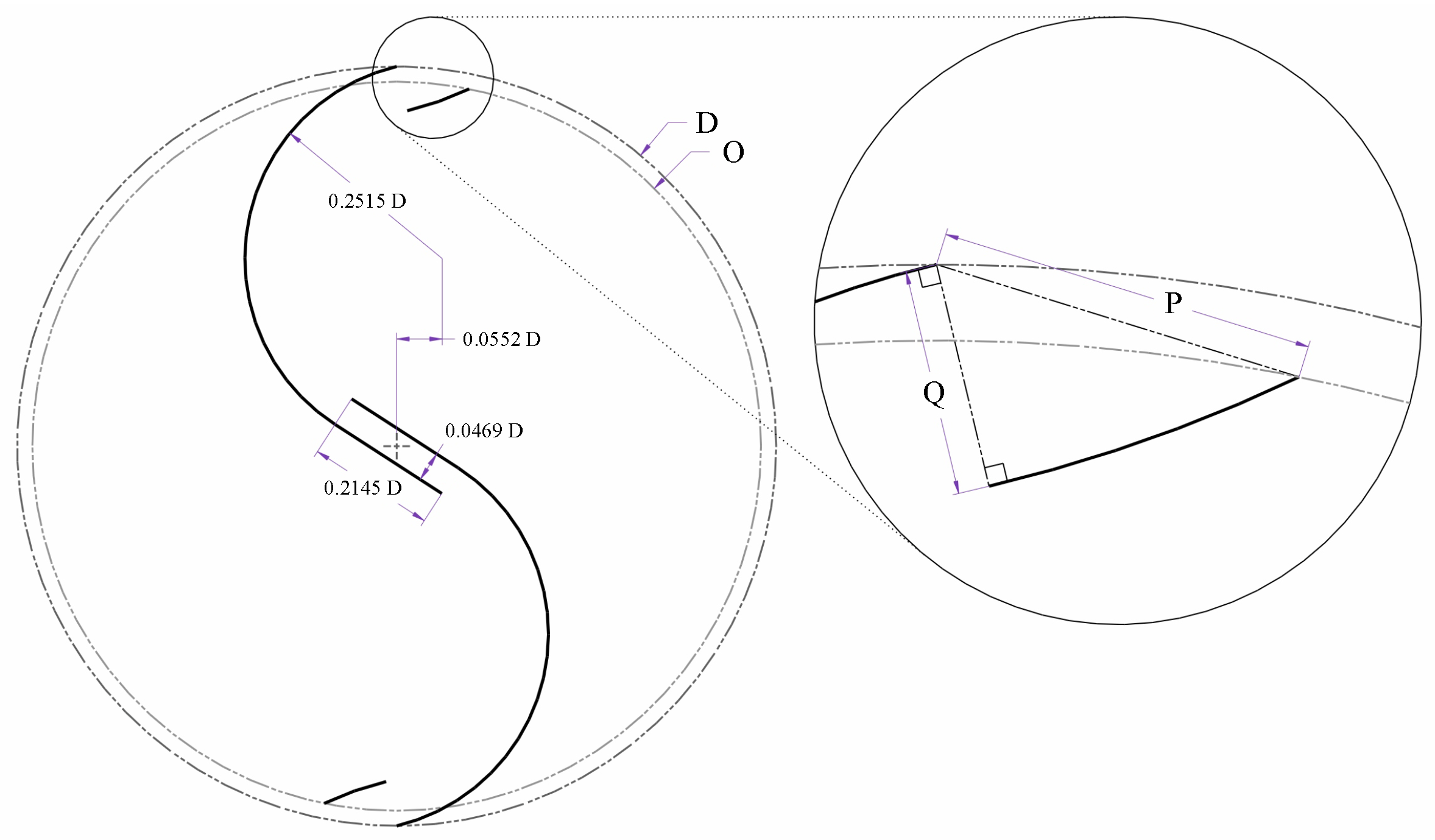
For this, three factors were established; one of them corresponds to the diameter that constitutes the leading edge of the secondary element (O) and the remaining ones comprise the distances between the leading (P) and trailing (Q) edges of the blade studied with respect to the edge outside the main element, as shown in Figure 1. These factors are dimensioned according to the percentage represented respecting the rotor diameter (D). Three levels were defined for each factor constituting an experimental design (i.e., three levels for the three factors). Table 1 shows the factors and levels used in the experimental designs.
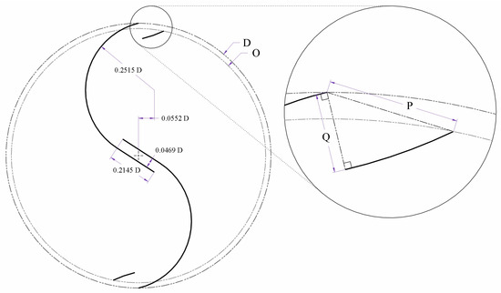
Figure 1.
Geometric parameters used in experimental designs.

Table 1.
Description of the experimental designs ().
The radius of the secondary element is obtained by construction, so that the angle at the trailing edge of the secondary element is ensured to be coincident with the angle of the outer edge of the main element. The wind velocity was defined as a constant, with a value of 4 m/s.
A FCCD does not require all the level combinations that a FFD requires, but only the central combinations between each pair of factors. In this regard, for the case of a design with 3 factors evaluated at 3 levels, a cubic structure is obtained with points of analysis at each vertex, at the center of the faces, and at the center of the body of the experimental domain, which determines a total of 15 treatments [29].
By constructing the geometries according to the values provided by the FFD and the FCCD, it was possible to obtain a total of 27 and 15 models, corresponding respectively to each treatment (i.e., combination of levels). All geometries are bounded by a circumference of 200 mm in diameter (D) and built considering a thickness of 1 mm.
The performance of each geometry is evaluated in terms of the torque coefficient () from which the power coefficient () is determined as the response variable. The is estimated as the relationship between the torque generated by the turbine on its shaft (T) and the torque that is possible to generate under the given conditions. This can be seen expressed in Equation (1), where is the density of the air, v is the wind velocity in free flow and is the cross-sectional area of the turbine, being H its height (unitary in two-dimensional analysis).
Likewise, the consists of the relationship between the power generated by the turbine and the energy flow carried by the fluid. This can be estimated by means of Equation (2), where is the angular velocity of the turbine [30].
The speed ratio at the tip of the blade () gives a proportion of the angular velocity of the turbine in dimensionless terms according to Equation (3).
Considering that the profile and dimensions of the main blade remain fixed in this study, it is assumed that the value of corresponding to the optimal performance of each geometry studied, will also be largely conserved. Therefore, the rotational velocity and its respective are determined by analyzing the rotor whose secondary blades dimensions correspond to the central levels of the experimental designs (98, 16, and 8 for the factors O, P and Q, respectively). Said geometry is rotated at different velocities in order to describe the point of maximum performance, thus determining that the optimal conditions correspond to a rate of eight revolutions per second () ().
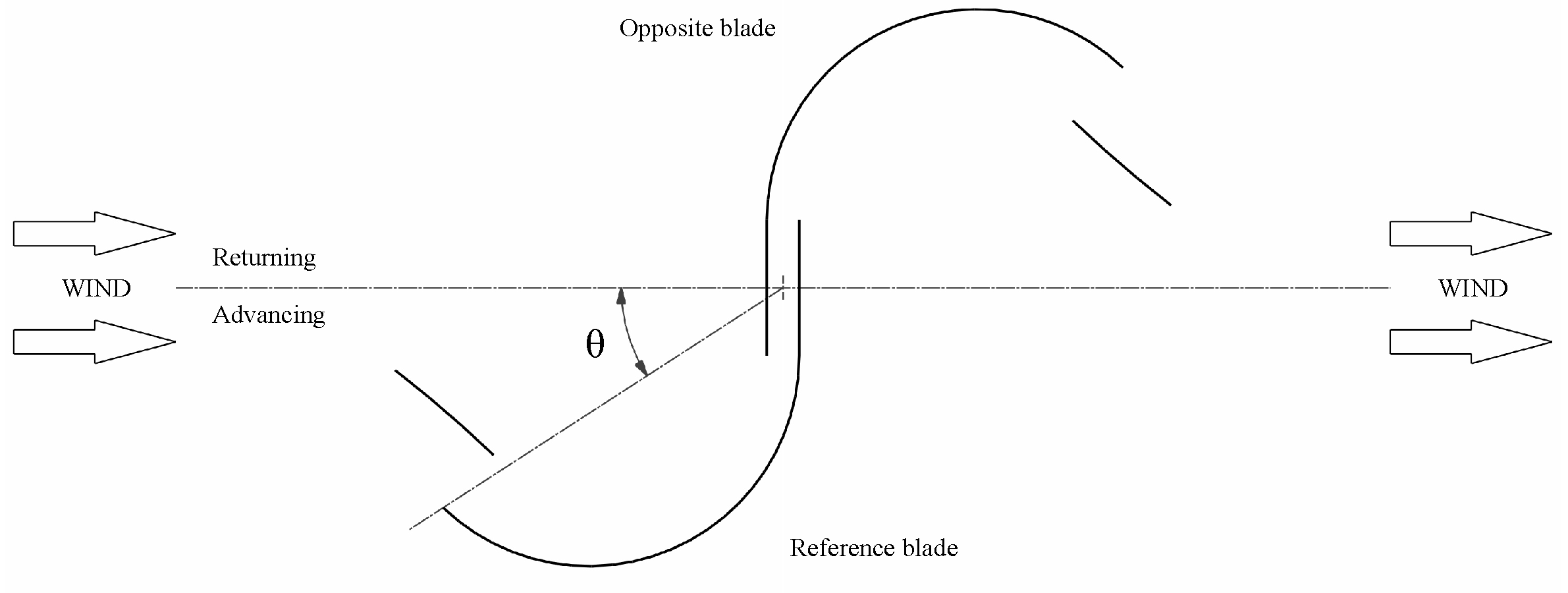
Each numerical simulation is performed for ten complete revolutions of the rotor, seeking to achieve a quasi-stable state. From the simulations, reading are taken from the generated on the rotor axis for each angular position recorded according to its azimuth angle () (Figure 2).

Figure 2.
Reference system used for the analysis of geometries.
These values are averaged for the rotor’s last two complete revolutions, corresponding to the results with the greatest temporal stability. This averaged allows us to estimate the averaged through Equation (4). This is done with all geometries, obtaining the corresponding to each combination of the experimental designs.
2.2. Specification of the Numerical Analysis
In this study, the geometries are analyzed under two-dimensional models, assuming that the rotor aspect ratio () is greater than or equal to the unit [31]. All geometries are analyzed in transient regime, under the same algorithms, parameters, and models of computational fluid dynamics (CFD) through the ANSYS Fluent software. The turbulence model is proposed for its good performance in predicting free flows and adverse pressure gradients [32,33,34]. A coupled scheme was selected for the pressure-velocity coupling algorithm and an implicit transient first-order formulation was used.
The analysis domain is made up of two parts: a rotating circular region and a stationary rectangular region. The circular region contains the profile under study and rotates constantly at the determined velocity (). The rotating circular region is divided by a sliding interface, whose diameter does not significantly influence the results. However, a prudent distance is sought with respect to the walls of the geometry so that the high gradients that occur there due to the boundary layer phenomenon do not have to be divided into different regions.
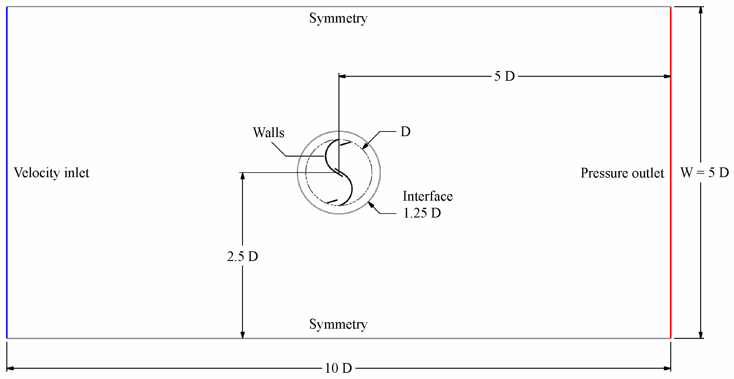
An air inlet is established at a velocity of 4 m/s (class 1 wind) [35], corresponding to a flow regime with a Reynolds number of . Similarly, an output to atmospheric conditions is set and the lateral field is simulated under symmetry conditions since there are low-scale gradients [32,36] (Figure 3). However, established boundary conditions can make it difficult to deflect flow around the turbine as opposed to the restriction produced by the turbine, thus generating a blockage effect [37]. This produces an acceleration of the flow around the obstacle and means an over-prediction of the rotor’s performance [38].

Figure 3.
Analysis domain and boundary conditions.
In a two-dimensional analysis, the blockage ratio is defined as the ratio of the rotor diameter to the flow’s domain width (), so the blockage effect can be minimized by increasing the simulation domain scale with respect to rotor size [38]. Despite this, given that within the experimental designs the same boundary conditions and the same domain size will be used for all geometries studied, this does not represent a significant variation factor, so in spite of producing altered results, these will largely preserve their relationship to each other [37].
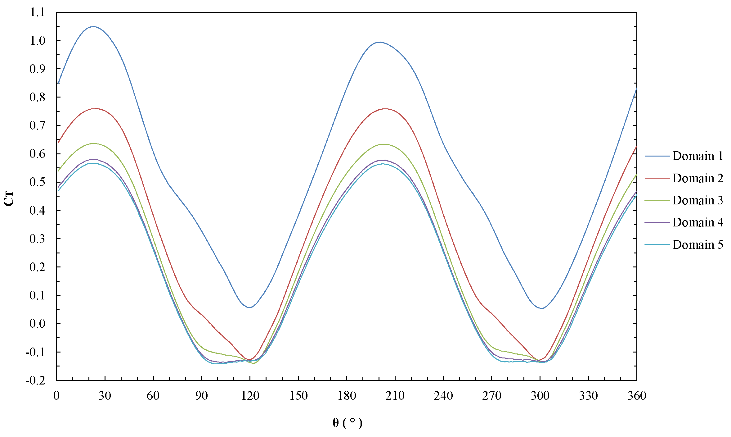
To know the value and trend of said alteration, an independence analysis is carried out for the computational domain, under the same conditions with which the experimental designs geometries are studied. The center dimensions profile is used as a test model. The results obtained in this analysis describe the behavior of according to , for each tested domains (Figure 4).
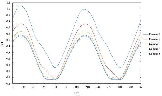
Figure 4.
Torque coefficient () according to azimuth () for each domain.
When estimating the average for each computational domain, it is evidenced that the size of the domain has a notable effect on it and that its variation becomes smaller compared with the value corresponding to the larger-scale domain (domain 5). The asymptotic convergence indicator for the domain independence analysis according to Richardson’s extrapolation is 0.9521; whose closeness to unity indicates the existence of a convergence value [39]. Table 2 shows the results obtained when testing the different computational domains.
Table 2.
Domain independence test results.
Seeking a shorter simulation time, the general dimensions of the analysis domain are established for a blockage ratio of 20% (Figure 3), similar to the study carried out by [40], so its respective deviation must be taken into account.
Similarly, to obtain an efficient number of partitions into which both the analysis geometry and the period to be simulated must be divided, it is necessary to perform a spatial and temporal discretization independence analysis, seeking to obtain a convergence in the result.
The spatial independence analysis is developed under the same conditions and for the same geometry as the domain independence analysis. Five discretizations known as meshes are built, with the same structure, but with a number of partitions according to the degree of refinement of each one.
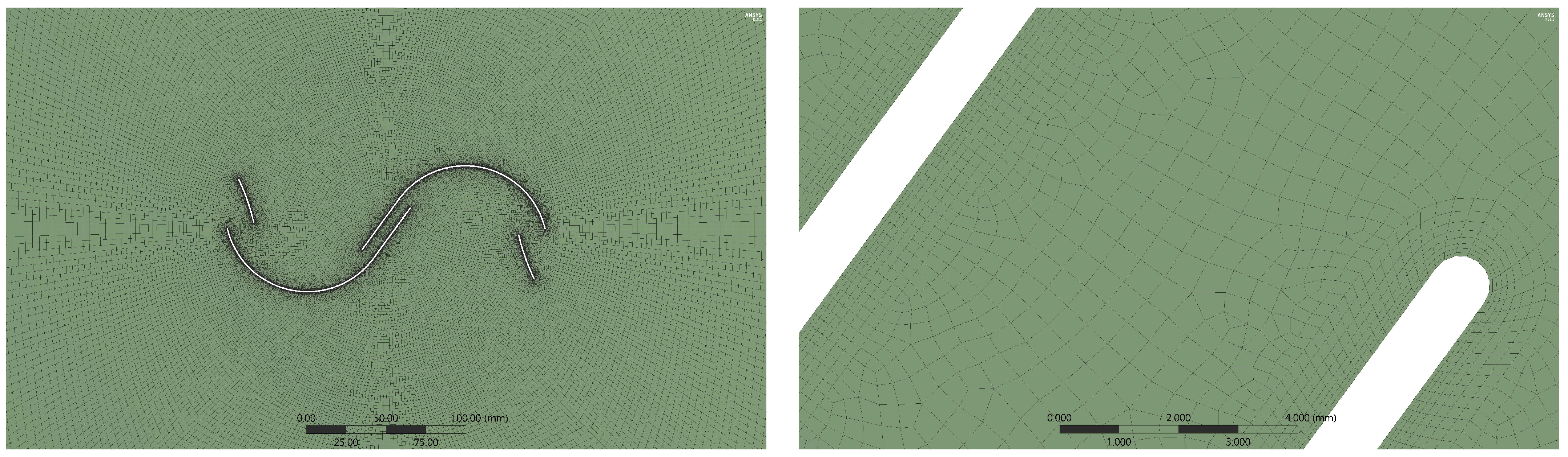
Meshing was done in ANSYS Meshing software. The static body that simulates the far fluid field has a structured mesh with only quadrilateral elements, while the mobile body that simulates the field near the rotor has an unstructured mesh with predominant quadrilateral elements and some triangular elements to achieve greater adaptability to geometry (Figure 5 left). The mesh adjacent to the rotor walls is refined and has a perpendicular layer structure (inflation) that allows a better prediction of the boundary layer (Figure 5 right).
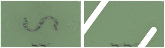
Figure 5.
General structure of the mesh (left) and details of the mesh near the profile walls (right).
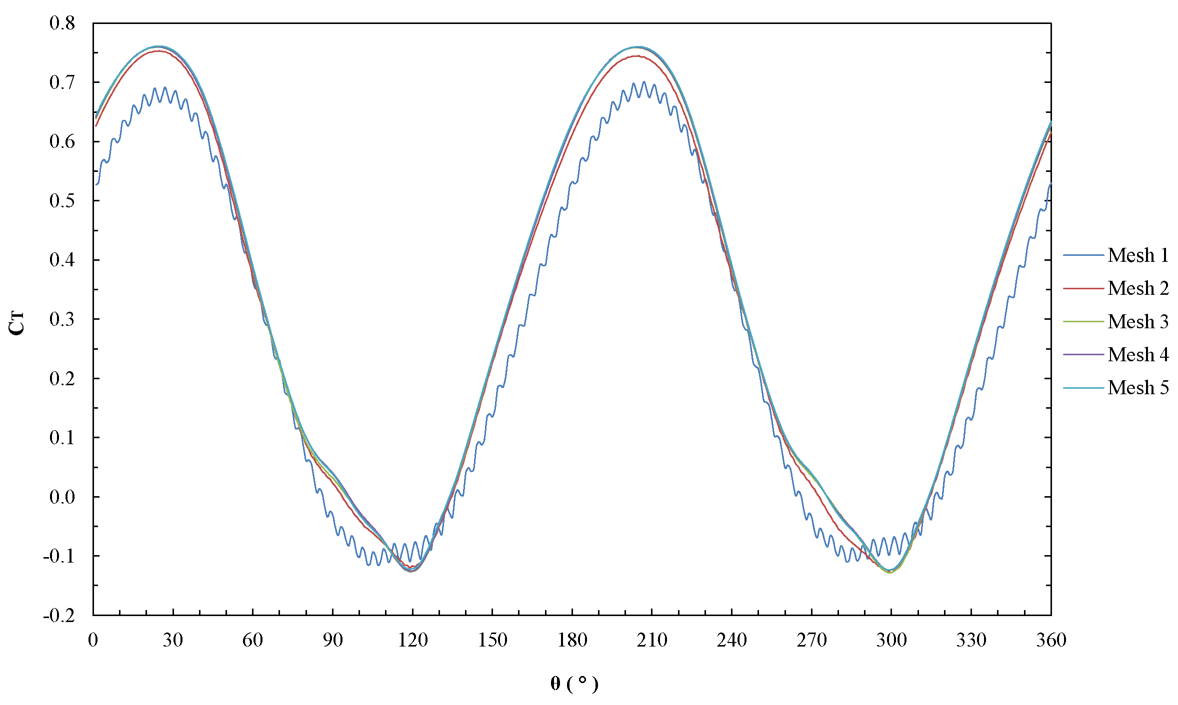
The results obtained in this analysis are shown in Figure 6 and allow estimating the averaged for each mesh. It is observed that the variation of the averaged is minimal when compared with the corresponding value of the finest mesh, thus generating an indicator of asymptotic convergence of 1.0122 according to the Richardson’s extrapolation (Table 3).
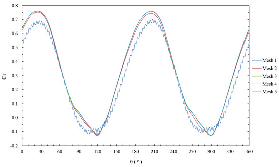
Figure 6.
Torque coefficient () according to azimuth () for each mesh.
Table 3.
Mesh independence test results.
When using the turbulence model, it is recommended that the value of be less than unity to ensure proper predictions in the flow near the walls [32,36]. For this reason, the fourth mesh is selected, which also requires a much shorter simulation time than the finest mesh (Table 3).
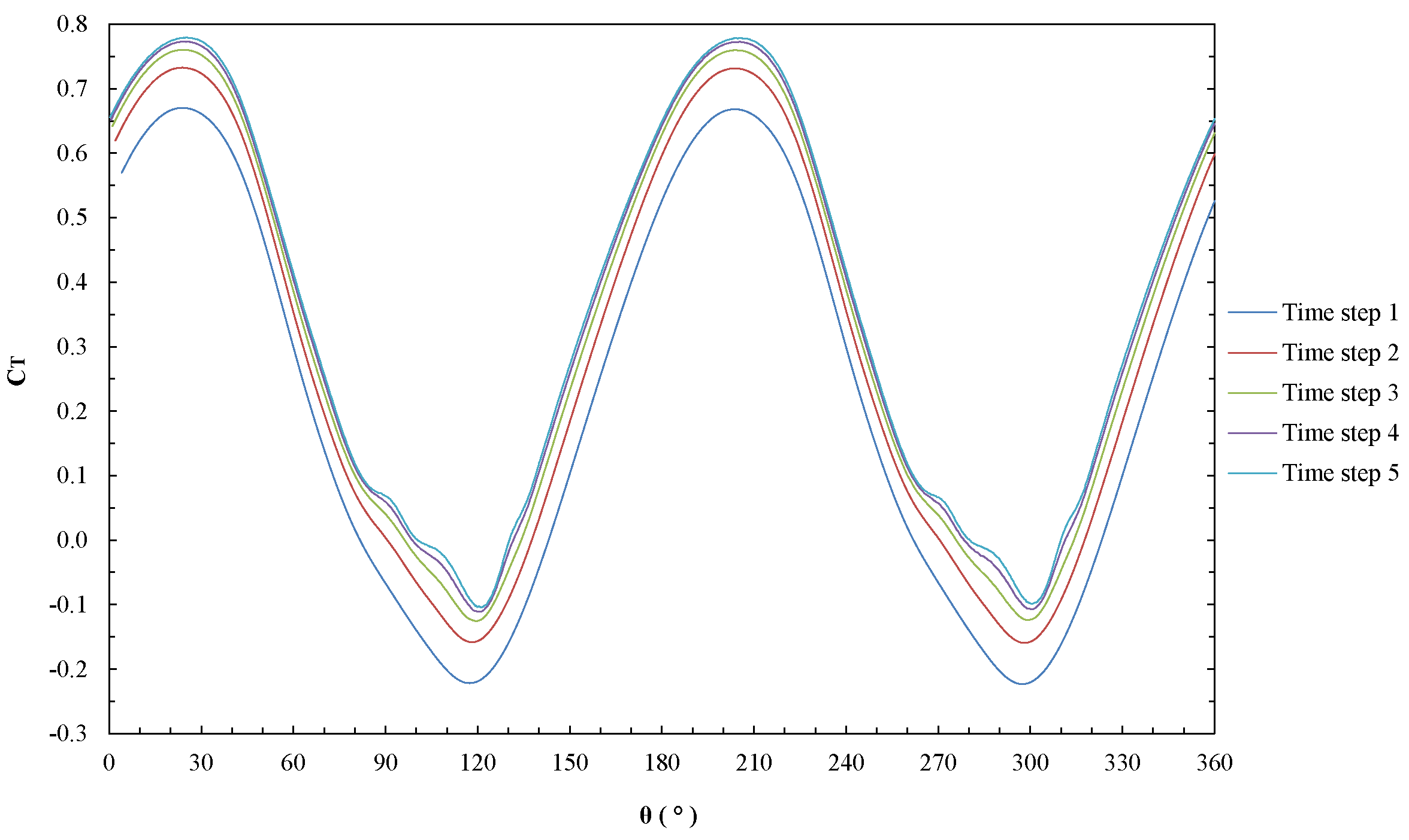
Starting from the fourth meshing, the temporal discretization independence analysis is carried out in the same way, under the same conditions, and for the same geometry as the meshing independence analysis. Five time discretizations are taken, generated by dividing the period of the rotor’s revolution into a number of elements or time steps. The results obtained in this analysis are shown in Figure 7 and allow estimating the average value of for each temporal discretization (Table 4). It is evident that the variation of the averaged decreases as the partition tightens, getting closer and closer to a convergence value that is supported by an asymptotic convergence indicator of 1.0281 for Richardson’s extrapolation. A discretization of 720 time steps per revolution is then determined, which represents a suitable relationship between the allowable error and the simulation time.
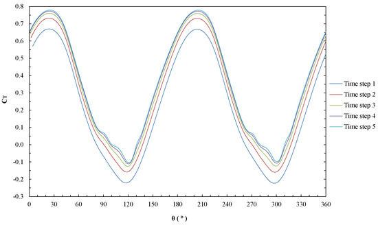
Figure 7.
Torque coefficient () according to azimuth () for each time step.
Table 4.
Temporal independence test results.
2.3. Specification of the Experimental Setup
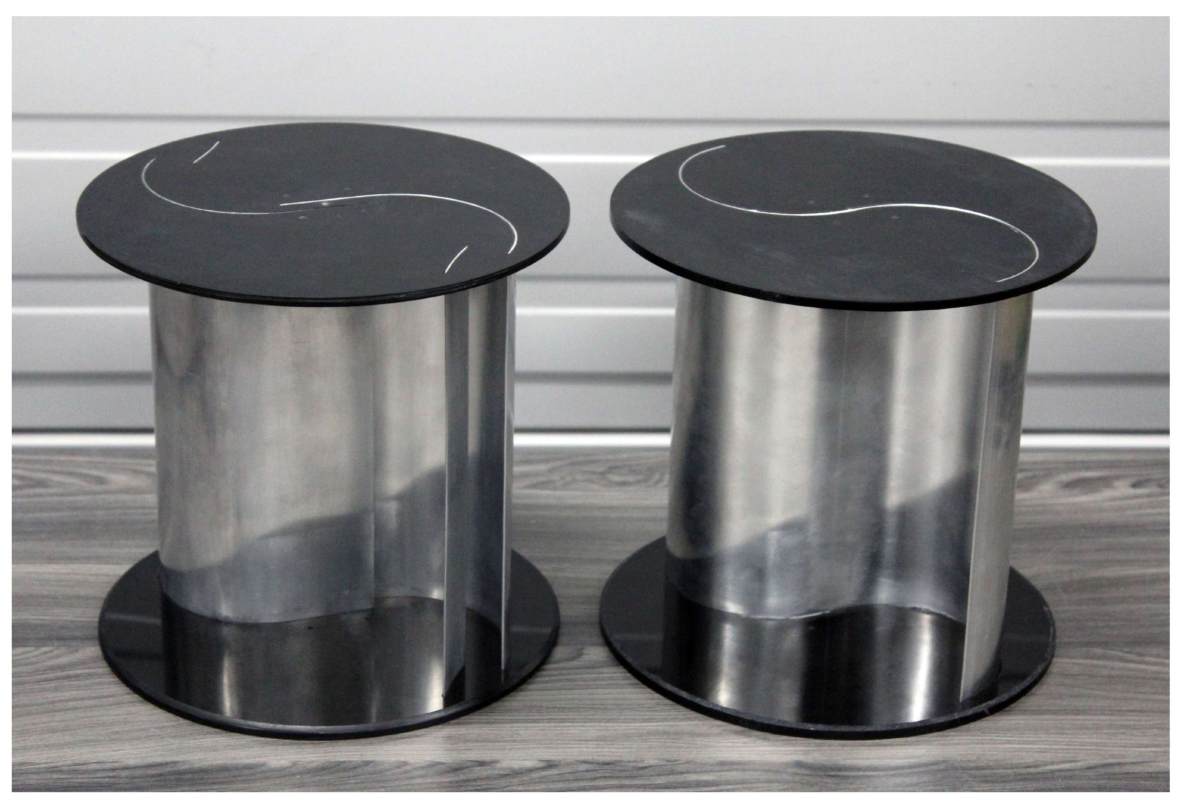
To verify the results obtained numerically, an experimental study was carried out in which the conventional semicircular profile, the split Bach profile, and the multi-blade Bach profile were evaluated using a wind tunnel (Figure 8).
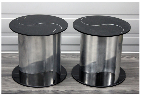
Figure 8.
Test rotors of the conventional semicircular profile (right) and multi-blade Bach (left) (the secondary blades were installed on the split Bach profile rotor model).
The study was carried out in a closed test section of 50 cm 50 cm, with a rotor model of 200 mm in diameter and 200 mm in height, corresponding to a blockage ratio of 16% (Figure 9). Plates were installed at the ends of the rotor with a diameter of 220 mm made with 6 mm thick acrylic [41]. The blades on the models were made from 20-gauge aluminum sheet. The experiment was carried out in the city of Medellín, Colombia, with an approximate air density of 1.058 kg/m, corresponding to a height of 1500 meters above mean sea level (MAMSL) (ISO 2533).

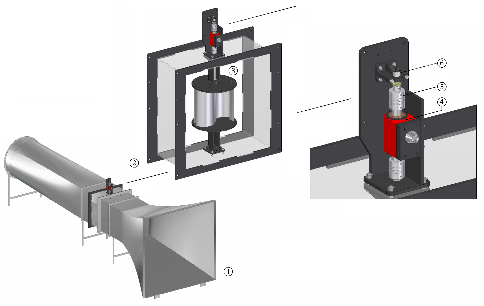
Figure 9.
Schematic of the experimental setup: (1) wind tunnel, (2) test section, (3) test model, (4) torque sensor, (5) couplings, and (6) braking electric motor.
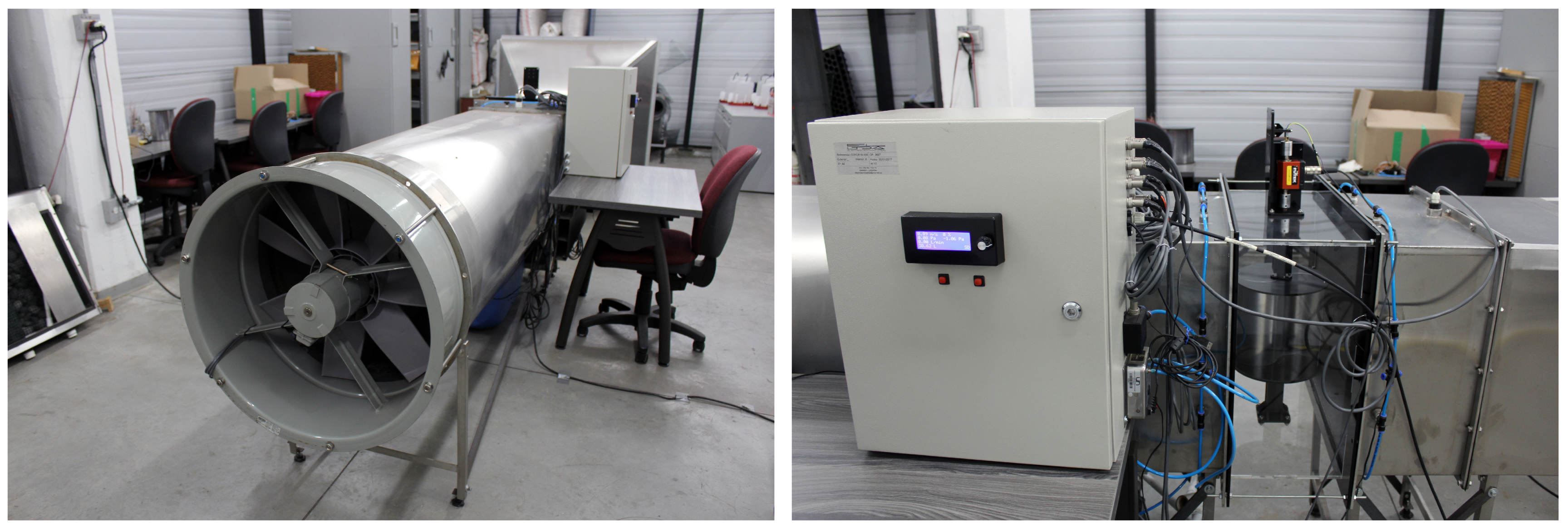
The test consisted of allowing an established air flow at a velocity of 4 m/s through the wind tunnel (Figure 10). The flow velocity was adjusted through an ultrasound anemometer located m upstream of the rotor, before conducting each test. This was withdrawn again to avoid disturbance of the incident flow on the rotor.

Figure 10.
Wind tunnel used for experimental development (left). Detail of the experimental setup and the measurement system (right).
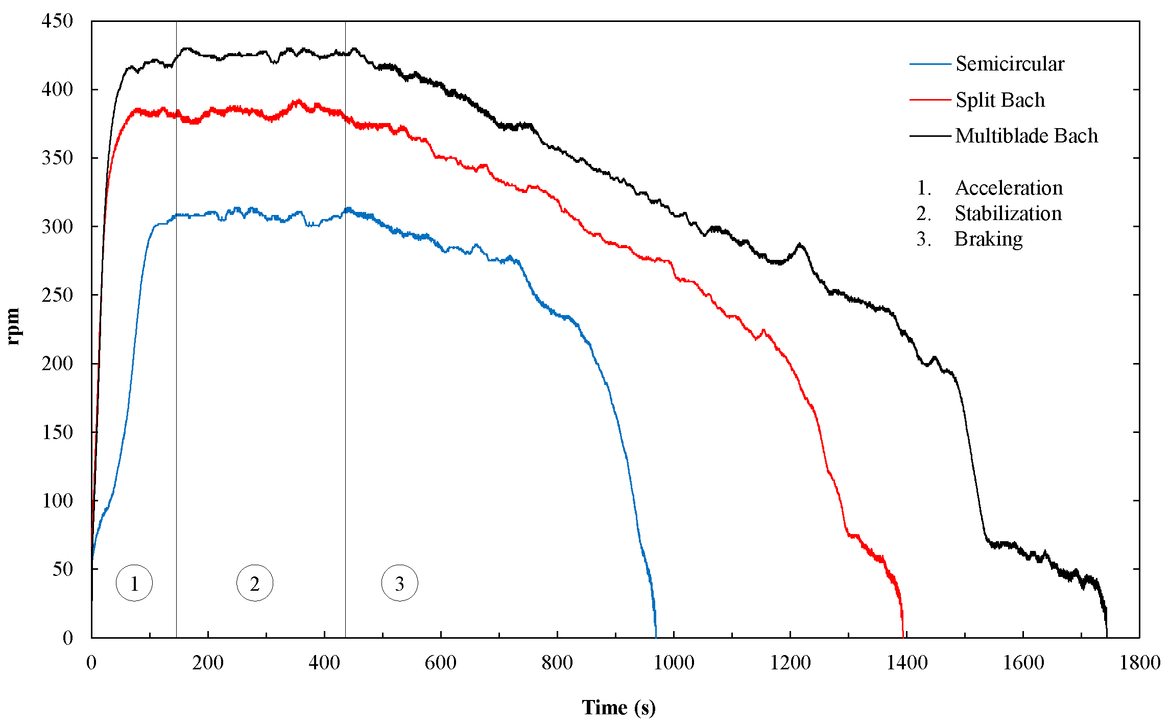
The flow inside the tunnel accelerated the rotor from zero velocity to its limit velocity without load. Once the rotation regime stabilized, a power signal was sent to an electric motor, which was constantly increasing its intensity. The load exerted by said motor made the test rotor brake until it was completely blocked (Figure 11).
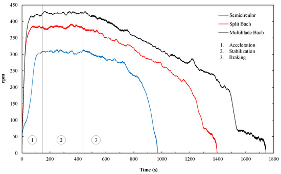
Figure 11.
Velocity during tests histogram.
Measurements were made using a torque sensor with encoder and a control system that allowed modifying the load exerted by the electric motor from the pulse width modulation (PWM) in its power signal, regulated at V.
The purpose of the experimental study is to validate the results obtained from the numerical analysis rather than to approximate the real performance of the rotor. Therefore, in order to compare the results obtained experimentally with the numerically estimated data, it was necessary to replicate the experimental conditions within a three-dimensional numerical model formulated according to the system’s degrees of freedom (6-DOF solver). In this regard, the blockage ratio within the wind tunnel does not represent a variation factor between both approaches.
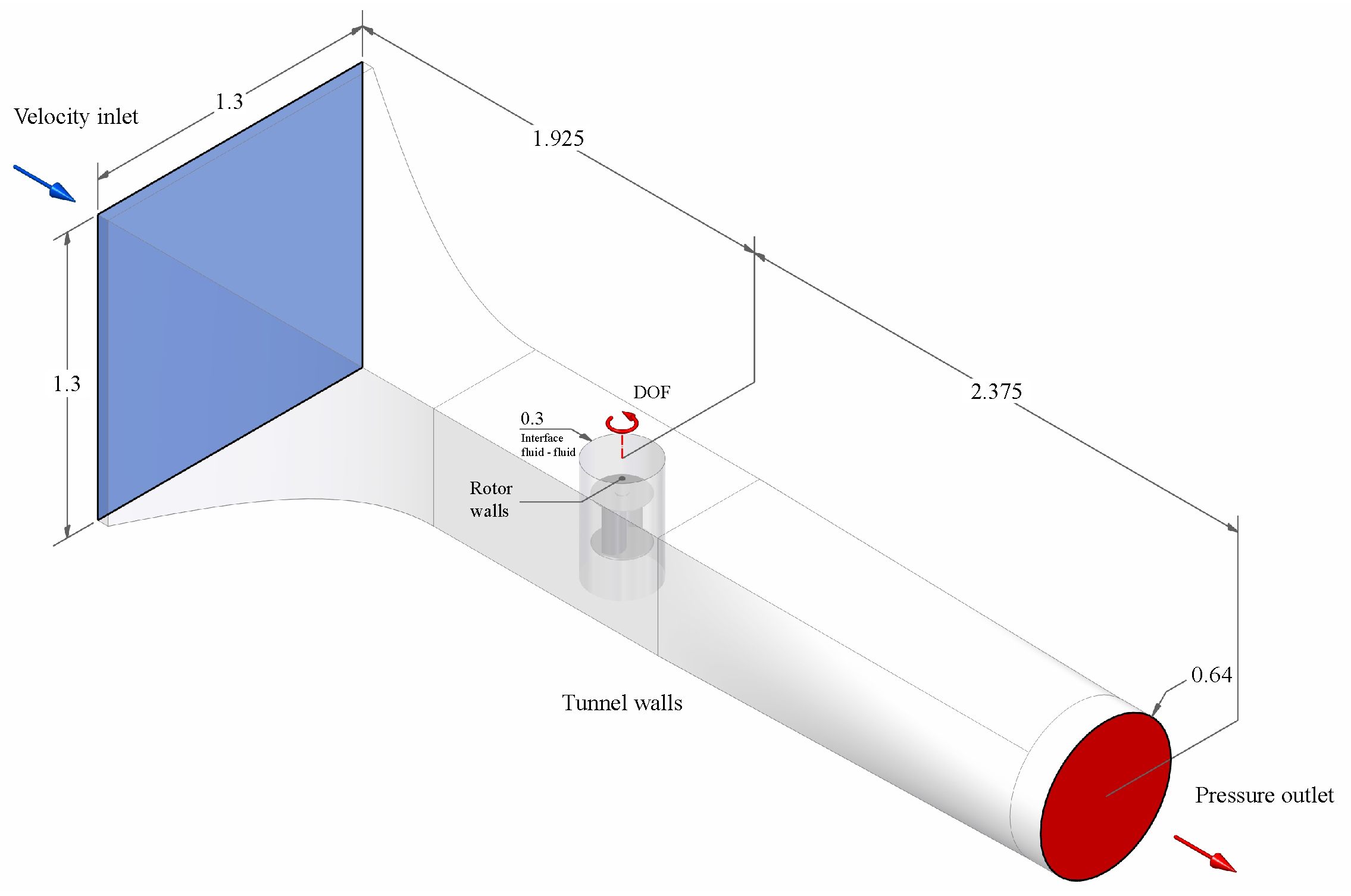
For this, the same conditions with which the two-dimensional models were studied were established, in addition to assigning the required degree of freedom to the turbine’s axis of rotation (Figure 12. In the same way, the spatial and temporal discretization independence analysis was carried out, stabilizing the results, and obtaining an efficient discretization of elements and a time step of s (Figure 13).

Figure 12.
Domain size and conditions of the three-dimensional numerical analysis.
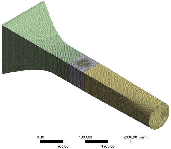
Figure 13.
General structure of the mesh.
3. Results
3.1. Hypothesis Testing
The values obtained from the simulations must fit a normal distribution to guarantee the regression’s model validity. Additionally, the residuals obtained from the regression must be random, normally distributed, and must have a constant variance, respecting each factor (homoscedasticity). Normality in the response variable is verified with the Kolmogorov–Smirnov and Shapiro–Wilk tests, and normality in the residuals is verified with the Jarque–Bera test. Likewise, the assumptions of independence and homoscedasticity in the residuals are verified under the Wald–Wolfowitz and Levene tests, respectively [29].
The statistical analysis is developed through the software R 3.6.1. For each one of the two experimental designs, a second-order multiple regression model is fitted with interactions [29]. When performing the hypothesis tests on each regression models, their plausibility is evaluated, establishing a 95% confidence for their fulfillment, which corresponds to a minimum significance level of 0.05. As can be seen in Table 5, the p-values of the tests are greater than the established level of significance, so the hypotheses that lead to compliance with the requirements cannot be rejected.
Table 5.
Results of the tests in the adjustment of the regression model for the FFD and the FCCD.
3.2. Response Surface
The results of the numerical simulations for each treatment of the FFD are shown ordered according to their factors in Table 6 and for each treatment of the FCCD in Table 7.
Table 6.
Power coefficient () determined for each treatment of the FFD.
Table 7.
Power coefficient () determined for each treatment of the FCCD.
The results of the Fisher test F global allow one to conclude with full confidence that the analyzed data respond to a trend and, therefore, can be modeled (p-value = 1.332 for the FFD and p-value = 3.9 for the FCCD). A second-order multiple regression model with interactions is adjusted for each experimental design, with which the effect of the different factors is determined. The null hypothesis of the test establishes that the analyzed factor has no effect on the response variable. Therefore, the lower the p-value of each coefficient, the greater the evidence against the null hypothesis, suggesting a significant difference generated by the respective factor [42]. Table 8 summarizes the results of the variance analysis (ANOVA) for the adjustment of the regression models of the FFD and the FCCD.
Table 8.
ANOVA for the regression models adjusted for the FFD and the FCCD. (DOF), (SS), and (MS) refers to degrees of freedom, sum of squares, and mean squares, respectively.
Table 9 shows the test statistics for each factor and experimental design results.
Table 9.
Test statistics for each factor and experimental design results.
The coefficients that correspond to each factor constitute the regression polynomial that determines the value of the response variable in each coordinate [43]. Equations (5) and (6) express the regression polynomials for the FFD and the FCCD, respectively.
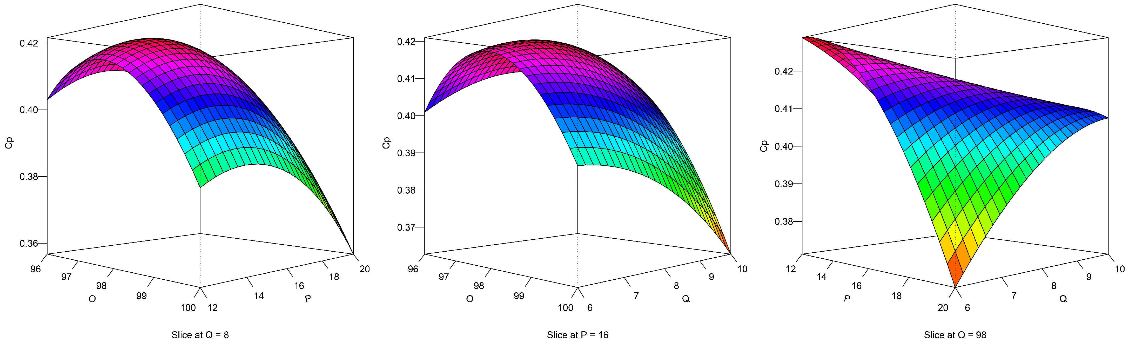
Figure 14 shows the surface graphs obtained by evaluating the FFD’s regression polynomial as a function of two factors. The surface graphs of the FCCD’s regression polynomial are appreciably similar.

Figure 14.
Response surfaces perspective graphs.
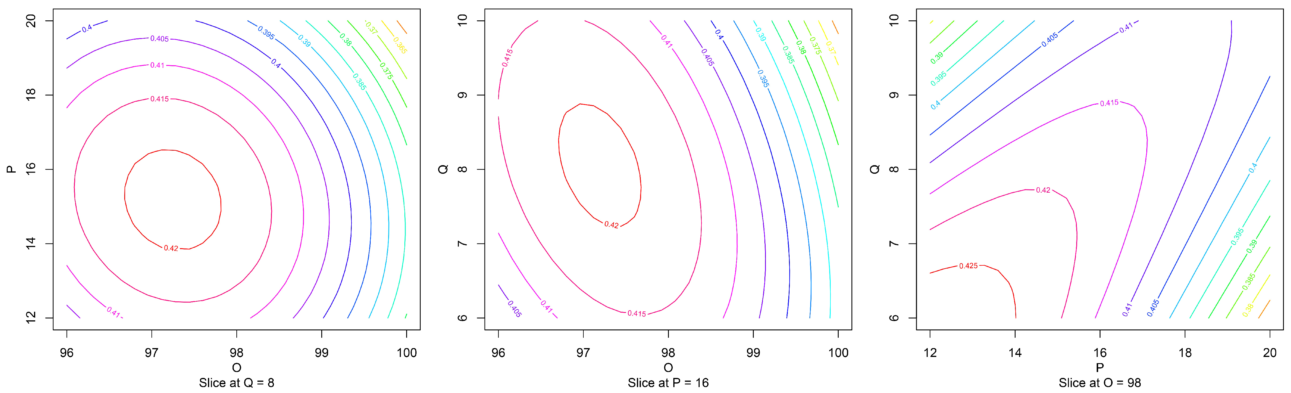
To determine the geometric proportions that allow the maximum performance, the point at which the derivative value of the regression polynomials becomes zero must be found. Figure 15 offers a better appreciation of the surfaces stationary points shown in the previous figure.
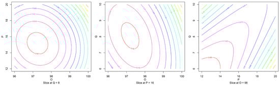
Figure 15.
Response surfaces contour graphs.
The coordinates of the global stationary points for each experimental design, in which all the factors of each model simultaneously have zero slope, are comparatively shown in Table 10. Substituting these coordinates in each regression polynomial results in a modeled . Likewise, when constructing the profile with the optimal proportions and simulating it under the same conditions with which the geometries were simulated previously, a numerical is obtained. These optimal performance values are exposed in the same way in Table 10.
Table 10.
Comparative between the FFD and FCCD designs.
Table 10 shows a significant decrease in the number of treatments required by the FCCD respecting the FFD, which means a reduction in resources of 44.44%. Additionally, the estimated through these models largely preserves its order of magnitude.
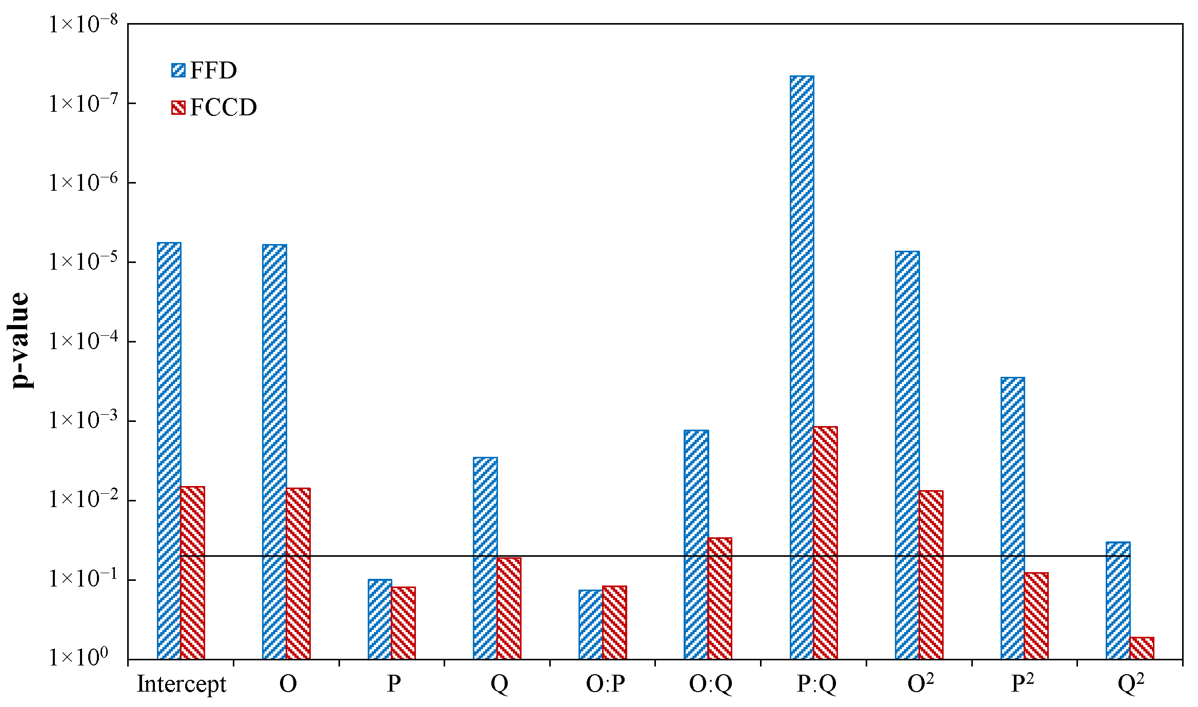
However, the optimal points estimated through the regression models of each design show significant differences, mainly in the P and Q factors. Likewise, when simulating the geometries built from these optimal parameters, the FFD presents a more favorable result in performance, which leads to a greater acceptance of this model for the purposes of this research. On the other hand, although the goodness of fit () is higher for the FCCD with a difference of 2.76%, the adjusted is 0.52% lower, which reveals a greater effect of the factors on the response variable in the FFD than in the FCCD. This can be verified in Figure 16, where a supremacy in the scale of the effects of each factor and their interactions is identified, indicating that it is possible to capture more information from the data in the first design than in a second. This may be the root cause that the prediction of the optimum point in the FFD is more accurate.

Figure 16.
Significance level for the different factors and interactions in the FFD and FCCD designs (the black line represents the maximum significance level of 0.05).
The linear and quadratic effects of the O factor correspond to those with the lowest p-values among the main and second-order effects, respectively; this indicates greater evidence of presenting the greatest effect on the response variable with respect to the other terms of the same order. These results also show that its effect on the response variable is offered individually to a greater extent, without substantially depending on the magnitude of the other factors.
The same occurs with the interaction , whose p-values close to zero, demonstrates the great dependence that exists between both factors and their significance within the model. This result confirms the importance of analyzing the factors together in order to consider the variation of each of them, respecting the variation of a second factor. On the other hand, the curvature implied by the significant quadratic effects, validates the implementation of the second-order model for adjusting both experimental designs.
3.3. Experimental Results
After recording the rotation velocity and the torque exerted between the rotor and the braking electric motor, the power generated for each recorded instant () was calculated. Finally, the average of the torque and power values corresponding to the same rotation regime was determined and it was carried to dimensionless terms (Figure 17 and Figure 18).
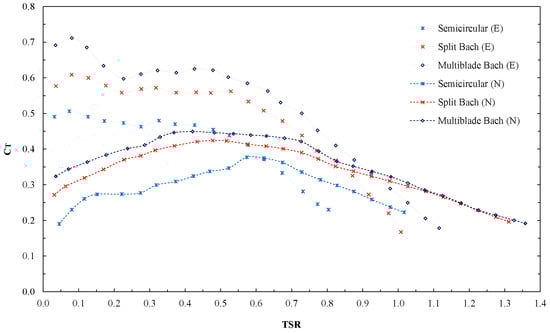
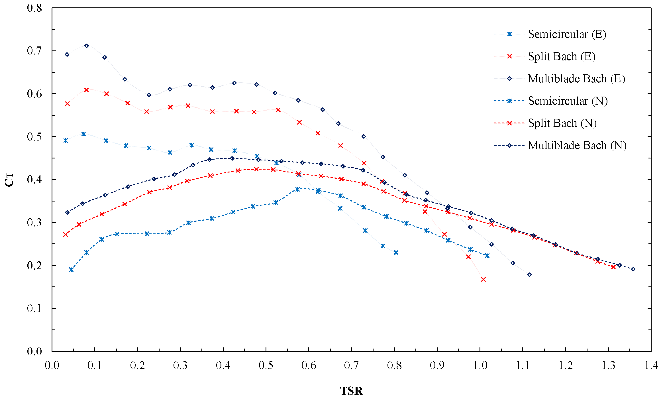
Figure 17.
Results of obtained experimentally by the three tested rotors (E) and their comparatives with the numerical results determined from the three-dimensional simulations (N).
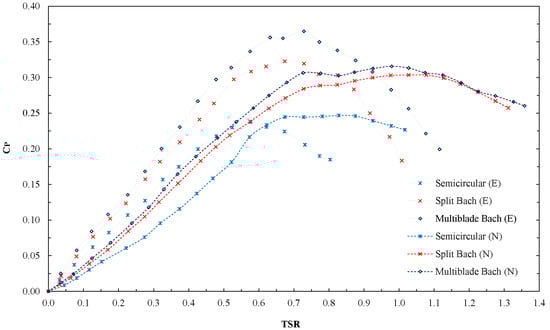
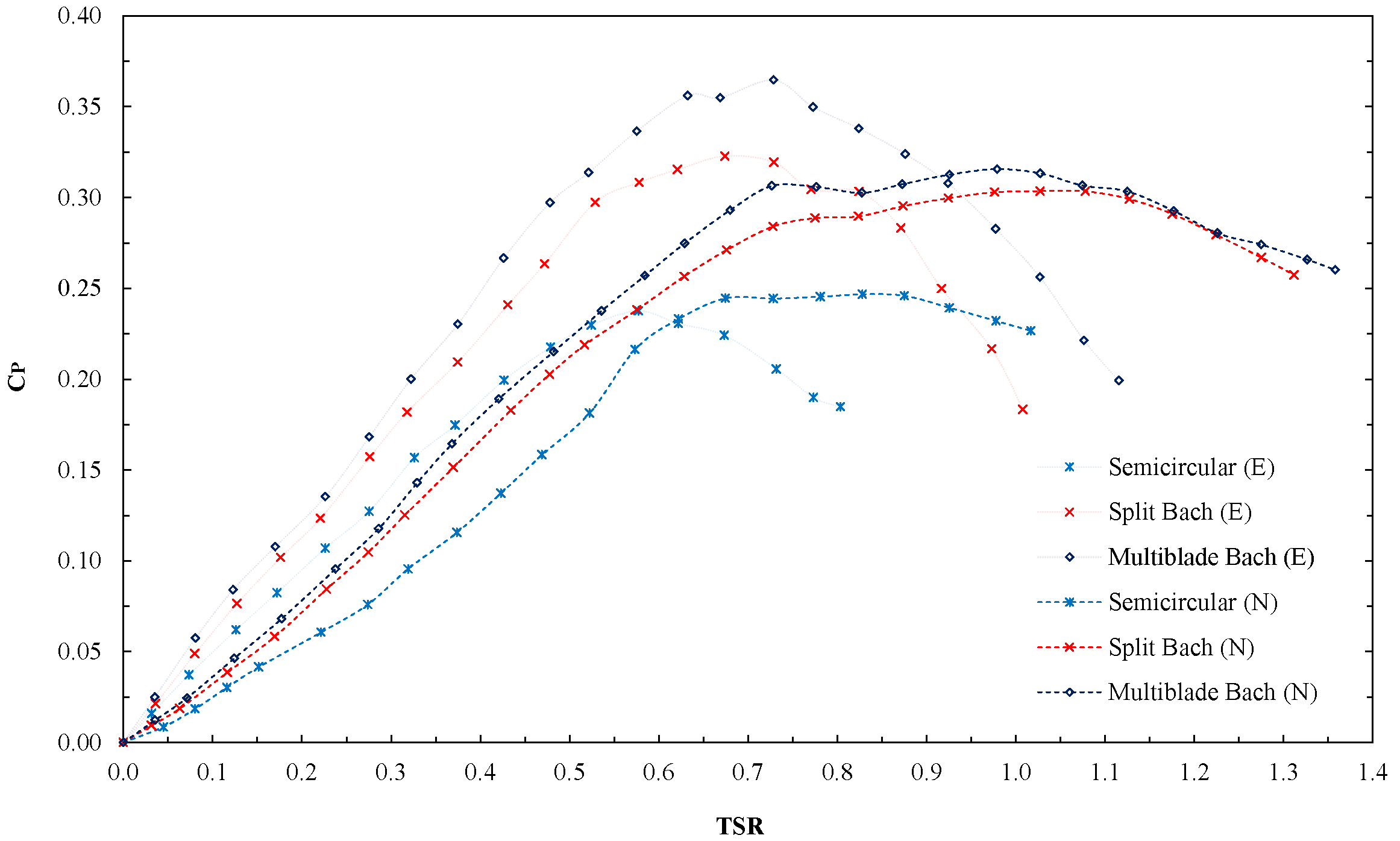
Figure 18.
Results of obtained experimentally by the three tested rotors (E) and their comparatives with the numerical results determined from the three-dimensional simulations (N).
Since the numerical and experimental data were obtained in test sections with the same blockage ratio, any source of variation between both approaches should not be found.
In Figure 17, it can be seen that the curves conserve their order of succession of the three rotors in each approach, with the multi-blade Bach profile being the one with the highest performance both in the numerical and in the experimental one.
Similarly, in Figure 18, it can be seen that the relationship between the results of of the three rotors is significantly conserved within each approach, revealing that the difference between the multi-blade Bach profile and the split Bach profile is about half the difference between the latter and the conventional semicircular profile.
The differences presented between the results of the numerical study and the experimental one may be mainly due to friction. In the simulations, the rotor turns freely and the effects of the supports are neglected, which causes a reduction in the angular velocity and, consequently, modifies the values of the at which the different characteristic points are achieved in the rotor’s performance curves.
Similarly, when the rotor attempts to come to a complete stop, the transition that occurs between dynamic and static friction at the point of imminent movement generates slight torsional pulses on the sensor shaft that alter measurements and cause values to be recorded; the torque increased to low (Figure 17).
Moreover, the roughness on the blades surface affects the relationship between the aerodynamic coefficients of the profiles , causing performance to decrease [44]. In the numerical study, smooth rotors were evaluated, but during experimentation, the models were used, although they had a good surface finish, they were not ideal.
On the other hand, considering that the wind velocity is the variable with the greatest significance in the estimation of rotor performance, because it is at the third power, any minimum deviation (either due to calibration or resolution of the measuring instrument, or because the presence of the instrument may alter the flow conditions within the tunnel), may be magnified and affect the performance measurement appreciably.
4. Discussion
4.1. Performance Analysis of the Optimized Profile
To obtain a better estimate of the actual turbine performance, the simulation of the optimized rotor is performed using a larger scale simulation domain. A square domain whose side is 50 times the diameter of the rotor is used (blockage ratio of 2%), seeking to minimize the blockage effect produced by the rotor in the flow field. Rotors with the conventional semicircular profile and the split Bach type without secondary elements are also analyzed under the same conditions.
In this way, the rotor with a conventional semicircular profile has a of 0.195. Likewise, the geometry with the split Bach type profile without secondary elements allows reaching a of 0.2661. In contrast, the rotor with the optimized multi-blade Bach profile develops a of 0.2948, which represents an increase in its performance of 51.2% and 10.8%, respectively.
To understand the aspects that led to this result, the variations in the aerodynamic behavior of the blade when implementing secondary elements are analyzed. To do this, the in one of the blades of each rotor is determined as a function of , at a rotation velocity of 7 rps (), corresponding to the maximum performance of the Bach type profile for the 2% blockage ratio (optimal velocity decreases to convergence by reducing blockage effect). This is done under the simplification that the two blades that constitute each rotor have similar and counter-phase performances.
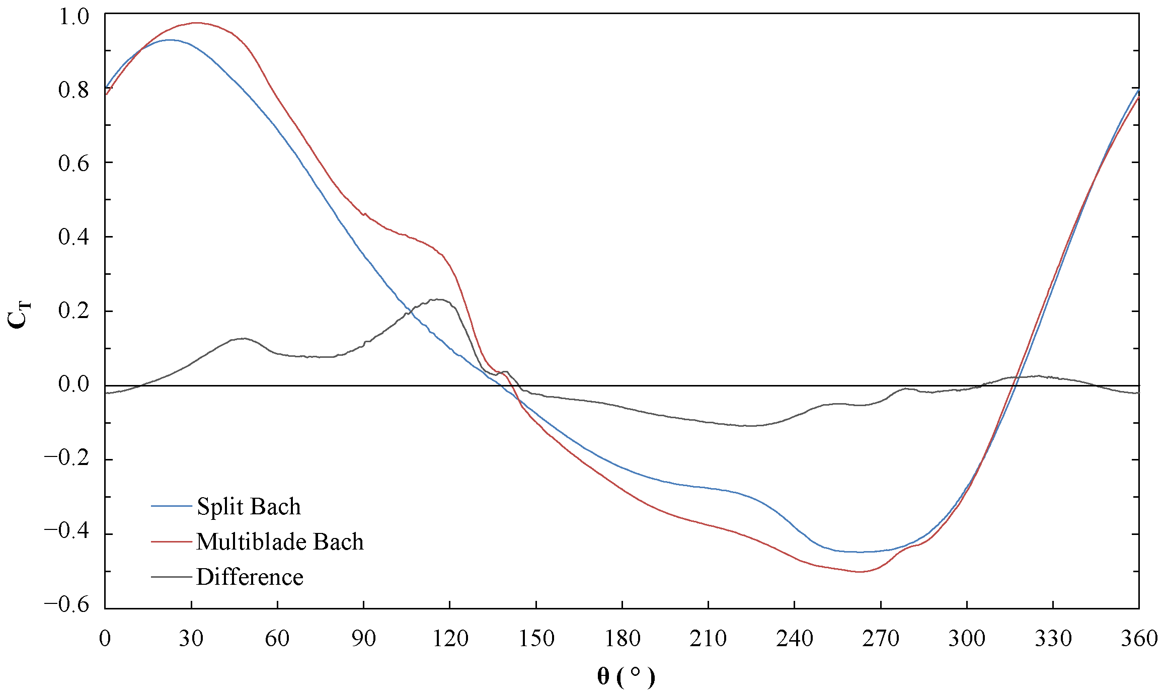
In Figure 19, it can be seen that the maximum torque from the two types of blades is obtained at the beginning of the advancing phase, in a position close to 30°, which allows to conclude that it is produced in contribution of drag force and lift force. In the same way, the minimum torque occurs during the returning phase when there is greater flow obstruction (close to 270°), which indicates that it is mainly caused by the parasitic drag force [19,23].
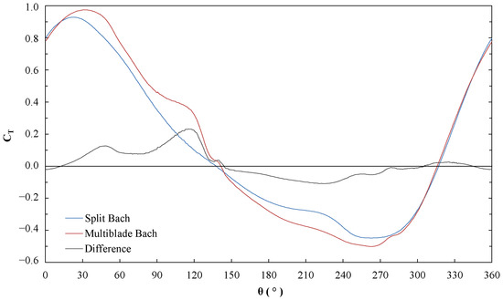
Figure 19.
Difference between the torque coefficient () in one of the blades of each rotor, at a of 1.0996.
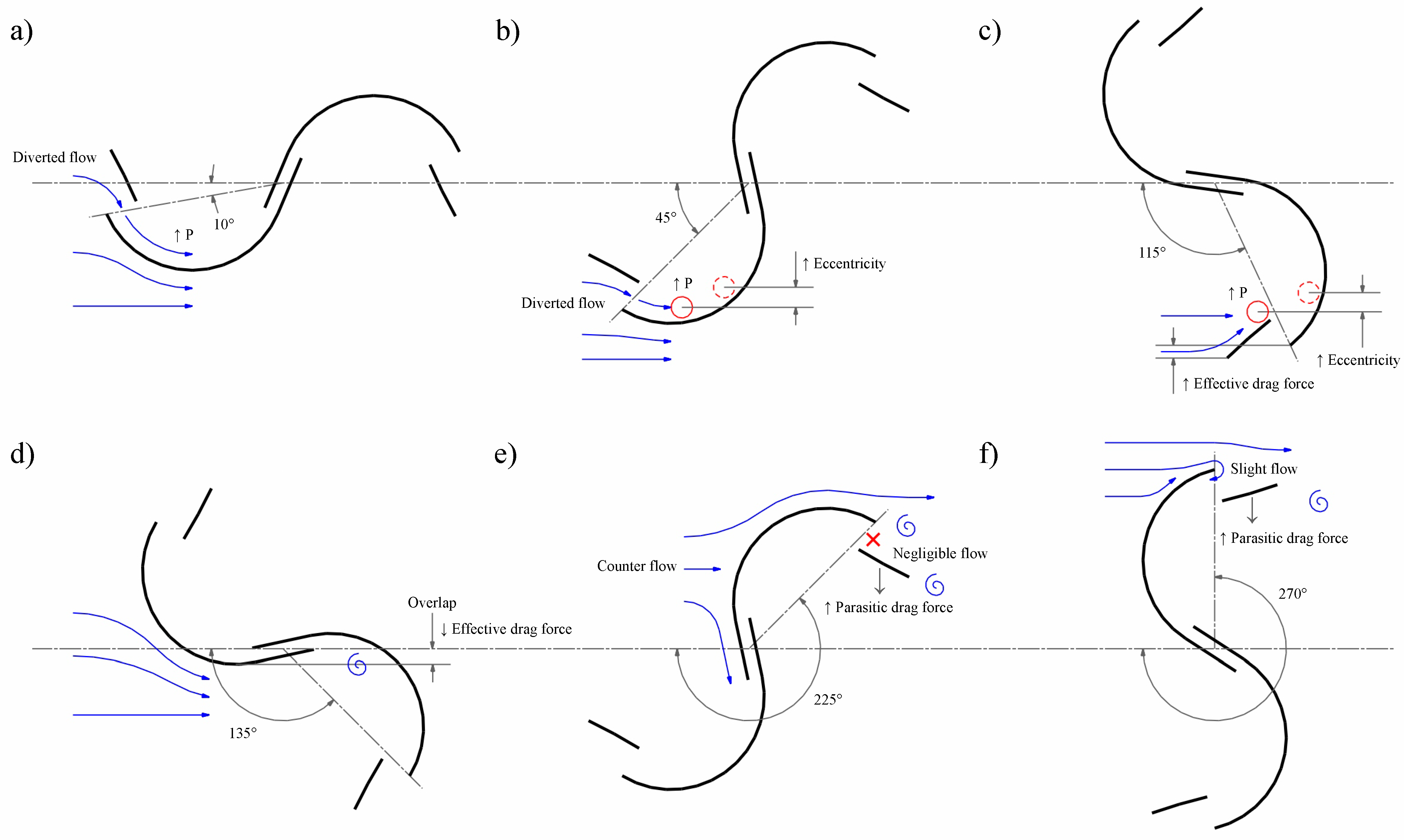
When analyzing Figure 19 in detail, it can be seen that the advantage of the multi-blade profile presents when the advancing phase begins (Figure 20a), ascending to a medium height peak generated by the greater pressure that causes the flow deflected by the secondary element toward the most extreme zone of the concavity of the main element, where, as it has a greater eccentricity, a greater torque is generated (Figure 20b). This advantage continues until the blade is aligned with the flow on its way to the rear, where the drag force and its eccentricity decrease, causing a decrease in the torque generated. During this journey, in a position close to 115°, the secondary element shows its greatest contribution by prolonging the drag force action and allowing the rotor in question to maintain a higher torque for a longer period (Figure 20c).
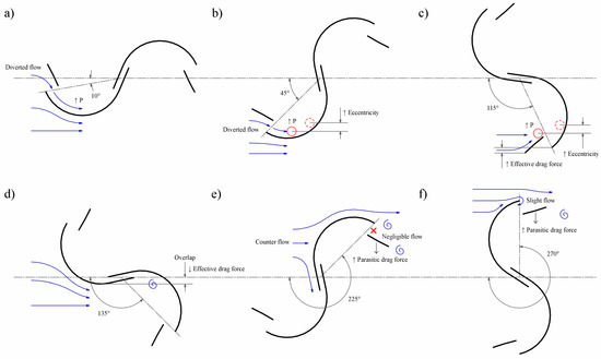
Figure 20.
Aerodynamic behavior diagram of the rotor with multi-blade profile at the significant points of performance: (a) azimuth angle () of 10°, (b) 45°, (c) 115°, (d) 135°, (e) 225° and (f) 270°.
Once the opposite blade overlaps, the flow that affects the reference blade becomes obstructed, causing it to decrease the positive torque and start to represent a load, since it requires to be moved through the fluid (Figure 20d). In this way, the reference blade travels a negative torque path that is asserted in the returning phase, when the flow incises the opposite way.
While the secondary element remains hidden from the flow, it does not show any usefulness, but it does suppose a greater resistance by having to displace a greater mass of fluid in its movement, causing a detriment in performance compared to the base profile. This disadvantage reaches its lowest point at a position close to 225° (Figure 20e).
As the blade approaches the position of greatest resistance (Figure 20f), the secondary element begins perceiving a slight flow, which, when deflecting it toward the concavity of the main element, allows it to counteract the additional resistance that this means, and makes the difference between the performance of the two profiles remain close to zero. In this way, it once again achieves a position in which it gets to divert a sufficient part of the flow to replenish with profit the losses that will be generated during the next cycle (Figure 20a).
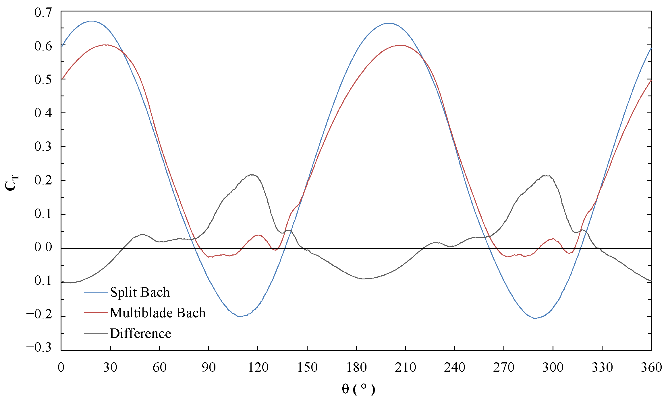
Figure 21 shows the behavior of the for each rotor, obtained from the performance sum of each of the blades that constitute them.
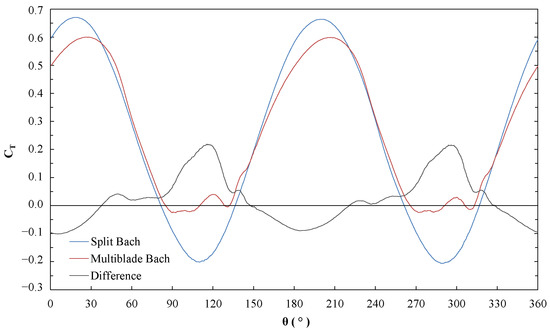
Figure 21.
Difference between the torque coefficient () of each rotor, at a of 1.0996.
As can be seen in Figure 21, the position in which the greatest performance advantage occurs between both rotors corresponds to a close to 115° (and its homologous at 295°). Likewise, the position in which the greatest decrease in performance is revealed is close to 185° (and its homologous at 5°). When comparing the graphs of Figure 19 and Figure 21, it is possible to conclude that the blades that are at the back, respecting the flow (90° to 270°), are the greatest contributors in the performance differences between both rotors.
Similarly, in Figure 21, it can be seen that the addition of secondary elements allows reducing the fluctuation in torque, partially decreasing performance at the peaks, but almost completely canceling the negative torque. Thus, the standard deviation decreases from 0.31 to 0.23, which means a reduction of close to 35%.
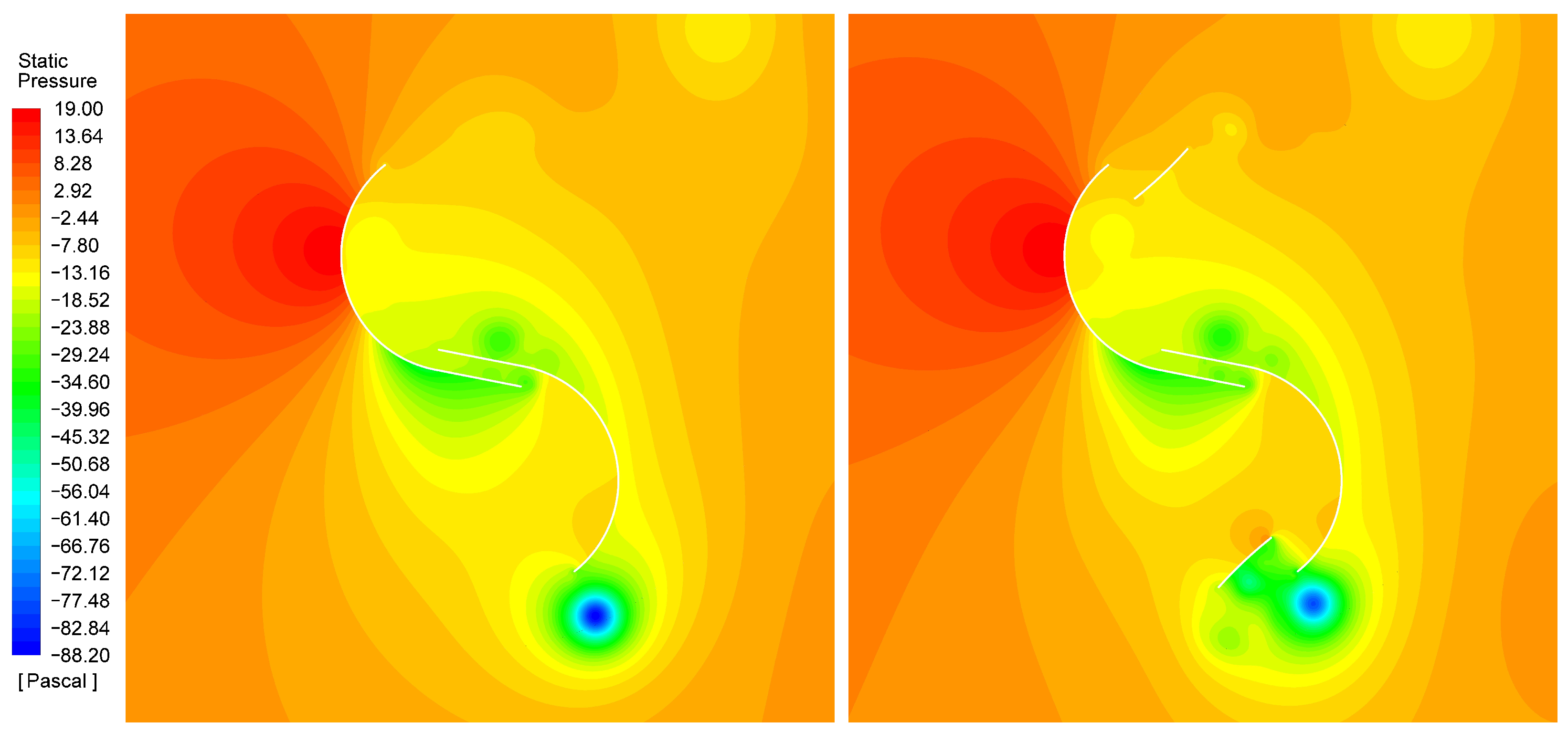
In the contour graphs, the states of pressure and flow velocity through the geometries being studied are presented. In Figure 22, it can be seen that the pressure on the concave side of the advancing blade is higher in the multi-element profile than in the profile without secondary elements, when the rotors are in the position of the greatest advantage in performance. This higher pressure also induces a slightly higher flow through the gap generated by the profile’s splitting (Figure 23).

Figure 22.
Pressure contour graphs for the split Bach profile (left) and the multi-blade Bach profile (right) at a rotor azimuth angle () of 115° and a of 1.0996.
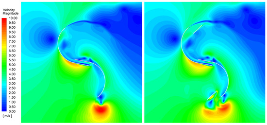
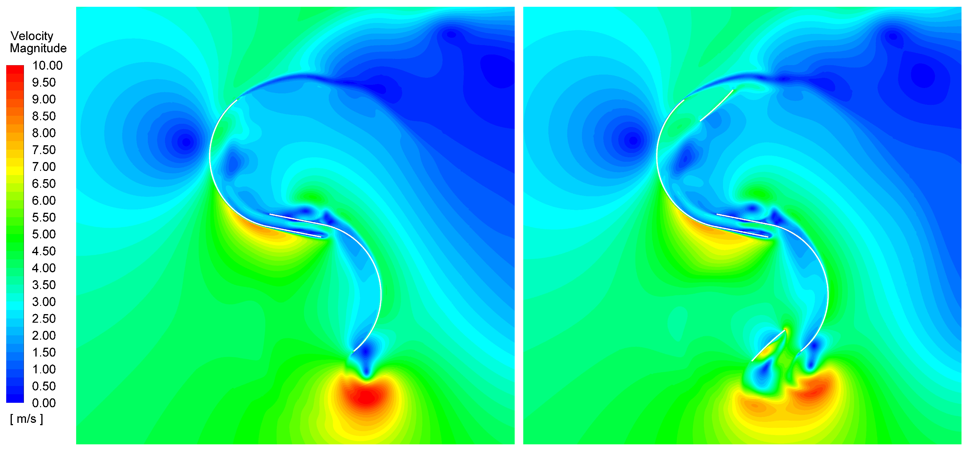
Figure 23.
Velocity contour graphs for the split Bach profile (left) and the multi-blade Bach profile (right) at a rotor azimuth angle () of 115° and a of 1.0996.
In Figure 23, a region of higher velocity can be seen on the secondary element of the returning blade, generated by the flow that deflects this surface toward the concavity of the main element, which consequently can mitigate the depressurization that is generated in this area (Figure 22). This can help counteract the additional resistance that the secondary element surface supposes on said blade.
When the rotors are in the position with greatest decrease of performance (Figure 24), there are no relevant differences in the pressure on the reference blade that justifies their low performance, so it can be attributed to the greater resistance generated by pressure and friction from the additional surface.
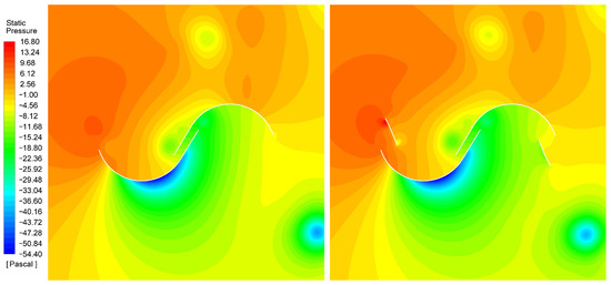
Figure 24.
Pressure contour graphs for the split Bach profile (left) and the multi-blade Bach profile (right) at a rotor azimuth angle () of 185° and a of 1.0996.
In the same way, an area of higher pressure can be evidenced on the secondary element of the opposite blade, which promotes the superior performance of the multi-element rotor in the following positions, by diverting a part of the flow toward the concavity of the main element (Figure 25).
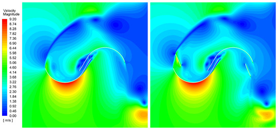
Figure 25.
Velocity contour graphs for the split Bach profile (left) and the multi-blade Bach profile (right) at a rotor azimuth angle () of 185° and a of 1.0996.
4.2. Manufacturing Feasibility
The multi-element geometry of the developed wind rotor largely preserves the constructive and operational simplicity that characterizes the Savonius type rotor. As can be seen in Figure 8, the plates installed at the ends of the rotor allow the assembly of secondary elements without requiring substantial modifications.
In the same way, every element that constitute the blade can be made of the same material. The additional material involved in the manufacture of the secondary elements represents only 21% of the material required by the main elements.
One of the main constructive advantages that is conserved in this new rotor is the possibility of manufacturing the blades from sheets of any material suitable for operating conditions, and which, keeping the required thickness, allow them to be shaped according to the geometry.
5. Conclusions
In this research, the optimal proportions of the secondary element of a multi-element geometry in a Savonius rotor with a split Bach type blade profile without an intermediate shaft wer numerically determined. The results showed that every factor analyzed had a statistically significant effect on the power coefficient in the experimental domain studied. Likewise, it was observed that there is a great interaction between the factors that determine the distance between the elements of the blade. The optimal dimensions obtained for said profile are 96.81, 17.43, and 9.4 in percentage values of the rotor diameter, for the parameters O, P, and Q, respectively.
Although the full factorial experimental design had greater acceptance within the purposes of this research, the face-centered central composite design allowed the rotor performance to be modeled with great adjustment, saving a third of the number of treatments.
The conventional semicircular profile rotor established as a reference, presented a of 0.195 in a flow close to a Reynolds number of and a blockage ratio of 2%. Likewise, the geometry with the split Bach type profile without secondary elements allows reaching a of 0.2661. In turn, the rotor with the multi-element profile optimized using the response surface methodology presented a of 0.2948, under the same conditions, which represents an increase of 51.2% and 10.8% in performance, respectively.
It was determined that the secondary element favors the performance during much of the advancing phase of the blade, when it receives the flow directly. In the last part of this phase and in the first half of the returning phase, a loss in performance is generated mainly due to the greater resistance that the additional surface implies. During the second half of the returning phase, there are no significant differences, which may be due to a slight increase in performance that allows to counteract the additional resistance.
Likewise, the rotors with conventional semicircular, split Bach, and multi-blade Bach profiles were experimentally studied using a wind tunnel under the same conditions established in the simulations. The numerical results used for verification were obtained from the simulation of computational replicas from the experimental setup of each rotor, considering the three-dimensionality and the degrees of freedom of the system. The difference between the results of the multi-blade Bach profile and the split Bach profile was found to be approximately half the difference between the latter and the conventional semicircular profile, both in the numerical and experimental approach.
Author Contributions
Conceptualization, L.A.G.; methodology, L.A.G. and F.A.O.; software, L.A.G. and F.A.O.; investigation, L.A.G.; resources, F.A.O.; data curation, E.L.C. and E.G.F.; writing—original draft preparation, L.A.G.; writing—review and editing, L.A.G., E.L.C. and E.G.F.; supervision, E.L.C. and E.G.F.; project administration, E.G.F. All authors have read and agreed to the published version of the manuscript.
Funding
This research received no external funding.
Acknowledgments
The authors gratefully acknowledge the financial support provided by the Colombia Scientific Program within the framework of the call Ecosistema Científico (Contract number FP44842-218-2018).
Conflicts of Interest
The authors declare no conflict of interest.
Abbreviations
The following abbreviations are used in this manuscript:
| FFD | full factorial experimental design |
| FCCD | face-centered central composite design |
| TSR | tip speed ratio |
| PWM | pulse width modulation |
| MAMSL | meters above mean sea Level |
| 6-DOF | six degrees of freedom |
References
- Mohammed, A.A.; Ouakad, H.M.; Sahin, A.Z.; Bahaidarah, H. Vertical axis wind turbine aerodynamics: Summary and review of momentum models. J. Energy Resour. Technol. 2019, 141. [Google Scholar] [CrossRef]
- Eriksson, S.; Bernhoff, H.; Leijon, M. Evaluation of different turbine concepts for wind power. Renew. Sustain. Energy Rev. 2008, 12, 1419–1434. [Google Scholar] [CrossRef]
- Zhang, B.; Song, B.; Mao, Z.; Tian, W. A novel wake energy reuse method to optimize the layout for Savonius type vertical axis wind turbines. Energy 2017, 121, 341–355. [Google Scholar] [CrossRef] [Green Version]
- Hansen, J.T.; Mahak, M.; Tzanakis, I. Numerical modelling and optimization of vertical axis wind turbine pairs: A scale up approach. Renew. Energy 2021, 171, 1371–1381. [Google Scholar] [CrossRef]
- Savonius, S.J. The S-rotor and its applications. Mech. Eng. 1931, 53, 333–338. [Google Scholar]
- Chen, L.; Chen, J.; Zhang, Z. Review of the Savonius rotor’s blade profile and its performance. J. Renew. Sustain. Energy 2018, 10, 013306. [Google Scholar] [CrossRef]
- Golecha, K.; Kamoji, M.; Kedare, S.; Prabhu, S. Review on Savonius rotor for harnessing wind energy. Wind Eng. 2012, 36, 605–645. [Google Scholar] [CrossRef]
- Kumar, A.; Saini, R. Performance parameters of Savonius type hydrokinetic turbine-A Review. Renew. Sustain. Energy Rev. 2016, 64, 289–310. [Google Scholar] [CrossRef]
- Al-Kayiem, H.H.; Bhayo, B.A.; Assadi, M. Comparative critique on the design parameters and their effect on the performance of S-rotors. Renew. Energy 2016, 99, 1306–1317. [Google Scholar] [CrossRef]
- Altan, B.D.; Atılgan, M. An experimental and numerical study on the improvement of the performance of Savonius wind rotor. Energy Convers. Manag. 2008, 49, 3425–3432. [Google Scholar] [CrossRef]
- Hu, Y.; Tong, Z.; Wang, S. A new type of VAWT and blade optimization. In Proceedings of the International Technology and Innovation Conference 2009 (ITIC 2009), Xi’an, China, 12–14 October 2009; pp. 1–5. [Google Scholar] [CrossRef]
- Shaughnessy, B.; Probert, S. Partially-blocked Savonius rotor. Appl. Energy 1992, 43, 239–249. [Google Scholar] [CrossRef]
- Shikha.; Bhatti, T.; Kothari, D. Vertical axis wind rotor with concentration by convergent nozzles. Wind Eng. 2003, 27, 555–959. [Google Scholar] [CrossRef]
- Mohamed, M.; Janiga, G.; Pap, E.; Thévenin, D. Optimization of Savonius turbines using an obstacle shielding the returning blade. Renew. Energy 2010, 35, 2618–2626. [Google Scholar] [CrossRef]
- Maldar, N.R.; Ng, C.Y.; Oguz, E. A review of the optimization studies for Savonius turbine considering hydrokinetic applications. Energy Convers. Manag. 2020, 226, 113495. [Google Scholar] [CrossRef]
- Alom, N.; Borah, B.; Saha, U.K. An insight into the drag and lift characteristics of modified Bach and Benesh profiles of Savonius rotor. Energy Procedia 2018, 144, 50–56. [Google Scholar] [CrossRef]
- Roy, S.; Saha, U.K. Review of experimental investigations into the design, performance and optimization of the Savonius rotor. Proc. Inst. Mech. Eng. Part A J. Power Energy 2013, 227, 528–542. [Google Scholar] [CrossRef]
- Schlichting, H.; Gersten, K. Boundary-Layer Theory; Springer: Berlin/Heidelberg, Germany, 2017. [Google Scholar] [CrossRef]
- Anderson, J.D., Jr. Fundamentals of Aerodynamics; Tata McGraw Hill Education: New York, NY, USA, 2017. [Google Scholar]
- Bertin, J.J.; Smith, M.L. Aerodynamics for Engineers; Prentice Hall: Upper Saddle River, NJ, USA, 1998; Volume 5. [Google Scholar]
- Cengel, Y.A.; Cimbala, J.M. Fluid Mechanics: Fundamentals and Applications, Forth Edition; Tata McGraw Hill Education: New York, NY, USA, 2018. [Google Scholar]
- Fox, R.W.; McDonald, A.T.; Mitchell, J.W. Fox and McDonald’s Introduction to Fluid Mechanics; John Wiley & Sons: Hoboken, NJ, USA, 2020. [Google Scholar]
- Clancy, L.J. Aerodynamics; John Wiley & Sons: Hoboken, NJ, USA, 1975. [Google Scholar] [CrossRef]
- White, F. Fluid Mechanics; Tata McGraw Hill Education: New York, NY, USA, 2011. [Google Scholar]
- Bah, E.A.; Sankar, L.N.; Jagoda, J.I. Numerical investigations on the use of multi-element airfoils for vertical axis wind turbine configurations. In Proceedings of the ASME 2013 Gas Turbine India Conference, Bangalore, India, 5–6 December 2013; American Society of Mechanical Engineers Digital Collection: New York, NY, USA, 2013. [Google Scholar] [CrossRef]
- Zhu, H.; Hao, W.; Li, C.; Ding, Q. Effect of flow-deflecting-gap blade on aerodynamic characteristic of vertical axis wind turbines. Renew. Energy 2020, 158, 370–387. [Google Scholar] [CrossRef]
- Atalay, K.D.; Dengiz, B.; Yavuz, T.; Koç, E.; İç, Y.T. Airfoil-slat arrangement model design for wind turbines in fuzzy environment. Neural Comput. Appl. 2020, 32, 13931–13939. [Google Scholar] [CrossRef]
- Roy, S.; Saha, U.K. Wind tunnel experiments of a newly developed two-bladed Savonius-style wind turbine. Appl. Energy 2015, 137, 117–125. [Google Scholar] [CrossRef]
- Montgomery, D.C. Design and Analysis of Experiments; John Wiley & Sons: Hoboken, NJ, USA, 2017. [Google Scholar]
- Mathew, S. Wind Energy: Fundamentals, Resource Analysis and Economics; Springer: Berlin/Heidelberg, Germany, 2006. [Google Scholar] [CrossRef]
- Abraham, J.; Mowry, G.; Plourde, B.; Sparrow, E.; Minkowycz, W. Numerical simulation of fluid flow around a vertical-axis turbine. J. Renew. Sustain. Energy 2011, 3, 033109. [Google Scholar] [CrossRef]
- Andersson, B.; Andersson, R.; Haakansson, L.; Mortensen, M.; Sudiyo, R.; Van Wachem, B. Computational Fluid Dynamics for Engineers; Cambridge University Press: Cambridge, UK, 2011. [Google Scholar]
- Menter, F.R.; Kuntz, M.; Langtry, R. Ten years of industrial experience with the SST turbulence model. Turbul. Heat Mass Transf. 2003, 4, 625–632. [Google Scholar]
- Alom, N.; Saha, U.K. Influence of blade profiles on Savonius rotor performance: Numerical simulation and experimental validation. Energy Convers. Manag. 2019, 186, 267–277. [Google Scholar] [CrossRef]
- Jain, P. Wind Energy Engineering; McGraw Hill: New York, NY, USA, 2011. [Google Scholar]
- Versteeg, H.K.; Malalasekera, W. An Introduction to Computational Fluid Dynamics: The Finite Volume Method; Pearson Education: Harlow, Essex, UK, 2007. [Google Scholar]
- Ross, I.; Altman, A. Wind tunnel blockage corrections: Review and application to Savonius vertical-axis wind turbines. J. Wind Eng. Ind. Aerodyn. 2011, 99, 523–538. [Google Scholar] [CrossRef]
- Roy, S.; Saha, U.K. An adapted blockage factor correlation approach in wind tunnel experiments of a Savonius-style wind turbine. Energy Convers. Manag. 2014, 86, 418–427. [Google Scholar] [CrossRef]
- Almohammadi, K.; Ingham, D.; Ma, L.; Pourkashan, M. Computational fluid dynamics (CFD) mesh independency techniques for a straight blade vertical axis wind turbine. Energy 2013, 58, 483–493. [Google Scholar] [CrossRef]
- Alom, N.; Saha, U.K. Arriving at the optimum overlap ratio for an elliptical-bladed Savonius rotor. In Turbo Expo: Power for Land, Sea, and Air; American Society of Mechanical Engineers: New York, NY, USA, 2017; Volume 50961, p. V009T49A012. [Google Scholar] [CrossRef]
- Jeon, K.S.; Jeong, J.I.; Pan, J.K.; Ryu, K.W. Effects of end plates with various shapes and sizes on helical Savonius wind turbines. Renew. Energy 2015, 79, 167–176. [Google Scholar] [CrossRef]
- Mason, R.L.; Gunst, R.F.; Hess, J.L. Statistical Design and Analysis of Experiments: With Applications to Engineering and Science; John Wiley & Sons: Hoboken, NJ, USA, 2003; Volume 474. [Google Scholar]
- Myers, R.H.; Montgomery, D.C.; Anderson-Cook, C.M. Response Surface Methodology: Process and Product Optimization Using Designed Experiments; John Wiley & Sons: Hoboken, NJ, USA, 2016. [Google Scholar]
- Van Rooij, R.; Timmer, W. Roughness sensitivity considerations for thick rotor blade airfoils. J. Sol. Energy Eng. 2003, 125, 468–478. [Google Scholar] [CrossRef]


Publisher’s Note: MDPI stays neutral with regard to jurisdictional claims in published maps and institutional affiliations. |
© 2021 by the authors. Licensee MDPI, Basel, Switzerland. This article is an open access article distributed under the terms and conditions of the Creative Commons Attribution (CC BY) license (https://creativecommons.org/licenses/by/4.0/).