Hierarchical Active Tracking Control for UAVs via Deep Reinforcement Learning

Abstract

Active tracking control is essential for UAVs to perform autonomous operations in GPS-denied environments. In the active tracking task, UAVs take high-dimensional raw images as input and execute motor actions to actively follow the dynamic target. Most research focuses on three-stage methods, which entail perception first, followed by high-level decision-making based on extracted spatial information of the dynamic target, and then UAV movement control, using a low-level dynamic controller. Perception methods based on deep neural networks are powerful but require considerable effort for manual ground truth labeling. Instead, we unify the perception and decision-making stages using a high-level controller and then leverage deep reinforcement learning to learn the mapping from raw images to the high-level action commands in the V-REP-based environment, where simulation data are infinite and inexpensive. This end-to-end method also has the advantages of a small parameter size and reduced effort requirements for parameter turning in the decision-making stage. The high-level controller, which has a novel architecture, explicitly encodes the spatial and temporal features of the dynamic target. Auxiliary segmentation and motion-in-depth losses are introduced to generate denser training signals for the high-level controller’s fast and stable training. The high-level controller and a conventional low-level PID controller constitute our hierarchical active tracking control framework for the UAVs’ active tracking task. Simulation experiments show that our controller trained with several augmentation techniques sufficiently generalizes dynamic targets with random appearances and velocities, and achieves significantly better performance, compared with three-stage methods.

1. Introduction

Unmanned aerial vehicles (UAVs) are becoming an ideal platform to execute dirty and dangerous tasks, due to their high agility and low cost. Perception and control are the two key modules of autonomous UAVs. Without these, UAVs cannot derive rich information from the complex environment, make proper decisions and behave correctly. Autonomous perception and smart control are always topics of interest in the UAV community.

In this paper, we focus on the active tracking task of UAVs. Active tracking for a dynamic target is a fundamental function for UAVs to perform monitoring and anti-terrorism operations in GPS-denied environments. This specific task requires both autonomous perception to determine the location of the dynamic target and control to actively track the target, which can be transferred and generalized to more difficult autonomous tasks.

Most research considers the active tracking task to be three separate subproblems, namely, perceive first, make movement decisions based on the target’s estimated position, and then control the UAV dynamics [1,2,3,4]. In the perception stage, early research used traditional computational vision techniques, such as filtering in HSV space and the Hough transform, to detect objects with certain colors or shapes. Later research used hand-crafted features, such as SIFT [5] and SURF [6], to detect more random objects. Recent research combines a convolutional neural network (CNN)–based object detector [7,8,9,10] and a passive tracker [11,12,13,14,15] to obtain the bounding box of the target of interest. In the decision-making stage, control methods, such as proportional integral derivative (PID), calculate high-level action commands based on the coordinates of the bounding box’s center and relative changes in the bounding box’s height. PID is also usually used to control UAVs’ low-level dynamics. However, training the CNN-based visual perception module requires considerable effort for ground truth labeling, and the parameter tuning process for the high-level decision-making module may cause unexpected damage to UAVs.

Reinforcement learning (RL) holds promise for automated learning perception and control simultaneously. RL has several applications in the UAV community. Omar et al. used RL to learn an aggressive trajectory tracking controller for UAVs [16]. Manan et al. applied RL to teach UAV vision-based guidance tasks [17]. Riccardo et al. achieved autonomous landing on the deck of an unmanned surface vehicle, using RL [18]. Through trial and error, model-free deep RL can learn complicated high-level control policies for UAVs, which maps visual observations to action commands directly. This end-to-end solution trains perception and control concurrently for UAVs’ active tracking task in the virtual environment and overcomes the problems encountered by three-stage methods. Luo et al. [19] used the ConvNet-LSTM network as the high-level policy network, which performs well in different active tracking scenarios but does not focus on the UAV domain and cannot transfer directly without considering the dynamic properties of the UAV. Li et al. [20] proposed a hierarchical control system that uses the policy network trained by deep RL as the high-level decision-making layer and the PID controller as the low-level command execution layer. However, the system does not consider the speed of the dynamic target and the action space, and a relative position offset may cause volatile behaviors that cannot be precisely tracked by the PID controller. Moreover, additional features (quadrotor altitude, linear velocity, orientation, and angular velocity) must be included as a part of the decision-making layer input to achieve stable flight. In this paper, we propose a novel hierarchical control framework for UAVs’ active tracking task. This framework uses the neural-based end-to-end perception and decision-making method for the high-level control module and the traditional control method for the low-level control module. Unlike the above methods that do not consider the UAV dynamics and target speed, all these factors are taken into account in this framework. The main contributions of this paper are summarized as follows:

• We develop a novel and interpretable neural architecture for the high-level controller to derive the spatial and temporal latent features of the dynamic target and output continuous tracking speed commands directly. This compact architecture reduces the number of parameters of the high-level controller.
• End-to-end mapping from raw images to the high-level decision is trained via deep RL in the virtual environment based on V-REP [21]. We also leverage PyRep [22] to accelerate the simulation speed and run parallel environments for faster data collection. The simulation data are inexpensive, and no effort for ground-truth labeling is needed.
• To further accelerate the training process, we adopt auxiliary segmentation and motion-in-depth losses, which can generate denser training signals.
• Augmentation techniques are applied in the virtual environment to increase the robustness of the trained controller.

In our experiment, the proposed hierarchical control framework and auxiliary losses can effectively decrease the training time. The quadrotor with a trained high-level control module and low-level PID control module can adapt to the dynamic target with random colors, paths, and speeds in the UAVs’ active tracking task.

2. Preliminary Considerations

2.1. Markov Decision Process

In the RL problem, the interaction process between the agent and the environment is usually modeled as a Markov decision process (MDP) [23]. The MDP can be denoted as $M=(S,A,P,{\rho }_0,r,\gamma )$, where S is the state space, A is the action space, $P(S_{t+1}=s^{\prime }\mid S_t=s,A_t=a):S\times A\times S\to [0,1]$ is the probability of transitioning into state $s^{\prime }$ upon taking action a in state s, $r(s,a):S\times A\to \mathbb{R}$ is the immediate reward associated with taking action a in state s, $\gamma \in [0,1)$ is the discount factor and defines the horizon of the RL problem, and ${\rho }_0:S\to [0,1]$ is the initial state distribution.

Given the MDP M and a parameterized policy ${\pi }_{\theta }:S\to A$, the agent interacts with the environment following the trajectory $\tau$:

$$\tau =(s_0,a_0,r_1,s_1,\cdots ,s_T)$$

(1)

where $s_0\sim {\rho }_0,s_t\sim P\left(·\mid s_{t-1},a_{t-1}\right),a_t\sim {\pi }_{\theta }\left(·\mid s_t\right),r_t=r\left(s_t,a_t\right)$ and T is the horizon length.

The goal of the deep RL problem is to identify an optimal policy ${\pi }_{\theta }^{*}$ that maximizes the expected discounted return:

$$J={\mathbb{E}}_{\tau }\left[\sum _{t=0}^{T-1}{\gamma }^t{r}_t\right]$$

(2)

2.2. Proximal Policy Optimization Algorithm

Policy gradient methods in RL are sensitive to hyperparameters, such as the policy update step. If the policy is updated in an unfavorable direction, the policy will be worse when using the sampled experiences in the next update iteration.

Trust region policy optimization (TRPO) [24] avoids significant and destructive policy parameter changes with a KL divergence constraint $\delta$ on the size of the policy update at each iteration:

$$\begin{array}{cc}\underset{\theta }{maximize}\hfill & {\widehat{\mathbb{E}}}_t\left[\frac{{\pi }_{\theta }\left(a_t\mid s_t\right)}{{\pi }_{{\theta }_{\mathrm{old}}}\left(a_t\mid s_t\right)}{\widehat{A}}_t\right]\hfill \\ \mathrm{subject}\mathrm{to}\hfill & {\widehat{\mathbb{E}}}_t\left[KL\left[{\pi }_{{\theta }_{\mathrm{old}}}\left(·\mid s_t\right),{\pi }_{\theta }\left(·\mid s_t\right)\right]\right]\le \delta \hfill \end{array}$$

(3)

where ${\widehat{A}}_t$ is an estimator of the advantage function at timestep t and ${\theta }_{old}$ represents the parameters of the policy before the update. TRPO approximates Equation (3) by linear objective and quadratic constraints and then solves it with the conjugate gradient algorithm.

Schulman et al. [25] proposed the proximal policy optimization (PPO) algorithm to further simplify TRPO.

PPO denotes the probability ratio as $r_t\left(\theta \right)$:

$$r_t\left(\theta \right)=\frac{{\pi }_{\theta }(a_t\mid s_t)}{{\pi }_{{\theta }_{old}}(a_t\mid s_t)}$$

(4)

and proposes a new objective as follows:

$$\begin{array}{cc}{\mathcal{L}}^{\mathrm{Clip}}\left(\theta \right)\hfill & ={\widehat{\mathbb{E}}}_t\left[min\left(r_t\left(\theta \right)5{\widehat{A}}_t,{clip}_{obj}\right)\right]\hfill \\ {clip}_{obj}\hfill & =clip\left(r_t\left(\theta \right),1-ϵ,1+ϵ\right){\widehat{A}}_t\hfill \end{array}$$

(5)

where $ϵ$ is a hyperparameter that clips the moving $r_t$ in the range $[1-ϵ,1+ϵ]$.

The minimum of the clipped objective ${clip}_{obj}$ is taken as the final objective, which restricts large policy updates. PPO has been demonstrated to work well on a collection of benchmark tasks, including simulated robotic locomotion and Atari game playing [25], and is one of the most powerful model-free deep RL algorithms.

2.3. Generalized Advantage Estimation

To reduce variance in policy gradient methods, Schulman et al. [26] proposed the generalized advantage estimator (GAE) as follows:

$$\begin{array}{cc}\hfill {\widehat{A}}_t^{GAE(\gamma ,\lambda )}& =\sum _{l=1}^{\infty }{\left(\gamma \lambda \right)}^l{\delta }_{t+l}^V\hfill \\ \hfill & =\sum _{l=1}^{\infty }{\left(\gamma \lambda \right)}^l\left(r_t+\gamma V\left(s_{t+l+1}\right)-V\left(s_{t+l}\right)\right)\hfill \end{array}$$

(6)

GAE is a general form of the following two advantage estimators:

$${\widehat{A}}_t:={\delta }_t=r_t+\gamma V\left(s_{t+1}\right)-V\left(s_t\right)$$

(7)

$${\widehat{A}}_t:=\sum _{l=0}^{\infty }{\gamma }^l{\delta }_{t+l}=\sum _{l=0}^{\infty }{\gamma }^l{r}_{t+l}-V\left(s_t\right)$$

(8)

Equation (7) is biased but has low variance, while Equation (8) is unbiased but has high variance, due to the sum of many terms. GAE unifies these two advantage estimators and balances between the bias and the variance for advantage estimation by parameter $\lambda \in (0,1)$. Equations (7) and (8) are the specific cases of Equation (6) when $\lambda =0$ and $\lambda =1$, respectively.

3. Methodology

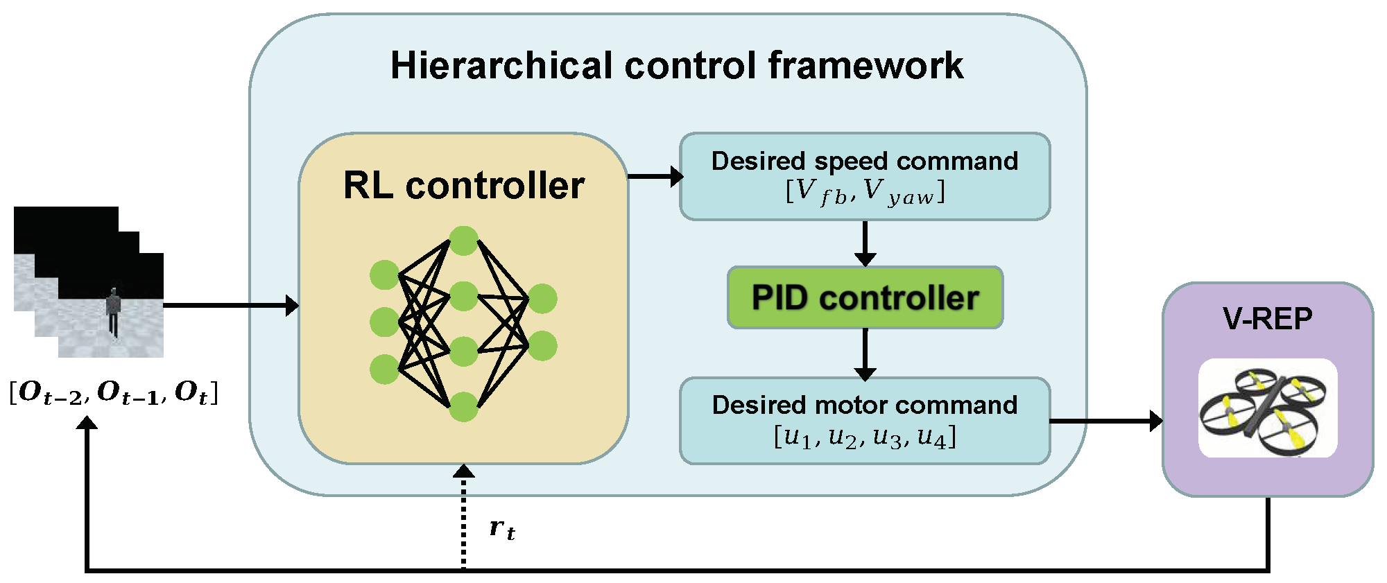
3.1. Hierarchical Control Framework

In the active tracking task, quadrotors use only the raw images captured by the onboard camera to execute proper subsequent actions. Since the raw images are very high-dimensional observations, designing an effective controller for quadrotors manually is challenging. Instead, we build a neural network controller and train it via deep RL. In theory, this learning method can map raw images to quadrotor motor commands directly. However, the deep RL method suffers from the problems of exploration and local optimality. Training such a complicated policy is not easy, even with sufficient interaction data between the quadrotor and the environment.

We propose a hierarchical controller framework, as shown in Figure 1, to solve this dilemma. This framework consists of two-level policy layers. In the high-level policy layer, the neural RL controller outputs the desired speed commands for the quadrotor, given three sequential raw images $[{\mathbf{O}}_{t-2},{\mathbf{O}}_{t-1},{\mathbf{O}}_t]$ as inputs. This high-level RL controller perceives the features of the dynamic target and makes high-level decisions to follow it. The high-level decisions consist of the desired linear speed along the head direction $V_{fb}$ and the desired yaw speed $V_{yaw}$. In the low-level policy layer, the PID controller is used to track high-level decisions under the current altitude and speed and then outputs the desired motor commands $[u_1,u_2,u_3,u_4]$ for the quadrotor. This hierarchical framework enables us to focus on the learning of a high-level RL controller without concern for the low-level dynamic control of the quadrotor.

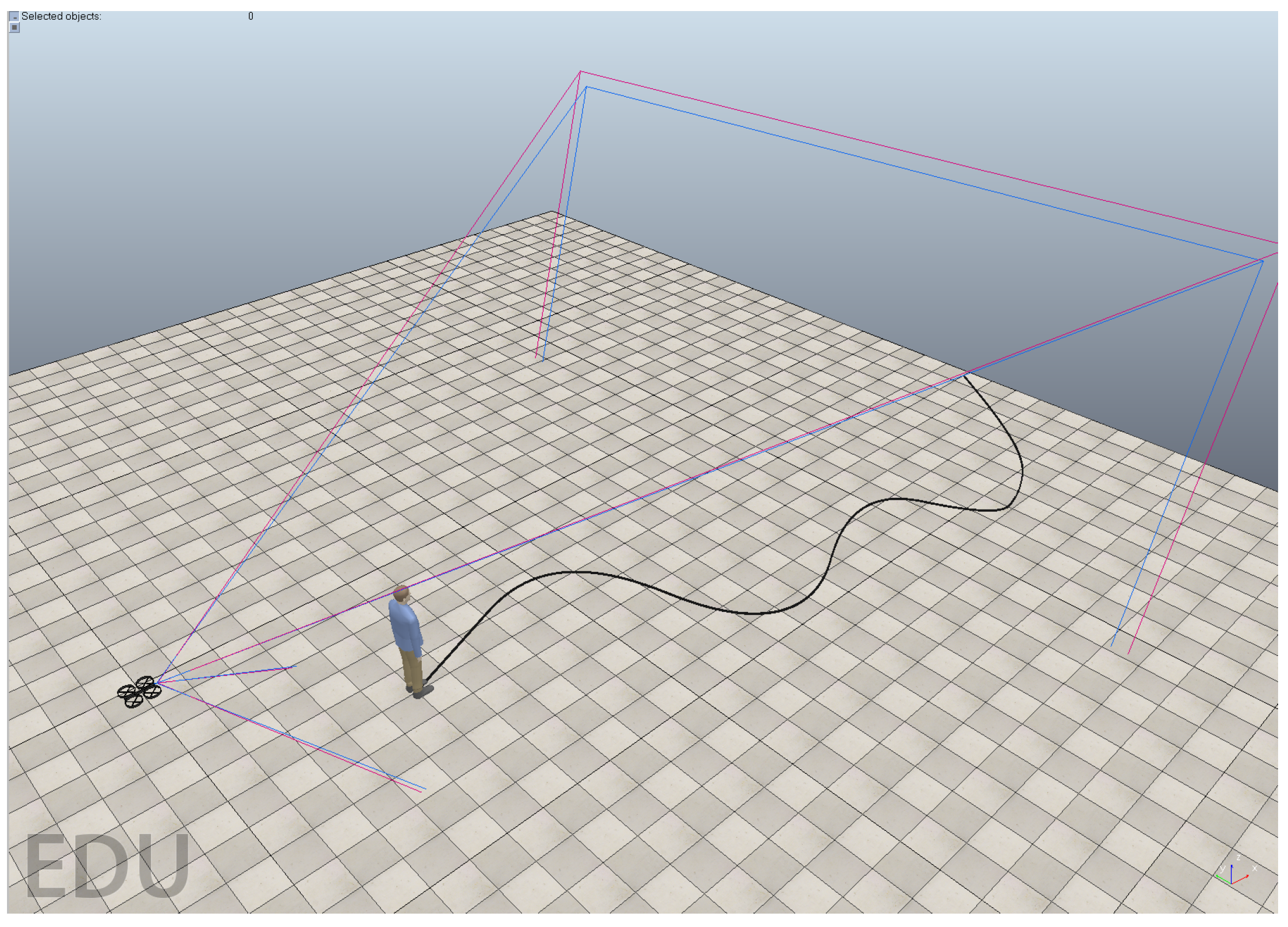
3.2. Simulator Set-Up and Augmentation

Due to the data inefficiency issue of model-free RL, extensive interaction data with the environment are necessary to improve the high-level RL controller through trial and error. We cannot afford to train our RL controller for quadrotors in the real world. Instead, we set up a simulation environment where the quadrotors can gain infinite and high-fidelity training data.

Based on the virtual robot experimentation platform (V-REP) [21], we build an RL training environment for the quadrotor’s active tracking task, as shown in Figure 2. In this environment, three main entities exist: a quadrotor equipped with a camera, an IMU and an altitude ranging sensor, and a dynamic person (the target) walking along a path from the beginning to the end. The camera is tilted down 30 degrees relative to the horizontal plane. The quadrotor uses sequential images from the camera as the observation and decides the desired speed commands using the RL controller to follow the dynamic target. Then, the quadrotor uses the IMU and altitude ranging sensor to obtain the current velocity and height information and applies the desired motor commands to track the desired speed commands while maintaining its altitude via the PID controller. Next, the environment returns the reward function and the next observation. At the initialization of each training episode, the target people will be in front of the quadrotor.

To enhance the generalizability of our trained RL controller to various domains, we adopt several environmental augmentation methods as follows.

• Visual randomization: We divide the appearance of the target person into five parts—hair, skin, shirt, trousers, and shoes. Then, we change the color of each part at every timestep, which is helpful to learn the dynamic target’s more essential features rather than simply memorizing the colors.
• Speed randomization: To learn an RL controller that is less sensitive to the target’s velocity, we change the walking speed of the target person at every timestep in the interval $[0,V_{target}]$ uniformly.
• Path randomization: To increase the robustness of the RL controller to the gestures and relative position of the target, we randomly sample n control points between the beginning and the end of the path and then generate a smooth trajectory using a B-spline for every training episode. The target person will follow the random trajectories under control.

The simulation speed is the main concern when training with data-driven model-free RL methods. However, the original Python remote API of V-REP is not sufficiently fast. To accelerate the training process, we leverage PyRep [22] to break this data generation bottleneck. PyRep is built on top of the V-REP and can provide a flexible API and significant acceleration. Moreover, the simulation environments are easy to parallelize, implying that several workers can be used to interact with different environments at the same time and accelerate the training even further.

3.3. RL Controller Architecture

The neural RL controller is an actor–critic style architecture, as shown in Figure 3. Given the sequential images $[{\mathbf{O}}_{t-2},{\mathbf{O}}_{t-1},{\mathbf{O}}_t]$ as observations, the actor network and the critic network share the perception layer, which consists of the spatial and temporal feature encoders. This shared perception layer is designed to extract the spatial and temporal features of the dynamic target. The rest of the actor network and the critic network calculate the continuous normalized desired speed commands $[{\overline{V}}_{fb},{\overline{V}}_{yaw}]$ and the estimated value of the observation, respectively.

This end-to-end perception and control method maps the high-dimensional raw images to the high-level actions directly. The mapping is learned via deep RL in the virtual environment, which saves the effort typically required for ground-truth labeling for perception learning and parameter tuning for simultaneous perception and control. The layers with a specific function improve the interpretability of the RL controller.

3.3.1. Attention-Based Spatial Feature Encoder

In the active tracking task, the quadrotor should first know the location of the dynamic target. To reduce the computational cost of the RL controller, a compact neural network architecture with powerful representational capacity is necessary. We leverage the convolutional block attention module (CBAM) [27], which consists of a 1D channel attention module and a 2D spatial attention module. The channel attention module focuses on ’what’ is meaningful in the input image, while the spatial attention module tends to know ’where’ informative parts are located. Given a raw image input, CBAM can help extract the spatial information of our dynamic target of interest.

3.3.2. Feature Difference-Based Temporal Feature Encoder

For better adaptation to the target’s different velocities, not only the spatial features, but also the temporal features of the dynamic target must be determined. A small optical flow network is used to incorporate explicit temporal information of the dynamic target in [28]. However, computing optical flow is still expensive, and we can encode the temporal information more efficiently. Unlike the latent flow method in [29], which fuses raw images and their differences directly, we focus on our target of interest and first extract the spatial features of three sequential raw images by the shared convolutional block attention module and then concatenate the spatial features and their differences. A 2D convolution layer processes these fused features further to extract the temporal information of the dynamic target.

3.3.3. Decision-Making and Value-Fitting Layer

The spatial and temporal feature encoders constitute the final perception layer, which encodes the spatial and temporal features of the dynamic target, followed by the standard RL actor–critic architecture. We adopt two fully connected (FC) layers for decision-making and value fitting. The value-fitting layer estimates the value function of the observation. The decision-making layer computes the mean of the continuous high-level actions ${\overrightarrow{\mu }}_a={[a_1,a_2]}^T$. In the training stage, the high-level actions are sampled from the following:

$${[{\widehat{V}}_{fb},{\widehat{V}}_{yaw}]}^T\sim {\overrightarrow{\mu }}_a+\mathcal{N}(\mathbf{0},\mathsf{\Sigma })$$

(9)

where $\mathsf{\Sigma }$ is the diagonal covariance matrix. The Gaussian noise is helpful for exploration.

Then, the high-level actions are clipped into the range to be normalized:

$$\begin{array}{cc}{\overline{V}}_{fb}\hfill & =clip({\widehat{V}}_{fb},-1,1)\hfill \\ {\overline{V}}_{yaw}\hfill & =clip({\widehat{V}}_{yaw},-1,1)\hfill \end{array}$$

(10)

The details of the RL controller’s network architecture are presented in Appendix A.

3.4. Reward Engineering

Figure 4 shows the aerial view and abstraction of the training environment. The y-axis is set to the head direction of the quadrotor, and the x-axis is set from the quadrotor’s right to left. The coordinate of the target in this quadrotor’s body frame is denoted as $(dx,dy)$; then, the yaw angle $\phi$ and distance $\rho$ between the target and quadrotor can be calculated as follows:

$$\begin{array}{cc}\phi \hfill & =arctan(dx/dy)\hfill \\ \rho \hfill & =\sqrt{{dx}^2+{dy}^2}\hfill \end{array}$$

(11)

We want the quadrotor to follow the target at a fixed distance ${\rho }_d$ while being oriented toward the target; thus, the following naive reward function is proposed, which encourages $\rho ={\rho }_d$ and $\phi =0$:

$$r={\alpha }_{1}exp(-\left|\frac{\rho -{\rho }_d}{{\beta }_1}\right|)+{\alpha }_{2}exp(-\left|\frac{\phi }{{\beta }_2}\right|)$$

(12)

where ${\alpha }_1>0,{\alpha }_2>0,{\beta }_1>0,{\beta }_2>0$ are tunable hyperparameters. ${\beta }_1,{\beta }_2$ control the gradient of the first and second parts of the exponential reward function, respectively, and ${\alpha }_1,{\alpha }_2$ are their coefficients of combination.

3.5. Auxiliary Segmentation and Motion-in-Depth Loss

While the RL controller’s architecture is designed to have a powerful spatial and temporal representational capacity, the RL controller is still difficult to properly train using the model-free RL method since the input state is so highly dimensional; this training process is very data inefficient. Moreover, the perception layer in the RL controller may not learn the correct spatial and temporal features of the dynamic target guided by such a highly abstract reward signal.

To accelerate the training process and build a good representation of the perception layer in the RL controller, supervised learning is combined with the RL method. Additionally, two auxiliary losses are added in the training process, namely, the segmentation loss and the motion-in-depth loss. Then, supervised learning assists the RL training process by training additional auxiliary losses. The auxiliary losses introduced can generate denser signals that facilitate the learning of spatial and temporal representations.

3.5.1. Auxiliary Segmentation Loss

In the spatial features encoder, the output latent features are supposed to represent the spatial information of the dynamic target in our design. To provide denser training signals, we add the auxiliary segmentation loss after the convolutional block attention module, as shown in Figure 3.

The output map of the convolutional block attention module is denoted as ${\mathbf{Z}}_n$, and the ground-truth segmentation map is denoted as ${\mathbf{G}}_n$ given input ${\mathbf{O}}_n$, where ${\mathbf{Z}}_n$ is followed by the sigmoid activation function $\sigma$ to predict the probability map ${\mathbf{P}}_n$ for each pixel in ${\mathbf{Z}}_n$:

$$p_{ij}^n=\sigma \left(z_{i,j}\right)=\frac{1}{1+exp(-z_{i,j})}\mathrm{for}(i,j)\in {\mathbf{Z}}_n$$

(13)

Then, the auxiliary segmentation loss is the binary cross-entropy between the predicted probability $p_{i,j}^n$ and ground truth $g_{i,j}^n$ for each pixel in ${\mathbf{Z}}_n$:

$$\begin{array}{cc}\hfill {\mathcal{L}}^{\mathrm{Seg}}=& -\sum _{n=t-2}^t\frac{1}{|{\mathbf{P}}_n|}\hfill \\ \hfill & \sum _{(i,j)\in {\mathbf{P}}_n}{g}_{ij}^{n}log{p}_{ij}^n+\left(1-g_{ij}^n\right)log\left(1-p_{ij}^n\right)\hfill \end{array}$$

(14)

where $g_{i,j}^n\in \{0,1\}$, and 1 corresponds to the target class, while 0 corresponds to the background class.

3.5.2. Auxiliary Motion-in-Depth Loss

The temporal feature encoder in the RL controller is designed to encode the temporal information of the dynamic target. The temporal information should contain the change in the dynamic target’s position that is parallel to the quadrotor’s camera view plane and the relative depth change of the dynamic target that is vertical to the quadrotor’s camera view plane. Among these, the depth change feature is more difficult to extract since the input resolution is set to be small for faster training, and the occupied resolution of the dynamic target is even smaller. To learn the dynamic target’s position change vertical to the quadrotor’s camera view plane, we need to introduce some auxiliary training signals at the end of the velocity perception layer.

For a dynamic target, suppose that the length projected on the image plane and the depth from the camera center at timestep t are $l_t$ and $d_t$, respectively. We can denote the optical expansion s between two timesteps as $t_i,t_j$, which indicates the relative scale change of the dynamic target as follows:

$$s_i^j=\frac{l_j}{l_i}$$

(15)

We can also denote the motion-in-depth $\tau$ between two timesteps $t_i,t_j$, which indicates the relative depth change of the dynamic target as follows:

$${\tau }_i^j=\frac{d_j}{d_i}$$

(16)

Interestingly, the motion-in-depth is the reciprocal of the optical expansion [30], indicating that they are unified and can both represent the vertical position change information of the dynamic target. Because the motion-in-depth is easier to calculate, we choose to adopt auxiliary motion-in-depth loss as the additional training signal for the velocity perception layer, as shown in Figure 3.

In [30], the motion-in-depth $\tau$ is calculated as the ratio between the depth of corresponding points over two frames as follows:

$${\tau }_i^j=\frac{d\left({\mathbf{x}}_{\mathbf{j}}\right)}{d\left({\mathbf{x}}_{\mathbf{i}}\right)}$$

(17)

where ${\mathbf{x}}_{\mathbf{i}}$ represents the occupied pixels of the dynamic target at the first frame and ${\mathbf{x}}_{\mathbf{j}}$ represents the correspondence of ${\mathbf{x}}_{\mathbf{i}}$ at the second frame.

We further simplify the calculation of motion-in-depth by ignoring the pixel matching over two frames for fast training:

$${\widehat{\tau }}_i^j=\frac{d\left({\mathbf{y}}_{\mathbf{j}}\right)}{mind\left({\mathbf{y}}_{\mathbf{i}}\right)}$$

(18)

where ${\mathbf{y}}_{\mathbf{i}}$ and ${\mathbf{y}}_{\mathbf{j}}$ are the occupied pixels of the dynamic target over two frames at timesteps $t_i$ and $t_j$, respectively. Due to the condition for training episode termination in our setting (listed in Section 4.1.1), the dynamic target is always in view of the quadrotor at training time, and $\left[d\left({\mathbf{y}}_{\mathbf{j}}\right),d\left({\mathbf{y}}_{\mathbf{i}}\right)\right]$ can be obtained directly in V-REP; thus, ${\widehat{\tau }}_i^j$ is always available during training.

The output map of the velocity perception layer is denoted as $\mathbf{W}$, and the motion-in-depth map over timestep $t-2$ and t is denoted as ${\widehat{\tau }}_{t-2}^t$. We resize ${\widehat{\tau }}_{t-2}^t$ as $\mathbf{M}$ to be the same size as $\mathbf{W}$ and then calculate the auxiliary motion-in-depth loss as follows:

$${\mathcal{L}}^{\mathrm{Dep}}=\frac{1}{\left|\mathbf{W}\right|}\sum _{(i,j)\in \mathbf{W}}{∥log{m}_{i,j}-w_{ij}∥}_2^2$$

(19)

where $m_{i,j}$ and $w_{i,j}$ are the pixels of $\mathbf{M}$ and $\mathbf{W}$, respectively.

Note that we skip frame $t-1$ because the motion-in-depth over two contiguous frames can be too small to guide the learning process effectively.

With both auxiliary segmentation and motion-in-depth losses, the total loss for the updating policy is the following:

$${\mathcal{L}}^{\mathrm{Total}}={\mathcal{L}}^{\mathrm{CLip}}+C_{Seg}{\mathcal{L}}^{\mathrm{Seg}}+C_{Dep}{\mathcal{L}}^{\mathrm{Dep}}$$

(20)

where $C_{Seg}>0$ and $C_{Dep}>0$ are tunable hyperparameters.

4. Experiments

4.1. Training

4.1.1. Environment Settings

The V-REP-based simulator is set up for the active tracking task. The observed state of the quadrotor is three sequential raw images $s_t=\left[{\mathbf{O}}_{t-2},{\mathbf{O}}_{t-1},{\mathbf{O}}_t\right]$ with a resolution of 64 × 64. Given the observed state $s_t$, the RL controller outputs the normalized desired speed commands, which consist of the linear velocity along with the head direction ${\overline{V}}_{fb}\in \left[-1,1\right]$ m/s and the yaw speed ${\overline{V}}_{yaw}\in \left[-1,1\right]$ rad/s. Then, the normalized desired speed commands are scaled to the final desired speed commands:

$$\begin{array}{cc}\hfill V_{fb}& =C_{fb}{\overline{V}}_{fb}\hfill \\ \hfill V_{yaw}& =C_{yaw}{\overline{V}}_{yaw}\hfill \end{array}$$

(21)

where the scales $C_{fb}$ and $C_{yaw}$ are set to be 0.8 and 0.1, respectively.

The final desired speed commands are tracked by the PID controller while maintaining the altitude at 2 m. The desired distance between the quadrotor and the target ${\rho }_d$ is 3 m.

At the start of each training episode, the quadrotor is 3 m behind the dynamic target (virtual person), and the dynamic target is in the center of the quadrotor’s view. The target’s end position is set to be 10 m away from the starting position. During the training, the visual, speed, and path randomization augmentation techniques in Section 3.2 are applied. The maximum speed of dynamic target $V_{target}$ is 0.5 m/s, and the number of sampled control points between the target’s start and end positions n is 8. When one of the following conditions is satisfied, the current training episode is completed, and the next training episode can begin:

• The dynamic target is out of the view of the quadrotor.
• The distance between the target and the quadrotor is out of the interval of [2, 4] m.
• The target reaches its end position.

4.1.2. Implementation Details

We use the model-free algorithm PPO with auxiliary losses to train our active tracking RL controller. The modified PPO algorithm is summarized in Algorithm 1. Adam [31] is used for optimization of the RL controller. The hyperparameters for the reward function, modified PPO algorithm, and optimizer are listed in

Table 1. Hyperparameters in our implementation.

Hyperparameter	Value
Number of actors N	2
Horizon T	2048
Adam stepsize	$5\times {10}^{-5}$
Num. epochs	2
Minibatch size	640
Discount $\gamma$	0.99
GAE parameter $\lambda$	0.98
Clipping $ϵ$	0.2
Auxiliary loss coefficient $C_{Seg}$	1.0
Auxiliary loss coefficient $C_{Dep}$	0.05
Reward coefficient ${\alpha }_1$	0.5
Reward coefficient ${\alpha }_2$	0.5
Reward coefficient ${\beta }_1$	0.5
Reward coefficient ${\beta }_2$	0.5

. Our algorithm is implemented by Pytorch [32].

Algorithm 1:PPO with auxiliary losses.

4.1.3. Ablation Studies in the Learning Process

We train our RL controller for the active tracking task through trial and error in the customized V-REP-based environment. We also perform ablation studies to evaluate the importance of the proposed auxiliary losses and the hierarchical control framework. Two groups of experiments are compared:

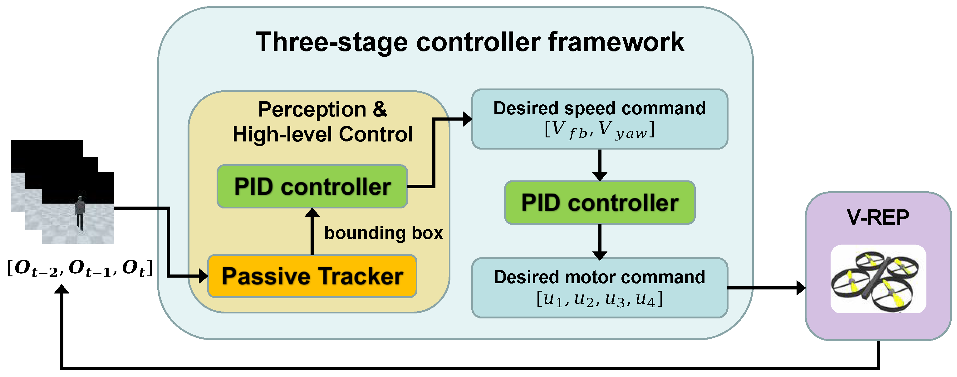
• The proposed hierarchical active tracking controller framework, which uses the RL controller for perception and high-level decision-making, and the PID controller is used for low-level dynamic control.
• The end-to-end active tracking controller framework, which maps raw image observations to a UAV’s motor commands directly.

In each group, four additional experiments are also compared:

• Training with auxiliary segmentation and motion-in-depth loss.
• Training with auxiliary segmentation but without motion-in-depth loss.
• Training without auxiliary segmentation but with motion-in-depth loss.
• Training without auxiliary segmentation and motion-in-depth loss.

The learning curves of all experiments are presented in Figure 5. All experiments in the end-to-end active tracking control learning group, as shown in Figure 5a, cannot achieve notable progress during the learning process, indicating that learning the direct mapping from high-dimensional observations to low-level motor commands is extremely complicated. With the hierarchical control framework, the learning of an active tracking controller is much more efficient, as presented in Figure 5b. We can observe that training with auxiliary segmentation and motion-in-depth loss can converge quickly and achieve good asymptotic performance. The performance of training with only one of the two auxiliary losses suffers from the problem of weak stability. Training without any auxiliary losses is relatively data inefficient and cannot achieve good performance within ${10}^5$ training episodes.

Therefore, the proposed hierarchical control framework and auxiliary losses can improve the data efficiency of model-free RL and must be introduced in the quadrotor’s active tracking task to achieve good and stable performance.

4.2. Simulation Results

4.2.1. Comparison with Baselines

To highlight the effectiveness of our hierarchical active tracking controller, we compare our controller and two baseline controllers in the unseen scenario, as illustrated in Figure 6. The path of the dynamic target is fixed, and the distance between the start and the end positions is increased from 10 m to 25 m.

The framework of the baseline controllers is presented in Figure 7, which corresponds to a three-stage method. The baseline controller obtains the bounding box of the dynamic target, using the passive tracker, and calculates the desired speed commands to pull the bounding box to the center of the image with a high-level PID controller. Then, the other low-level PID controller is used to track the speed commands. We do not use DNN-based passive trackers, such as SiamRPN [15], for the perception at baseline, considering that they need additional training with manual ground-truth labeling and that their model parameters are much larger than ours (the parameters of the backbond network ResNet-50 that are usually used in DNN-based trackers are 25.5 M, while the total parameters of our end-to-end perception and high-level decision-making controller are only 0.4 M). Instead, two state-of-the-art passive trackers KCF [12] and MIL [13] are used as the perception components of the baseline controllers.

In the test scenario, we apply different randomness to the color and speed of the dynamic target. The results of the validation experiments are presented in Figure 8. The bars show the results averaged over 10 episodes in the unseen test scenario. The delimiters show the maximum and minimum performance. These results suggest that our method achieves significantly better performance than the compared baseline methods under different randomness conditions. The method that we propose is robust to the dynamic target’s appearance and velocity. The failure of traditional passive trackers in a few steps is probably due to the resolution of observations and the dynamics of the quadrotor. The observation with dimension ($64\times 64$) is large for the high-level RL controller, but it is still not sufficiently informative for the passive tracker to update the bounding box precisely. Moreover, the dynamics of the quadrotor and the observations are coupled. The movement of the quadrotor is realized by changing its altitude, and then the target’s position in the observation also changes, which complicates stable active tracking; however, our method can deal with these problems.

4.2.2. Analysis of Simulation Results

The spatial and temporal feature encoders in the RL controller are designed to encode the dynamic target’s spatial and temporal features, respectively. To evaluate these encoders, we visualize the output actions of the RL controller for a test episode in the unseen scenario, where the dynamic target changes its color and speed at every timestep.

The mapping from the ground truth distance error $\delta \rho =\rho -{\rho }_d$ to the output normalized linear velocity ${\overline{V}}_{fb}$ is shown in Figure 9a. In general, the correlation between $\rho$ and ${\overline{V}}_{fb}$ is positive, according to the fitting curve. However, the correlation is slightly weak, due to the random velocities of the dynamic target. To maintain the dynamic target at a fixed distance ${\rho }_d$, the quadrotor must change speed frequently. Figure 9b shows the mapping from the yaw angle error $\delta \phi =\phi$ to the normalized yaw speed ${\overline{V}}_{yaw}$. We can observe that when the dynamic target is to the right of the quadrotor ($\delta \phi <0$), the RL controller tries to force the quadrotor to yaw right (${\overline{V}}_{yaw}<0$). Similarly, the RL controller outputs the command to yaw left when the target is to the quadrotor’s left. The mapping is almost linear in the interval $\delta \phi \in \left[-0.1,0.1\right]$ rad and becomes saturated when beyond this interval. We note some slow-down commands in the interval $\delta \phi \in \left[0.1,0.45\right]\cup \left[0.6,0.9\right]$ rad because of the dynamic target’s rapid position change.

To illustrate the effectiveness of our controller’s temporal representation ability, we visualize the sequences of desired speed commands in the test episode. The desired normalized linear velocity ${\overline{V}}_{fb}$ and the ground truth distance error $\delta \rho$ over time are presented in Figure 10a. When the distance error $\delta \rho$ increases, the output ${\overline{V}}_{fb}$ also increases. Similarly, ${\overline{V}}_{fb}$ decreases when $\delta \rho$ begins to drop. Moreover, the change in ${\overline{V}}_{fb}$ can adapt to different variation scales of $\delta \rho$. These results indicate that the RL controller can obtain not only the spatial features, but also the temporal feature of the dynamic target. We can draw a similar conclusion from Figure 10b, which shows the sequences of ground-truth yaw angle error $\delta \phi$ and the desired normalized angular velocity ${\overline{V}}_{yaw}$. By comparing the change in $\delta \phi$ and ${\overline{V}}_{yaw}$ in the range $\left[0,350\right]$ and the $\left[350,600\right]$ timestep, we observe that the correlation between the change rates of $\delta \phi$ and those of ${\overline{V}}_{yaw}$ is positive.

To better understand the proposed RL controller, we sample three sequences with a length of six timesteps during the test episode and then visualize the layers in the RL controller and the corresponding action commands in Figure 11, Figure 12 and Figure 13.

The dynamic target changes its appearance, position, and speed at every timestep, as shown in Figure 11a, Figure 12a and Figure 13a. Given the sequence of raw observations, the RL controller’s position perception layer can precisely segment the dynamic target from the background, as presented in Figure 11b, Figure 12b and Figure 13b. The spatial information of the dynamic target is extracted for further temporal sensing. The corresponding outputs of velocity perception layers ${\mathbf{W}}_t$ in Figure 11c, Figure 12c and Figure 13c are highly abstract and fuse the spatial and temporal features of the dynamic targets. We observe that the RL controller concentrates on the dynamic target when it vanishes in the quadrotor’s view; otherwise, it concentrates on the overall information in the observation.

From timesteps $t=640$ to $t=645$, the dynamic target is to the left of the quadrotor, and the RL controller yields the maximum yaw-left command to pull the target back to the center of the view. From timesteps $t=720$ to $t=725$, the dynamic target is in front of the quadrotor and accelerates, and the RL controller adjusts the yaw command ${\overline{V}}_{yaw}$ slightly to 0 and increases the linear speed command ${\overline{V}}_{fb}$ to keep up with the dynamic target. From timesteps $t=880$ to $t=885$, the target accelerates and moves to the quadrotor’s right; then, the RL controller outputs the maximum ${\overline{V}}_{yaw}$ and commands ${\overline{V}}_{fb}$ to follow the dynamic target.

The sequence of action commands is shown in Figure 11d, Figure 12d and Figure 13d, and the corresponding observations indicate that the RL controller for the active tracking task is robust to a dynamic target with different appearances, positions, and speeds.

5. Conclusions

In this paper, we propose a hierarchical control framework for UAVs’ active tracking task. This framework combines the PID-based low-level controller with the high-level RL controller. The RL controller consists of a novel perception layer and a standard actor–critic layer, enabling end-to-end perception and high-level control with high-dimensional raw images as input. The perception layer encodes the spatial and temporal features of the dynamic target by the convolutional block attention module and spatial feature difference, respectively. The auxiliary segmentation loss and motion-in-depth loss introduced are essential for our RL controller’s fast and stable learning. No ground-truth labeling is required in the learning process. Simulation experiments show that our method is effective in the active tracking task and robust to a dynamic target’s appearance and velocity, compared with conventional three-stage methods.

Further research should be devoted to the smooth RL controller, which outputs energy-saving actions. More augmentation techniques should be introduced to achieve stable tracking for various dynamic targets in complex environments and mitigate the sim-to-real problem.

References

1. Dang, C.T.; Pham, H.T.; Pham, T.B.; Truong, N.V. Vision based ground object tracking using AR.Drone quadrotor. In Proceedings of the 2013 International Conference on Control, Automation and Information Sciences (ICCAIS), Nha Trang City, Vietnam, 25–28 November 2013; pp. 146–151. [Google Scholar] [CrossRef]
2. Pestana, J.; Sanchez-Lopez, J.; Campoy, P.; Saripalli, S. Vision based GPS-denied Object Tracking and following for unmanned aerial vehicles. In Proceedings of the 2013 IEEE International Symposium on Safety, Security, and Rescue Robotics, Linköping, Sweden, 21–26 October 2013. [Google Scholar] [CrossRef]
3. Mondragón, I.F.; Campoy, P.; Olivares-Mendez, M.A.; Martinez, C. 3D object following based on visual information for Unmanned Aerial Vehicles. In Proceedings of the IX Latin American Robotics Symposium and IEEE Colombian Conference on Automatic Control, Bogota, Colombia, 1–4 October 2011; pp. 1–7. [Google Scholar] [CrossRef] [Green Version]
4. Boudjit, K.; Larbes, C. Detection and implementation autonomous target tracking with a Quadrotor AR.Drone. In Proceedings of the 2015 12th International Conference on Informatics in Control, Automation and Robotics (ICINCO), Colmar, France, 21–23 July 2015; Volume 2, pp. 223–230. [Google Scholar]
5. Lowe, D. Distinctive Image Features from Scale-Invariant Keypoints. Int. J. Comput. Vis. 2004, 60, 91–110. [Google Scholar] [CrossRef]
6. Bay, H.; Tuytelaars, T.; Van Gool, L. SURF: Speeded Up Robust Features. In Proceedings of the Computer Vision—ECCV 2006, Graz, Austria, 7–13 May 2006; Leonardis, A., Bischof, H., Pinz, A., Eds.; Springer: Berlin/Heidelberg, Germany, 2006; pp. 404–417. [Google Scholar]
7. Redmon, J.; Divvala, S.; Girshick, R.; Farhadi, A. You Only Look Once: Unified, Real-Time Object Detection. In Proceedings of the 2016 IEEE Conference on Computer Vision and Pattern Recognition (CVPR), Las Vegas, NV, USA, 27–30 June 2016; pp. 779–788. [Google Scholar] [CrossRef] [Green Version]
8. Girshick, R.; Donahue, J.; Darrell, T.; Malik, J. Rich Feature Hierarchies for Accurate Object Detection and Semantic Segmentation. In Proceedings of the 2014 IEEE Conference on Computer Vision and Pattern Recognition, Columbus, OH, USA, 23–28 June 2014; pp. 580–587. [Google Scholar] [CrossRef] [Green Version]
9. Ren, S.; He, K.; Girshick, R.; Sun, J. Faster R-CNN: Towards Real-Time Object Detection with Region Proposal Networks. IEEE Trans. Pattern Anal. Mach. Intell. 2015, 39, 1137–1149. [Google Scholar] [CrossRef] [PubMed] [Green Version]
10. Liu, W.; Anguelov, D.; Erhan, D.; Szegedy, C.; Reed, S.; Fu, C.Y.; Berg, A.C. SSD: Single Shot MultiBox Detector. Lect. Notes Comput. Sci. 2016, 9905, 21–37. [Google Scholar] [CrossRef] [Green Version]
11. Bolme, D.S.; Beveridge, J.R.; Draper, B.A.; Lui, Y.M. Visual object tracking using adaptive correlation filters. In Proceedings of the 2010 IEEE Computer Society Conference on Computer Vision and Pattern Recognition, San Francisco, CA, USA, 13–18 June 2010; pp. 2544–2550. [Google Scholar] [CrossRef]
12. Henriques, J.F.; Caseiro, R.; Martins, P.; Batista, J. High-Speed Tracking with Kernelized Correlation Filters. IEEE Trans. Pattern Anal. Mach. Intell. 2015, 37, 583–596. [Google Scholar] [CrossRef] [PubMed] [Green Version]
13. Babenko, B.; Yang, M.H.; Belongie, S. Robust object tracking with online multiple instance learning. IEEE Trans. Pattern Anal. Mach. Intell. 2010, 33, 1619–1632. [Google Scholar] [CrossRef] [PubMed] [Green Version]
14. Bertinetto, L.; Valmadre, J.; Henriques, J.F.; Vedaldi, A.; Torr, P.H.S. Fully-Convolutional Siamese Networks for Object Tracking. In Computer Vision—ECCV 2016 Workshops; Hua, G., Jégou, H., Eds.; Springer International Publishing: Cham, Switzerland, 2016; pp. 850–865. [Google Scholar]
15. Li, B.; Yan, J.; Wu, W.; Zhu, Z.; Hu, X. High Performance Visual Tracking with Siamese Region Proposal Network. In Proceedings of the 2018 IEEE/CVF Conference on Computer Vision and Pattern Recognition, Salt Lake City, UT, USA, 18–23 June 2018; pp. 8971–8980. [Google Scholar] [CrossRef]
16. Shadeed, O.; Hasanzade, M.; Koyuncu, E. Deep Reinforcement Learning based Aggressive Flight Trajectory Tracker. In Proceedings of the AIAA Scitech 2021 Forum, Online, 11–15 January 2021. [Google Scholar]
17. Siddiquee, M.; Junell, J.; Van Kampen, E.J. Flight test of Quadcopter Guidance with Vision-Based Reinforcement Learning. In Proceedings of the AIAA Scitech 2019 Forum, San Diego, CA, USA, 7–11 January 2019. [Google Scholar]
18. Polvara, R.; Sharma, S.; Wan, J.; Manning, A.; Sutton, R. Autonomous Vehicular Landings on the Deck of an Unmanned Surface Vehicle using Deep Reinforcement Learning. Robotica 2019, 37, 1867–1882. [Google Scholar] [CrossRef] [Green Version]
19. Luo, W.; Sun, P.; Zhong, F.; Liu, W.; Zhang, T.; Wang, Y. End-to-End Active Object Tracking and Its Real-World Deployment via Reinforcement Learning. IEEE Trans. Pattern Anal. Mach. Intell. 2019, 42, 1317–1332. [Google Scholar] [CrossRef] [PubMed] [Green Version]
20. Li, S.; Liu, T.; Zhang, C.; Yeung, D.Y.; Shen, S. Learning Unmanned Aerial Vehicle Control for Autonomous Target Following. In Proceedings of the 27th International Joint Conference on Artificial Intelligence, Stockholm, Sweden, 13–19 July 2018; pp. 4936–4942. [Google Scholar]
21. Rohmer, E.; Singh, S.P.N.; Freese, M. V-REP: A versatile and scalable robot simulation framework. In Proceedings of the 2013 IEEE/RSJ International Conference on Intelligent Robots and Systems, Tokyo, Japan, 3–7 November 2013; pp. 1321–1326. [Google Scholar] [CrossRef]
22. James, S.; Freese, M.; Davison, A. PyRep: Bringing V-REP to Deep Robot Learning. arXiv 2019, arXiv:1906.11176. [Google Scholar]
23. Puterman, M.L. Markov Decision Processes: Discrete Stochastic Dynamic Programming, 1st ed.; John Wiley & Sons, Inc.: Hoboken, NJ, USA, 1994. [Google Scholar]
24. Schulman, J.; Levine, S.; Abbeel, P.; Jordan, M.; Moritz, P. Trust Region Policy Optimization. In Proceedings of the 32nd International Conference on Machine Learning, Lille, France, 7–9 July 2015; pp. 1889–1897. [Google Scholar]
25. Schulman, J.; Wolski, F.; Dhariwal, P.; Radford, A.; Klimov, O. Proximal Policy Optimization Algorithms. arXiv 2017, arXiv:1707.06347. [Google Scholar]
26. Schulman, J.; Moritz, P.; Levine, S.; Jordan, M.; Abbeel, P. High-dimensional continuous control using generalized advantage estimation. arXiv 2015, arXiv:1506.02438. [Google Scholar]
27. Woo, S.; Park, J.; Lee, J.Y.; Kweon, I.S. Cbam: Convolutional block attention module. In Proceedings of the European Conference on Computer Vision (ECCV), Munich, Germany, 8–14 September 2018; pp. 3–19. [Google Scholar]
28. Amiranashvili, A.; Dosovitskiy, A.; Koltun, V.; Brox, T. Motion perception in reinforcement learning with dynamic objects. In Proceedings of the Conference on Robot Learning, Zürich, Switzerland, 29–31 October 2018; pp. 156–168. [Google Scholar]
29. Shang, W.; Wang, X.; Srinivas, A.; Rajeswaran, A.; Gao, Y.; Abbeel, P.; Laskin, M. Reinforcement Learning with Latent Flow. arXiv 2021, arXiv:2101.01857. [Google Scholar]
30. Yang, G.; Ramanan, D. Upgrading Optical Flow to 3D Scene Flow Through Optical Expansion. In Proceedings of the 2020 IEEE/CVF Conference on Computer Vision and Pattern Recognition (CVPR), Seattle, WA, USA, 14–19 June 2020; pp. 1331–1340. [Google Scholar] [CrossRef]
31. Kingma, D.P.; Ba, J. Adam: A method for stochastic optimization. arXiv 2014, arXiv:1412.6980. [Google Scholar]
32. Paszke, A.; Gross, S.; Massa, F.; Lerer, A.; Bradbury, J.; Chanan, G.; Killeen, T.; Lin, Z.; Gimelshein, N.; Antiga, L.; et al. PyTorch: An Imperative Style, High-Performance Deep Learning Library. In Advances in Neural Information Processing Systems 32; Wallach, H., Larochelle, H., Beygelzimer, A., d’Alché-Buc, F., Fox, E., Garnett, R., Eds.; Curran Associates, Inc.: Vancouver, BC, Canada, 2019; pp. 8024–8035. [Google Scholar]
Figure 1. Hierarchical control framework for the quadrotor active tracking task.
Applsci 11 10595 g001
Figure 2. V-REP based virtual training environment for the quadrotor’s active tracking task.
Applsci 11 10595 g002
Figure 3. Architecture of the end-to-end perception and high-level decision-making RL controller.
Applsci 11 10595 g003
Figure 4. An aerial view of the quadrotor and dynamic target in the training environment.
Applsci 11 10595 g004
Figure 5. Comparison of the learning curves with different control frameworks and auxiliary losses. (a) Learning curve of the end-to-end active tracking controller with or without auxiliary losses. (b) Learning curve of the hierarchical active tracking controller with or without auxiliary losses.
Applsci 11 10595 g005
Figure 6. The unseen test scenario.
Applsci 11 10595 g006
Figure 7. The control framework of our baseline controllers.
Applsci 11 10595 g007
Figure 8. Comparison of different high-level controller for quadrotor’s active tracking tasks. All controllers use additional PID for quadrotor’s dynamic control.
Applsci 11 10595 g008
Figure 9. Visualization of the mapping from the state errors to the corresponding actions. (a) Mapping from the ground truth depth error to the output normalized linear velocity. (b) Mapping from the ground truth yaw angle error to the output normalized angular velocity.
Applsci 11 10595 g009
Figure 10. Visualization of the sequences of the state errors and the corresponding actions. (a) Comparison of sequences for the ground truth distance error and the output normalized linear velocity. (b) Comparison of sequences for the ground truth yaw angle error and the output normalized angular velocity.
Applsci 11 10595 g010
Figure 11. Visualization of the layers and output commands in the RL controller given a sequence of raw observations from timesteps t = 640 to t = 645 . (a) Sequence of raw observation: O 640 to O 645 . (b) The corresponding output of the position perception layer: Z 640 to Z 645 . (c) The corresponding output of the velocity perception layer: W 640 to W 645 . (d) The final commands of the RL controller V ¯ f b ,   V ¯ y a w .
Applsci 11 10595 g011aApplsci 11 10595 g011b
Figure 12. Visualization of layers and output commands in the RL controller given a sequence of raw observations from timesteps t = 720 to t = 725 . (a) Sequence of raw observation: O 720 to O 725 . (b) The corresponding output of the position perception layer: Z 720 to Z 725 . (c) The corresponding output of the velocity perception layer: W 720 to W 725 . (d) The final commands of the RL controller V ¯ f b ,   V ¯ y a w .
Applsci 11 10595 g012aApplsci 11 10595 g012b
Figure 13. Visualization of layers and output commands in the RL controller, given a sequence of raw observations from timesteps t = 880 to t = 885 . (a) Sequence of raw observation: O 880 to O 885 . (b) The corresponding output of the position perception layer: Z 880 to Z 885 . (c) The corresponding output of the velocity perception layer: W 880 to W 885 . (d) The final commands of the RL controller V ¯ f b ,   V ¯ y a w .
Applsci 11 10595 g013