Abstract
Internal and external faults in a power transformer are discriminated in this paper using an algorithm based on a combination of a discrete wavelet transform (DWT) and a probabilistic neural network (PNN). DWT decomposes high-frequency fault components using the maximum coefficients of a ¼ cycle DWT as input patterns for the training process in a decision algorithm. A division algorithm between a zero sequence of post-fault differential current waveforms and the differential current coefficient in the ¼ cycle DWT is used to detect the maximum ratio and faults. The simulation system uses various study cases based on Thailand’s electricity transmission and distribution systems. The simulation results demonstrated that the PNN and BPNN are effectively implemented and perform fault detection with satisfactory accuracy. However, the PNN method is most suitable for detecting internal and external faults, and the maximum coefficient algorithm is the most effective in detecting the fault. This study will be useful in differential protection for power transformers.
1. Introduction
Nowadays, the Electricity Generating Authority of Thailand (EGAT) uses conventional methods (such as over-current, voltage, and differential relays) to diagnose power transformer faults. However, there are some events that cause unnecessary operation of the differential protection. At the same time, the cause of the differential signal is larger, even though there is no internal fault. In addition, there are several decision algorithms that have been developed for relay protection to prevent mistake tripping. Thus, the unnecessary operation of the protective equipment under different non-fault conditions is solved by several methods, including magnetizing inrush current, ratio mismatch, through-fault current line, etc.
This research presents a new decision algorithm of protective relay development to discriminate between external and internal faults. The simulation system is modeled in the alternative transients program/electromagnetic transients program (ATP/EMTP), which is the popular power system transient program. The simulated current waveforms are extracted using the DWT, which extracts the high-frequency component. The DWT coefficients of the first scale are investigated and used to detect faults in this research. As the data and training time of the PNN are less compared to the BPNN, the PNN is chosen in this algorithm. Although the PNN has not been fully evaluated, the PNN has many advantages, such as fast training, flexible adding or removing data from a dataset, training without storing data for a long time, etc. These are useful for distinguishing between external and internal faults using a DWT and PNN. The suggested algorithm’s validity is investigated using various fault inception angles, fault locations, and faulty phases. The decision algorithm is built in detail and put to use in a number of case studies based on Thailand’s power transmission and distribution infrastructures.
The contributions of this paper are summarized as follows:
- Design a new decision algorithm for protective relay to discriminate between internal and external faults.
- Study the simulation model in the ATP program to understand and consider the issues in the study.
- Analyze the decision algorithm’s performance to determine the most suitable fault-detection methods.
This study is organized as follows: in Section 2, relevant research has been described in order to broaden the perspective of understanding and consider the issues in the study more clearly. In Section 3, the wavelet transforms are explained to understand the analysis process. In Section 4, the simulation model is made in the ATP program and generates the resulting signal for wavelet analysis. The fault-detection algorithm is explained in Section 5, and the decision algorithm is presented in Section 6. The results are compared between three fault detection methods in two cases to find the most suitable method. Finally, the conclusions are presented in Section 7.
2. Literature Review
Considering related research studies, research [1,2,3,4,5,6,7,8,9,10,11,12,13,14,15,16,17,18,19,20,21,22,23,24,25,26,27,28,29,30,31,32,33,34,35,36,37,38,39,40,41,42,43,44,45,46] mentioned fault-detection methods using artificial neural networks (ANNs) [7,8,9,10,11,12,13,14,15,16], finite elements [17,18,19,20,21,22], fuzzy logic [23,24,25,26,27,28], hybrid systems [29,30,31,32,33,34,35,36], transient-based protection [37,38,39,40,41,42,43,44,45], etc. [46].
For transformer defect diagnostics, a novel multi-input and multi-output polynomial neural network (PNN) is proposed [10]. The five types of characteristic gas that match the four fault categories of sample data are used to train and produce a single-output PNN I classification model. Then, there is a model for detecting transformer faults based on multiple outputs, PNN II, which is designed to target high-energy discharge, low-energy discharge, and thermal heating fault types. The results of simulations and tests demonstrate that accuracy can reach 100%. The frequency response traces of the tested winding were analyzed using convolutional neural networks (CNN) [11]. The proposed method has been shown to be capable of accurately locating faults. To detect DSV location in transformer winding, convolutional neural networks were used to extract key information from frequency response traces. The location of all applied DSV faults in the transformer winding was pinpointed with 100% accuracy. In paper [13], the discrete time-series convolution neural network (DTCNN) is constructed. HDCNN’s performance has been verified. The conditions of a suitable source dataset for TRU fault diagnosis, as well as the transfer layers from the pre-trained HDCNN, are discussed on this foundation. The comparison of transfer learning to other algorithms under various noise conditions shows that it is an effective technique to build a diagnosis network for similar equipment and can often lead to higher performance.
Finite element analysis of internal winding faults in a distribution transformer is presented in the study [17]. The transformer’s terminal behaviors are investigated using an indirect coupling of the finite element approach and circuit modeling. The circuit model was exported and used in a circuit analysis program to investigate the transformer’s terminal characteristics. For comparison, previous experimental data were employed. We can observe that the FEA transformer model can accurately predict the terminal values of a distribution transformer’s internal winding defect. Soft computing models such as fuzzy logic and adaptive neuro-fuzzy inference system (ANFIS) have been used to implement dissolved gas analysis (DGA) [23]. For diagnostic capability, the models were tested using a reported fault database. The ANFIS model is a dependable system with a high degree of precision. Because the ANFIS model is so simple to create, it can overcome the constraints of traditional DGA-based transformer fault diagnosis approaches.
The hyperbolic S-transform-based approach in [29] was used to distinguish between internal faults, external faults, incipient faults, and inrush currents. This method was operated in two stages. External faults were first distinguished from other disturbances while an internal disturbance was being detected. The system was then subjected to the absolute deviation of the S-transform matrix. Analyzing diverse industry standards of dis-solved gas analysis [36] yields new defect features. To improve diagnosis accuracy, two effective data pre-processing methods are used. As fault classifiers, a least-square support vector machine, a support vector machine, and a support vector data description are constructed in experiments, and the best parameters of the three classifiers are found via particle-swarm optimization. A detailed comparison of the performance of three-support vector machine-based classifiers is made for the first time in the field of dissolved gas analysis.
Through electromagnetic transient program (EMTP) simulations, a transient-based protection system is presented and evaluated [39]. The angle between the zero-sequence voltage and current phasors is estimated by the fault-detection technique. The estimation is performed at the dominating transient frequency of the network response within the initial milliseconds after the failure. The protection system’s performance is assessed for a distribution network in both unearthed and compensated neutral scenarios using a Monte Carlo method in which fault resistance, incidence angle, and fault location variations are treated as random variables in EMTP simulations. The application of IEC 61850-9-2 LE-sampled values in transients-based protection by implementing a line-protection intelligent electronic device (IED) that can distinguish between internal and external faults by comparing the polarities of wavelet coefficients of the line currents at either end of the line is discussed in [43]. A real-time digital simulator is used to implement the power system portion. In IED implementations, special attention is paid to simulating the restrictions experienced by a real relay. The findings show that IEC 61850-sampled data can be employed effectively in a transients-based protection mechanism that can withstand extreme conditions.
Fault diagnosis by a wavelet transform has been investigated in many research papers [47,48,49,50,51,52,53]. Adel Aktaibi et al. [30,38] introduce an implementation of d–q axis components and wavelet-packet-transform-based hybrid technique. It is based on high-frequency sub-band contents in the d–q axis components. Then, it required one level of the wavelet packet transform (WPT) for the synchronously rotating of frame components to discriminate inrush currents from all types of internal fault currents. The WPT based on the differential protective relay in paper [49] used Butterworth passive (BP) filters to distinguish the magnetizing inrush current and restrain the relay from the operation. The BP filters are designed to extract the second-level details consisting of high-frequency components of the three-phase differential current. In previous studies [50,51,52,53], the coefficients of the first scale from the discrete wavelet transform were compared to distinguish between external and internal defects in power transformers (DWT). To give comparison indicators to discern between external and internal faults, the maximum coefficient of distinct current phases (A, B, C) was divided by the zero-sequence differential current. The decision algorithm suggested in this paper can help distinguish between internal and exterior errors and provide better outcomes. DWT, on the other hand, may not be sufficient for a thorough characterization. To improve its effectiveness in power transformer protection, DWT’s performance should be improved. Furthermore, to increase power transformer protection, artificial neural network techniques have been proposed in several of the approaches in the literature [7,8,9]. The comparison between different methodology and application that has been previously research can be summarize as shown in the literature survey in Table 1.

Table 1.
A table of literature survey.
3. Theory
3.1. Wavelet Transforms
A wavelet waveform has a short duration, a tiny waveform, and a specific shape (near zero). A wavelet transform is a tool that divides data, functions, or operators into frequency components and examines a resolution adjusted scale in each component. The analytical band can be fine-tuned with the wavelet transform to achieve precise measurements of low- and high-frequency components. The results of the wavelet transform are displayed in the time and frequency domains to expand signals using either time compression or dilation of a fixed wavelet function known as the mother wavelet. The signals are created by the mother wavelet stretching (scaling: a) or shrinking (shifting: k) of the wavelet itself as it moves along the time axis. A DWT signal analysis can choose from a variety of scales (m) and positions (k) for integrated wavelets, resulting in a signal at the scale of interest. The actual input signal is received when integrating the signal at all resolutions. As shown in Equation (1) [58,59], the wavelet transform scales the analytical results by a factor of two.
where:
- n is the number of data points (integer);
- m is the scaling (integer);
- k is the shifting (integer);
- is the mother wavelet.
The mother wavelets, i.e., Daubechies (db), Symlets (sym), Biorthogonal (bior), and Coiflets (coif), were employed in the previous study paper [56] to examine the coefficient values and behaviors for fault classification in transmission line systems and transformers. As a result, Daubechies appears to be suitable for use in fault analysis, so Daubechies was chosen as the mother wavelet in this study.
3.2. Probabilistic Neural Network (PNN)
When the PNN was created in the 1960s, computing power and memory were both limited. The PNN is a neural network for pattern classification that is built using classical probability theory. It is a direct development of prior work with Bayesian classifiers. As shown in Figure 1, the PNN is made up of three layers of neurons (input, radial basis layer, and competitive layer) that are connected by weights.

Figure 1.
Probabilistic neural network [58].
The PNN is trained in two stages:
1. Data are fed into the input layer, which is subsequently passed on to the radial basis layer. The distances between the input and weight vectors are calculated. Equation (2) [60] is used to generate the output values in the radial basis layer.
where: φ(p) is the output of the radial basis layer;
- p is the input pattern vector;
- IW1,1 is the center vector of the radial basis layer;
- σ is the spread constant for the radial basis layer (smoothing parameter).
2. The radial basis layer’s output values are transferred to the competitive layer, which associates a specific class with the net output value, which is a vector of probabilities. Finally, as shown in Equation (3) [60], a competitive activation function is applied to the net output of the competitive layer to calculate the maximum value of these probabilities, yielding a value of 1 for this class and 0 for the other classes.
where: f2 is the function of competitive activation;
- LW2,1 is the weight vector between radial basis and competitive layers.
4. Simulations
BCTRAN is a well-known ATP/EMTP subroutine for computing the primary and secondary windings in each phase of a two-winding, three-phase transformer. Bastard et al. [61] proposed modifying the BCTRAN subroutine to look at the transformer’s inherent problems. In general, the BCTRAN represents a transformer with a 6 × 6 matrix of inductances, but under internal fault circumstances, the matrix is changed to 7 × 7 dimensions to incorporate winding to ground failures.
The following is a summary of the internal fault simulation procedure using the BCTRAN subroutine:
First step: create 6 × 6 matrices (R) and (L) to depict the transformer based on the manufacturer’s test data without taking into account internal faults.
Second step: to obtain the new internal winding fault matrices, modify Equations (4) and (5) as illustrated in Equations (6) and (7) [61].
Third step: by adding lumped capacitances to the transformer’s terminals, the inter-winding and earth capacitances of the HV and LV windings can be replicated [61].
After, at a sampling rate of 200 kHz, the ATP/EMTP program is used to replicate the fault’s transient signal. Figure 2 [62] depicts the examined architecture as part of Thailand’s power transmission and distribution infrastructure. To simulate all characteristics by a manufacturer setup, a 50 MVA, 115/23 kV, two-winding, three-phase transformer is utilized as a model as shown in Figure 3.

Figure 2.
Diagram of the suggested fault-classification algorithm in simplified form.


Figure 3.
The winding of three-phase transformer faults. The transformer, as shown in Figure 2, is a step-down transformer that connects two sub-transmission sections. The transformer simulation is carried out by altering the system parameter condition as follows: the angles of the voltage waveform in phase A at the instants of fault inception were 0–330° (in 30° steps). The fault positions of the internal winding faults in (a) are designated on any phase of the transformer windings (both primary and secondary) at lengths of 10%, 20%, 30%, 40%, 50%, 60%, 70%, 80%, and 90%, measured from the line end of the windings. For the inter-turn faults, the position of point a on the transformer winding, as shown in (b), was varied at the length of 10%, 20%, 30%, 40%, 50%, 60%, 70%, and 80%, measured from the line end of the windings. For the inter-turn faults, the position of point b on the transformer winding, as shown in (b), was varied at the length of 10%, 20%, 30%, 40%, 50%, 60%, 70%, and 80% measured from the line end of the windings. The phase winding of the transformer with internal faults is separated into two portions in the event of winding to ground faults and three parts in the case of inter-turn faults, as shown in (b). (c) The capacitances are as follows: the stray capacitance between the high voltage winding and ground is Chg, the stray capacitance between the low voltage winding and ground is Clg, and the stray capacitance between the high voltage and low voltage winding is Chl.
In addition, external faults of the transformer (on transmission lines) are simulated with varied conditions as follows:
- —
- The angles of the voltage waveform in phase A at the instants of fault inception were 0–150° (in 30° step).
- —
- The fault types consist of single line to ground, double line to ground, line to line, and three-phase faults (AG, BG, CG, ABG, BCG, CAG, AB, BC, CA, and ABC).
- —
- The fault locations on the transmission lines are determined at lengths of 10%, 20%, 30%, 40%, 50%, 60%, 70%, 80%, and 90% of the transmission line length.
The primary and secondary current waveforms are simulated using ATP/EMTP and interfaced to the MATLAB/Simulink program to construct the fault-diagnosis process. In Figure 4 and Figure 5, the fault signals of the transformer primary and secondary currents are shown and correspond to the two protection zones. In the case of an internal fault condition, the primary and secondary current waveforms obtained for a winding to ground fault are shown in Figure 4, whereas cases of external faults are shown in Figure 5.

Figure 4.
Internal fault simulation’s primary and secondary currents: (a) the scenario of a high-voltage winding malfunction; (b) the scenario of a low-voltage winding malfunction.
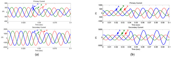
Figure 5.
External fault simulation’s primary and secondary currents: (a) the scenario of a high-voltage winding malfunction; (b) the scenario of a low-voltage winding malfunction.
5. Fault-Detection Algorithm
The differential currents are calculated from the simulated signals, and the resulting current signals are retrieved using the DWT, which is a subtraction of the primary current and the secondary current in all three phases and the zero sequence. The coefficients from each scale of DWT can be considered and used in fault detection through numerous trial-and-error processes based on the differential current of all three phases.
The DWT is applied to the 1/4 cycle of current waveforms after the fault initiation, based on a trial-and-error procedure. To decompose the high-frequency components from the current signals, the Daubechies 4 (db4) mother wavelet [54,55,56,57] is used. The coefficients of the signals obtained from the DWT are squared and studied in each scale. As shown in Figure 6, Figure 7 and Figure 8, when a fault develops, the coefficients of high-frequency components change abruptly compared to those before the fault occurs. This abrupt change is employed as a predictor of fault occurrence.
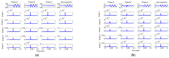
Figure 6.
In the event of an internal winding problem, DWT of differential currents from scale 1 to scale 5: (a) analysis of high-voltage winding faults; (b) analysis of low-voltage winding faults.
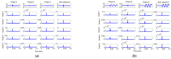
Figure 7.
In the event of an external short circuit, DWT of differential currents from scale 1 to scale 5: (a) analysis of high-voltage winding faults; (b) analysis of low-voltage winding faults.

Figure 8.
In the case of normal conditions, DWT of differential currents from scale 1 to scale 5.
Figure 6 depicts an internal fault at 20% of the winding length, while Figure 8 depicts an exterior fault at 20% of the transmission line length. The input signal is represented in Figure 6a on the top trace of the figure. As shown in Figure 6a, the input signal is a multi-signal trace from each high-pass filter that corresponds to a certain scale parameter. Figure 6 and Figure 7 indicate that the coefficients of high-frequency components change abruptly when a fault occurs compared to those before the fault occurs; yet, as shown in Figure 8, the coefficient in each scale of the DWT does not change.
The similarity between the fault signals’ waveforms from Figure 6 and Figure 7 can be seen. The result obtained from the fault-detection algorithm presumes that these signals are in their fault condition. Figure 8 shows that the coefficient at each scale of the DWT does not change. Therefore, the result obtained from the fault-detection algorithm presumes that these signals are in their normal condition. Fault detection is necessary for the decision algorithm to detect and discriminate between the power transformer’s internal and external faults. Thus, the classification of fault detection is considered. The coefficient in scale 1 from the DWT appears to be enough to indicate the fault inception, according to numerous simulations [50,51]. The coefficient in scale 1 from the DWT is utilized in many simulations [50,51] and appears to be sufficient to identify the occurrence of a fault; therefore, the coefficient in scale 1 is sufficient to train and test processes for the probabilistic neural network (PNN) without the higher-scale coefficients.
6. Decision Algorithm
The neural network toolboxes in MATLAB [60] are used to accomplish the training process. Table 2 shows how input datasets are standardized and separated into 162 sets for training and 90 sets for validation before the training process begins. The PNN’s behavior can be significantly influenced by the input pattern. As a result, the goal of this study is to use an algorithm’s input pattern to detect and distinguish between external and internal power transformer failures. The maximal coefficients of the 1/4 cycle DWT are used as training input patterns. The PNN’s output variables are labeled 1 or 2, referring to external and internal defects, respectively. The internal fault will occur if the PNN’s output value is 1. If this output value is 2, on the other hand, an external error will occur.
Table 2.
The total number of PNN datasets.
Case 1: The maximum DWT coefficients capable of detecting a fault.
A PNN structure comprises four input neurons and one output neuron, while the radial basis layer has 162 neurons (the number of neurons is always equal to the number of training sets). The input patterns for post-fault differential current waveforms are the maximum coefficients details (cD1) from DWT in the first scale at the 1/4 cycle of phase A, B, C, and zero sequence, as illustrated in Figure 9.
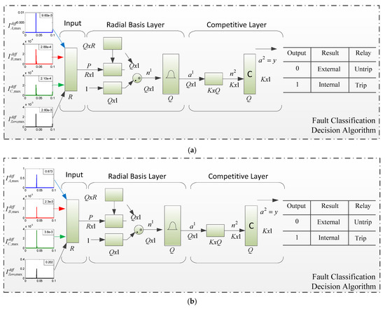
Figure 9.
PNN input pattern (maximum coefficients (cD1) in scale 1 of differential current signal): (a) case of an internal malfunction; (b) case of an external fault.
Case 2: The maximum ratio attained using the DWT division method
As illustrated in Figure 10a, the input patterns are the maximum ratio obtained from a division algorithm between the differential current coefficient from DWT and the zero sequence for post-fault differential current waveforms. In Figure 10b,c, a PNN structure consists of three neurons inputs and one neuron output, while the number of neurons in the radial basis layer is 162 (owing to the fact that the number of neurons is always equal to the number of training sets).
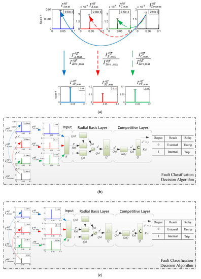
Figure 10.
PNN Input pattern of the maximum ratio in scale 1 of differential current signal: (a) the maximum ratio obtained using the division procedure provided in scale 1; (b) internal; (c) external.
During the training process [8], a normalization method uses a z-score method that has a mean of 0 and a standard deviation of 1. The z-score measures the distance of a data point from the mean in terms of the standard deviation. The standardized dataset has a mean of 0 and a standard deviation of 1, and retains the shape properties of the original dataset (same skewness and kurtosis). The z-score of a value x is . The PNN begins with the random initial weight and increasing spread in the radial basis layer, which corresponds to bias value () from 0.0001 to 0.1. The increase step of 0.0001 is used to compute the number of minimum errors. This technique is repeated until the maximum number of spreads is reached or until the number of minimal errors equals zero, at which point the training is terminated. The training procedure is depicted in Figure 11 as a flowchart, and the training outcomes are shown in Table 3.

Figure 11.
Flowchart for the training process.
Table 3.
Results of the training procedure in comparison.
Following the training procedure, the decision algorithm is used to distinguish between the different types of power transformer faults. As demonstrated in Table 4 and Table 5, case studies are modified in order to verify the decision algorithm’s capabilities. The results have two studied cases. Each studied case has 84 sets. There are 54 sets for the internal winding fault (there are 27 sets for low-voltage winding and 27 sets for high-voltage winding) and 30 sets for the external short circuit (there are 15 sets for low-voltage winding and 15 sets for high-voltage winding). The average accuracy of defect detection from the decision method suggested in this research is highly satisfactory, according to the results.
Table 4.
Percentage of internal winding fault accuracy.
Table 5.
Percentage of external winding fault accuracy.
The fault-detection methods are compared between BPNN, PNN, and RBF, the latter of which are the currently used methods of fault detection. Each method is studied in two cases in the same set. The results in Table 4 and Table 5 show the percentage of fault detection accuracy in each phase and coil distance. The average accuracies of internal winding faults in Table 4 are very close in value. Every method in every case has an accuracy of over 92.59%, most of which are up to 100%. When considering the accuracy of each method of detecting internal winding faults, it was found that PNN, BPNN, and RBF methods gave an accuracy of up to 98.15%, 98.15%, and 97.22%, respectively. The accuracy of the three methods was very similar. This supports that all three methods can be used to detect internal winding faults.
For the external winding fault detection in Table 5, the results show that the RBF method has very little accuracy compared to the other methods, with an accuracy of 21.67%. In contrast, the BPNN and PNN methods have an accuracy of 91.67% and 95%, respectively. In this study, the results of external faults showed that the PNN method gave the greatest accuracy. Therefore, it is most suitable for use in detecting external faults compared to the above methods.
Finally, when analyzing the overall test results, including internal and external faults, it was found that the PNN method provided the most accurate fault detection. As shown in Figure 12, the detection accuracy result of the PNN method is up to 193.15% from 200%, while the BPNN and RBF methods have an overall accuracy of only 189.82% and 118.89%, respectively.

Figure 12.
Comparison of the sum of detection accuracy between internal and external faults in each detection method (average of cases 1 and 2).
In a comparison of the detection methods in Figure 13, the sum of detection accuracy between internal and external faults in each detection method is compared. The results show the percentage of accuracy in detecting internal and external faults and the sum of those percentage values for each detection method. The PNN method is the most accurate in both internal and external fault detection, providing an internal fault accuracy of 98.15% and an external fault accuracy of 95%. The sum of percentage accuracy is 193.15% of 200%.
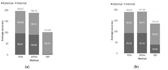
Figure 13.
Comparison of the sum of detection accuracy between internal and external faults in each case: (a) the maximum coefficients algorithm (Case 1); (b) the maximum ratio algorithm (Case 2).
Subsequently, the accuracy of the PNN method was determined in each case of the fault-detection methods consisting of the maximum coefficient algorithm (Case 1) and the maximum ratio algorithm (Case 2), as shown in Figure 13. The maximum coefficients algorithm of the PNN method provides the highest accuracy, providing an overall accuracy of 196.67% of 200%, divided into the internal fault detection accuracy within 100% and the external fault detection accuracy within 96.67%. While the maximum ratio algorithm provides an accurate analysis of the PNN and BPNN methods that are closely related, the BPNN method is slightly greater. The overall accuracy of the BPNN method is 191.49%, and the PNN method is 189.63%. The external fault detection accuracy of the PNN and BPNN methods are the same, 93.34%, while the internal fault detection accuracy of the BPNN method is 98.15%, and the PNN method is 96.30%. Therefore, from the analysis of all the test results, the PNN method is most suitable for detecting internal and external faults, and the maximum coefficient algorithm is the most effective in detecting faults.
7. Conclusions
This study investigates a new technique for detecting and distinguishing external and internal power transformer defects. This method, which uses a mix of DWT and PNN, has been presented. The DWT has been used to deconstruct high-frequency fault signal components. To compare the DWT maximum coefficient and the maximum ratio of the division algorithm, the PNN was divided into two training cases. In various circumstances, different fault kinds and locations on both the main and secondary sides of the power transformer are considered. The average accuracy of the DWT maximum coefficient cases is more than 96.67 percent, which is more satisfactory. The simulation results demonstrated that the PNN and BPNN are effectively implemented and perform fault detection with satisfactory accuracy. The PNN method’s maximum coefficients algorithm has the highest accuracy, with an internal fault detection accuracy of 100 percent and external fault detection accuracy of 96.67 percent. The maximum ratio technique gives an accurate analysis of the nearly comparable PNN and BPNN approaches; the BPNN method is significantly greater. The BPNN method has a 191.49 percent overall accuracy, while the PNN approach has a 189.63 percent overall accuracy. External fault detection accuracy is 93.34 percent for both the PNN and BPNN approaches, while internal fault detection accuracy is 98.15 percent for the BPNN method and 96.30 percent for the PNN method. However, the PNN method is most suitable for detecting internal and external faults, and the maximum coefficient algorithm is the most effective at detecting the fault. Although the suggested approach produces satisfactory results, the overall accuracy indicates that it has to be improved in order to attain higher precision. This strategy, on the other hand, will be useful in the power transformer’s differential protection scheme. The method will be improved in the future so that the transformer’s magnetizing inrush current can be determined.
Author Contributions
Conceptualization, A.N. and N.P.; methodology, N.P.; software, S.T.; validation, C.P., S.A. and M.L.; formal analysis, S.B.; investigation, V.P.; resources, P.C.; data curation, A.N.; writing—original draft preparation, S.A.; writing—review and editing, C.P. and N.P.; visualization, S.Y.; supervision, S.B.; project administration, S.Y.; funding acquisition, P.C. All authors have read and agreed to the published version of the manuscript.
Funding
This work was supported in part by the Rajamangala University of Technology Rattanakosin Research Fund.
Institutional Review Board Statement
Not applicable.
Informed Consent Statement
Not applicable.
Data Availability Statement
Data is contained within the article.
Acknowledgments
This work was supported in part by the Rajamangala University of Technology Rattanakosin Research Fund.
Conflicts of Interest
The authors declare no conflict of interest.
References
- Cano-González, R.; Bachiller-Soler, A.; Rosendo-Macías, J.A.; Álvarez-Cordero, G. Controlled switching strategies for transformer inrush current reduction: A comparative study. Electr. Power Syst. Res. 2017, 145, 12–18. [Google Scholar] [CrossRef]
- Ali, E.; Malik, O.P.; Abdelkader, S.; Helal, A.; Desouki, H. Experimental results of ratios-based transformer differential protection scheme. Int. Trans. Electr. Energy Syst. 2019, 29, e12114. [Google Scholar] [CrossRef]
- Espinoza, R.G.F.; Tavares, M.C. Faulted Phase Selection for Half-Wavelength Power Transmission Lines. IEEE Trans. Power Deliv. 2018, 33, 992–1001. [Google Scholar] [CrossRef]
- Ni, H.; Fang, S.; Lin, H. A Simplified Phase-Controlled Switching Strategy for Inrush Current Reduction. IEEE Trans. Power Deliv. 2021, 36, 215–222. [Google Scholar] [CrossRef]
- Afrasiabi, S.; Afrasiabi, M.; Parang, B.; Mohammadi, M. Designing a composite deep learning based differential protection scheme of power transformers. Appl. Soft Comput. 2020, 87, 105975. [Google Scholar] [CrossRef]
- Samet, H.; Ghanbari, T.; Ahmadi, M. An Auto-correlation Function Based Technique for Discrimination of Internal Fault and Magnetizing Inrush Current in Power Transformers. Electr. Power Compon. Syst. 2015, 43, 399–411. [Google Scholar] [CrossRef]
- Mukherjee, A.; Kundu, P.K.; Das, A. Application of Principal Component Analysis for Fault Classification in Transmission Line with Ratio-Based Method and Probabilistic Neural Network: A Comparative Analysis. J. Inst. Eng. India Ser. B 2020, 101, 321–333. [Google Scholar] [CrossRef]
- Balaga, H.; Gupta, N.; Vishwakarma, D.N. GA trained parallel hidden layered ANN based differential protection of three phase power transformer. Int. J. Electr. Power Energy Syst. 2015, 67, 286–297. [Google Scholar] [CrossRef]
- Ebadi, A.; Hosseini, S.; Abdoos, A.A. Designing of a New Transformer Ground Differential Relay Based on Probabilistic Neural Network. JEM. 2020, 9, 2–13. [Google Scholar]
- Zou, A.; Deng, R.; Mei, Q.; Zou, L. Fault diagnosis of a transformer based on polynomial neural networks. Clust. Comput. 2019, 22, 9941–9949. [Google Scholar] [CrossRef]
- Moradzadeh, A.; Pourhossein, K. Location of Disk Space Variations in Transformer Winding using Convolutional Neural Networks. In Proceedings of the 2019 54th International Universities Power Engineering Conference (UPEC), Bucharest, Romania, 3–6 September 2019; pp. 1–5. [Google Scholar]
- Fernandes, J.F.; Costa, F.B.; de Medeiros, R.P. Power transformer disturbance classification based on the wavelet transform and artificial neural networks. In Proceedings of the 2016 International Joint Conference on Neural Networks (IJCNN), Vancouver, BC, Canada, 24–29 July 2016; pp. 640–646. [Google Scholar]
- Chen, S.; Ge, H.; Li, H.; Sun, Y.; Qian, X. Hierarchical deep convolution neural networks based on transfer learning for transformer rectifier unit fault diagnosis. Measurement 2020, 167, 108257. [Google Scholar] [CrossRef]
- Afrasiabi, M.; Afrasiabi, S.; Parang, B.; Mohammadi, M. Power Transformers Internal Fault Diagnosis Based on Deep Convolutional Neural Networks. J. Intell. Fuzzy Syst. 2019, 37, 1165–1179. [Google Scholar] [CrossRef]
- Siddique, M.A.A.; Mehfuz, S. Artificial neural networks based incipient fault diagnosis for power transformers. In Proceedings of the 2015 Annual IEEE India Conference (INDICON), New Delhi, India, 17–20 December 2015; pp. 1–6. [Google Scholar]
- Nagpal, T.; Brar, Y.S. Neural network-based transformer incipient fault detection. In Proceedings of the 2014 International Conference on Advances in Electrical Engineering (ICAEE), Vellore, India, 9–11 June 2014; pp. 1–5. [Google Scholar]
- Wang, H.; Butler, K.L. Finite element analysis of internal winding faults in distribution transformers. IEEE Trans. Power Deliv. 2001, 16, 422–428. [Google Scholar] [CrossRef]
- Aker, E.; Othman, M.L.; Veerasamy, V.; Aris, I.b.; Wahab, N.I.A.; Hizam, H. Fault Detection and Classification of Shunt Compensated Transmission Line Using Discrete Wavelet Transform and Naive Bayes Classifier. Energies 2020, 13, 243. [Google Scholar] [CrossRef]
- Ehsanifar, A.; Allahbakhshi, M.; Tajdinian, M.; Dehghani, M.; Montazeri, Z.; Malik, O.; Guerrero, J.M. Transformer inter-turn winding fault detection based on no-load active power loss and reactive power. Int. J. Electr. Power Energy Syst. 2021, 130, 107034. [Google Scholar] [CrossRef]
- Hashemnia, N.; Abu-Siada, A.; Islam, S. Improved power transformer winding fault detection using FRA diagnostics – part 1: Axial displacement simulation. IEEE Trans. Dielectr. Electr. Insul. 2015, 22, 556–563. [Google Scholar] [CrossRef]
- Zhou, H.; Hong, K.; Huang, H.; Zhou, J. Transformer winding fault detection by vibration analysis methods. Appl. Acoust. 2016, 114, 136–146. [Google Scholar] [CrossRef]
- Masoum, A.S.; Hashemnia, N.; Abu-Siada, A.; Masoum, M.A.S.; Islam, S.M. Online Transformer Internal Fault Detection Based on Instantaneous Voltage and Current Measurements Considering Impact of Harmonics. IEEE Trans. Power Deliv. 2017, 32, 587–598. [Google Scholar] [CrossRef]
- Khan, S.A.; Equbal, M.D.; Islam, T. A comprehensive comparative study of DGA based transformer fault diagnosis using fuzzy logic and ANFIS models. IEEE Trans. Dielectr. Electr. Insul. 2015, 22, 590–596. [Google Scholar] [CrossRef]
- Huang, Y.; Sun, H. Dissolved gas analysis of mineral oil for power transformer fault diagnosis using fuzzy logic. IEEE Trans. Dielectr. Electr. Insul. 2013, 20, 974–981. [Google Scholar] [CrossRef]
- Abu-Siada, A.; Hmood, S. A new fuzzy logic approach to identify power transformer criticality using dissolved gas-in-oil analysis. Int. J. Electr. Power Energy Syst. 2015, 67, 401–408. [Google Scholar] [CrossRef]
- Xuewei, Z.; Hanshan, L. Research on transformer fault diagnosis method and calculation model by using fuzzy data fusion in multi-sensor detection system. Optik 2019, 176, 716–723. [Google Scholar] [CrossRef]
- Zhang, K.; Yuan, F.; Guo, J.; Wang, G. A Novel Neural Network Approach to Transformer Fault Diagnosis Based on Momentum-Embedded BP Neural Network Optimized by Genetic Algorithm and Fuzzy c-Means. Arab. J. Sci. Eng. 2016, 41, 3451–3461. [Google Scholar] [CrossRef]
- Li, E.; Wang, L.; Song, B.; Jian, S. Improved Fuzzy C-Means Clustering for Transformer Fault Diagnosis Using Dissolved Gas Analysis Data. Energies 2018, 11, 2344. [Google Scholar] [CrossRef]
- Ashrafian, A.; Rostami, M.; Gharehpetian, G.B. Hyperbolic S-transform-based method for classification of external faults, incipient faults, inrush currents and internal faults in power transformers. IET Gener. Transm. Distrib. 2012, 6, 940–950. [Google Scholar] [CrossRef]
- Yahya, Y.; Qian, A.; Yahya, A. Power Transformer Fault Diagnosis Using Fuzzy Reasoning Spiking Neural P Systems. J. Intell. Learn. Syst. Appl. 2016, 8, 77–91. [Google Scholar] [CrossRef]
- Illias, H.A.; Liang, W.Z. Identification of transformer fault based on dissolved gas analysis using hybrid support vector machine-modified evolutionary particle swarm optimisation. PLoS ONE 2018, 13, e0191366. [Google Scholar] [CrossRef]
- Zhang, W.; Yang, X.; Deng, Y.; Li, A. An Inspired Machine-Learning Algorithm with a Hybrid Whale Optimization for Power Transformer PHM. Energies 2020, 13, 3143. [Google Scholar] [CrossRef]
- Zeng, B.; Guo, J.; Zhu, W.; Xiao, Z.; Yuan, F.; Huang, S. A Transformer Fault Diagnosis Model Based on Hybrid Grey Wolf Optimizer and LS-SVM. Energies 2019, 12, 4170. [Google Scholar] [CrossRef]
- Illias, H.A.; Chai, X.R.; Bakar, A.H.A. Hybrid modified evolutionary particle swarm optimisation-time varying acceleration coefficient-artificial neural network for power transformer fault diagnosis. Measurement 2016, 90, 94–102. [Google Scholar] [CrossRef]
- Al-Janabi, S.; Rawat, S.; Patel, A.; Al-Shourbaji, I. Design and evaluation of a hybrid system for detection and prediction of faults in electrical transformers. Int. J. Electr. Power Energy Syst. 2015, 67, 324–335. [Google Scholar] [CrossRef]
- Wei, C.H.; Tang, W.H.; Wu, Q.H. A Hybrid Least-square Support Vector Machine Approach to Incipient Fault Detection for Oil-immersed Power Transformer. Electr. Power Compon. Syst. 2014, 42, 453–463. [Google Scholar] [CrossRef]
- Mejia-Barron, A.; Valtierra-Rodriguez, M.; Granados-Lieberman, D.; Olivares-Galvan, J.C.; Escarela-Perez, R. Experimental data-based transient-stationary current model for inter-turn fault diagnostics in a transformer. Electr. Power Syst. Res. 2017, 152, 306–315. [Google Scholar] [CrossRef]
- Mejia-Barron, A.; Valtierra-Rodriguez, M.; Granados-Lieberman, D.; Olivares-Galvan, J.C.; Escarela-Perez, R. The application of EMD-based methods for diagnosis of winding faults in a transformer using transient and steady state currents. Measurement 2018, 117, 371–379. [Google Scholar] [CrossRef]
- Penaloza, J.R.; Borghetti, A.; Napolitano, F.; Tossani, F.; Nucci, C. Performance analysis of a transient-based earth fault protection system for unearthed and compensated radial distribution networks. Electr. Power Syst. Res. 2021, 197, 107306. [Google Scholar] [CrossRef]
- Bera, P.K.; Isik, C.; Kumar, V. Discrimination of Internal Faults and Other Transients in an Interconnected System with Power Transformers and Phase Angle Regulators. IEEE Syst. J. 2021, 15, 3450–3461. [Google Scholar] [CrossRef]
- Zhao, X.; Yao, C.; Zhao, Z.; Abu-Siada, A. Performance evaluation of online transformer internal fault detection based on transient overvoltage signals. IEEE Trans. Dielectr. Electr. Insul. 2017, 24, 3906–3915. [Google Scholar] [CrossRef]
- Xu, J.; Gao, C.; Ding, J.; Shi, X.; Feng, M.; Zhao, C.; Ding, H. High-Speed Electromagnetic Transient (EMT) Equivalent Modelling of Power Electronic Transformers. IEEE Trans. Power Deliv. 2021, 36, 975–986. [Google Scholar] [CrossRef]
- Kariyawasam, S.; Rajapakse, A.D.; Perera, N. Investigation of Using IEC 61850-Sampled Values for Implementing a Transient-Based Protection Scheme for Series-Compensated Transmission Lines. IEEE Trans. Power Deliv. 2018, 33, 93–101. [Google Scholar] [CrossRef]
- Adly, A.R.; El-Sehiemy, R.A.; Abdelaziz, A.Y.; Kotb, S.A. An Accurate Technique for Discrimination between Transient and Permanent Faults in Transmission Networks. Electr. Power Compon. Syst. 2017, 45, 366–381. [Google Scholar] [CrossRef]
- Alexopoulos, T.; Biswal, M.; Brahma, S.M.; El Khatib, M. Detection of fault using local measurements at inverter interfaced distributed energy resources. In Proceedings of the 2017 IEEE Manchester PowerTech, Manchester, UK, 18–22 June 2017; pp. 1–6. [Google Scholar]
- Ma, J.; Wang, Z.; Yang, Q.; Liu, Y. Identifying Transformer Inrush Current Based on Normalized Grille Curve. IEEE Trans. Power Deliv. 2011, 26, 588–595. [Google Scholar] [CrossRef]
- Bagheri, S.; Moravej, Z.; Gharehpetian, G.B. Classification and Discrimination Among Winding Mechanical Defects, Internal and External Electrical Faults, and Inrush Current of Transformer. IEEE Trans. Ind. Inform. 2018, 14, 484–493. [Google Scholar] [CrossRef]
- Medeiros, R.P.; Costa, F.B. A Wavelet-Based Transformer Differential Protection with Differential Current Transformer Saturation and Cross-Country Fault Detection. IEEE Trans. Power Deliv. 2018, 33, 789–799. [Google Scholar] [CrossRef]
- Saleh, S.A.; Scaplen, B.; Rahman, M.A. A New Implementation Method of Wavelet Packet Transform Differential Protection for Power Transformers. IEEE Trans. Ind. Appl. 2011, 47, 1003–1012. [Google Scholar] [CrossRef]
- Jettanasen, C.; Ngaopitakkul, A. The spectrum comparison technique of DWT for discrimination between external fault and internal faults in Power Transformer. J. Int. Counc. Electr. Eng. 2012, 2, 302–308. [Google Scholar] [CrossRef]
- Pothisarn, C.; Jettanasen, C.; Klomjit, J.; Ngaopitakkul, A. Coefficient Comparison Technique of Discrete Wavelet Transform for Discriminating between External Short Circuit and Internal Winding Fault in Power Transformer. In Proceedings of the International MultiConference of Engineers and Computer Scientists 2012 Vol II, IMECS 2012, Hong Kong, 14–16 March 2012; pp. 1129–1134. [Google Scholar]
- Rumkidkarn, J.; Ngaopitakkul, A. Behavior analysis of winding to ground fault in transformer using high and low frequency components from discrete wavelet transform. In Proceedings of the 2017 International Conference on Applied System Innovation (ICASI), Sapporo, Japan, 13–17 May 2017; pp. 1102–1105. [Google Scholar]
- Jettanasen, C.; Pothisarn, C.; Klomjit, J.; Ngaopitakkul, A. Discriminating among inrush current, external fault and internal fault in power transformer using low frequency components comparison of DWT. In Proceedings of the 2012 15th International Conference on Electrical Machines and Systems (ICEMS), Sapporo, Japan, 21–24 October 2012; pp. 1–6. [Google Scholar]
- Apisit, C.; Ngaopitakkul, A. Identification of Fault Types for Underground Cable using Discrete Wavelet Transform. In Proceedings of the International MultiConference of Engineers and Computer Scientists 2010 Vol II, IMECS 2010, Hong Kong, 17–19 March 2010. [Google Scholar]
- Klomjit, J.; Ngaopitakkul, A.; Sreewirote, B. Comparison of mother wavelet for classification fault on hybrid transmission line systems. In Proceedings of the 2017 IEEE 8th International Conference on Awareness Science and Technology (iCAST), Taichung, Taiwan, 8–10 November 2017; pp. 527–532. [Google Scholar]
- Pothisarn, C.; Klomjit, J.; Ngaopitakkul, A.; Jettanasen, C.; Asfani, D.A.; Negara, I.M.Y. Comparison of Various Mother Wavelets for Fault Classification in Electrical Systems. Appl. Sci. 2020, 10, 1203. [Google Scholar] [CrossRef]
- Ngaopitakkul, A.; Kunakorn, A. Internal Fault Classification in Transformer Windings using Combination of Discrete Wavelet Transforms and Back-Propagation Neural Networks. Int. J. Control. Autom. Syst. 2006, 4, 365–371. [Google Scholar]
- Kanirajan, P.; Kumar, V.S. Power quality disturbance detection and classification using wavelet and RBFNN. Appl. Soft Comput. 2015, 35, 470–481. [Google Scholar] [CrossRef]
- Patcharoen, T.; Ngaopitakkul, A. Transient Inrush Current Detection and Classification in 230 kV Shunt Capacitor Bank Switching Under Various Transient Mitigation Methods Based on Discrete Wavelet Transform. IET Gener. Transm. Distrib. 2018, 12, 3718–3725. [Google Scholar] [CrossRef]
- Demuth, H.; Beale, M. Neural Network Toolbox User’s Guide; The Math Work, Inc.: Natick, MA, USA, 2001. [Google Scholar]
- Bastard, P.; Bertrand, P.; Meunier, M. A transformer model for winding fault studies. IEEE Trans. Power Deliv. 1994, 9, 690–699. [Google Scholar] [CrossRef]
- IEEE Working Group 15.08.09. Modeling and Analysis of System Transients Using Digital Programs; IEEE PES Spec. Publ.: Piscataway, NJ, USA, 1998. [Google Scholar]


Publisher’s Note: MDPI stays neutral with regard to jurisdictional claims in published maps and institutional affiliations. |
© 2021 by the authors. Licensee MDPI, Basel, Switzerland. This article is an open access article distributed under the terms and conditions of the Creative Commons Attribution (CC BY) license (https://creativecommons.org/licenses/by/4.0/).