A Convenient Way to Determine the Optimum Angle of Incidence of Fizeau Interferometer

Abstract

In a Fizeau interferometer, off-axis illumination will lead to fringe optimization. Primarily due to the unique structure of our interferometer, we first analyze the influence of the optical properties of the parallel plate as a part of the interferometer on the optimal incident angle. Generally, the incident angle determination is mainly based on the graphing method proposed by Langenbeck and the estimation formula proposed by Kajava. However, Langenbeck’s method is cumbersome, and the error of Kajava’s estimation formula is large. Based on the predecessors, this paper proposes a modified method of determining the optimal angle of incidence and further derives more accurate optimal angle expressions than Kajava’s. By simply substituting the wedge angle of the wedge cavity and the reflectivity of the cavity, the optimum incidence angle can be obtained immediately. Thus, it eliminates the tedious and complex process of finding the optimum incident angle by graphing method and makes the formula method the simplest method to find the optimum incident angle. Finally, the comparison of the interference intensity at the optimum incidence angle calculated by the improved method and normal incidence is given. It is found that the beam has a good suppression effect on the sub-peak when it is incident at the optimum incident angle calculated by the method in this paper.

1. Introduction

Fizeau interferometer has the characteristics of high resolution and high light gathering ability, so spectroscopy workers have always valued it. In 2011, Frédéric Gillard and Sidonie Lefebvre proposed a static Fourier transform spectrometer using an optical wedge to generate optical path difference [1,2,3,4,5,6,7]. The structure integrates an infrared area array detector with a wedge prism and uses the principle of optical path difference generated by optical wedge for infrared spectrum detection. However, this structure still needs chemical etching after coating, and it requires high precision of the working surface. In order to realize the marketization and popularization of the spectrometer, based on the wedge structure, this paper proposes an improved Fizeau spectrometer structure with simple manufacture and lower cost. As shown in Figure 1, a parallel plate coated with high reflection film is pasted on the focal plane array. There is a wedge-shaped air chamber with angle α composed by this parallel plate and another parallel plate also plated with high reflection film. Due to the sudden refractive index change at the air/plate interface, the light is reflected inside the wedge, and the multi-beams transmitted and reflected in the wedge will interfere. The focal plane array records the interference fringes, and then the incident spectrum is solved by corresponding algorithms.

However, if the collimated light is directly incident on the Fizeau interference system, there is a sub-peak in the interference fringe received by the detector [8,9,10,11,12]. During spectral inversion, the intensity of the sub-peak will be superimposed on the intensity of the prominent peak of other wavelengths to reduce the accuracy of spectral inversion. Predecessors have done much research on eliminating the sub-peak. The general idea is to find an optimum incidence angle. When the collimated light is incident at this angle, the influence of the sub-peak will be reduced or even eliminated. In terms of determining the optimum incident angle, the graphing method of the sum of the amplitude vector proposed by Langenbeck and the estimation formula proposed by Kajava is mainly used to select the optimum incident angle [13,14]. Langenbeck uses the relationship between the phase and the sum of the amplitude vector to make a plot. Then find the value of the incident angle when the sum of amplitude vector is the largest as the optimum incident angle. Kajava proposed a formula for the optimum incident angle in 1993 based on understanding the multi-beam intensity distribution involved in the interference in the Fizeau interferometer. The two methods have their own advantages and disadvantages. Firstly, the sum of amplitude vector graphing method has high accuracy in determining the optimum incidence angle, which is the most commonly used method to determine the optimum incidence angle at present. However, the process is cumbersome and complicated. The formula mentioned by Kajava can immediately obtain the value of the optimum incident angle by simply substituting the structural parameters. Nevertheless, the error of the optimum incident angle obtained by this formula is significant. Moreover, due to the special structure of the spectrometer mentioned in this paper, the incident beam is reflected many times in the wedge cavity and emitted through the parallel plate. The phase of each outgoing beam will be modulated by the thickness and refractive index of the parallel plate, resulting in the change of spatial interference intensity, which may lead to the deviation of the optimum incident angle. Furthermore, the theory of finding the optimum incident angle by predecessors such as Langenbeck and Kajava did not consider the influence of parallel plates. Generally, the models that can be used to describe the spatial distribution of light include the brightness model of random field and the model of plane wave superposition and interaction in space [15]. In this paper, using the second model, firstly, the influence of parallel plate on spatial interference intensity modulation when parallel beam is incident on Fizeau interferometer system is studied theoretically. It is proposed that if the thickness of the parallel plate behind the wedge cavity cannot be ignored, the spatial interference intensity distribution will have an intensity reproduction along the longitudinal direction from the rear surface of the parallel plate.

In particular, based on predecessors, an improved method was proposed for finding the optimum incident angle by finding the extreme point of the relationship between the sum of amplitude vector of the point and the incident angle. On this basis, a more exact expression formula of the optimum incidence angle is also derived. By simply substituting the value of the wedge angle and the reflectivity of the wedge cavity, the accurate value of the optimum incidence angle can be obtained immediately. Thus, it eliminates the tedious and complex process of finding the optimum incident angle by graphing method and makes the formula method the most straightforward choice for finding the optimum incident angle. This method of determining the optimal incident angle is expected to be used to evaluate the optimal laser exposure angle position [16,17]. The structure of this paper is as follows: In the second section, we analyze the modulation effect of the thickness of the parallel plate behind the wedge cavity on the spatial light intensity distribution and theoretically analyze the influence of the parallel plate on the value of the optimum incident angle. In the third section, we introduce the influence of various factors on the interference intensity and the reasons for the appearance of interference intensity sidelobes. An improved graphing method is proposed to correct the distortion interference intensity by calculating the pole of the relationship between the sum of vector amplitude and incident angle. Based on this method, a more accurate estimation expression of the optimum incident angle is obtained. In Section 4, the optimum incidence angle obtained by the formula is compared with that obtained by the graphing method and Kajava’s formula. It is found that the results obtained by the formula method are in good agreement with those obtained by the graphing method.

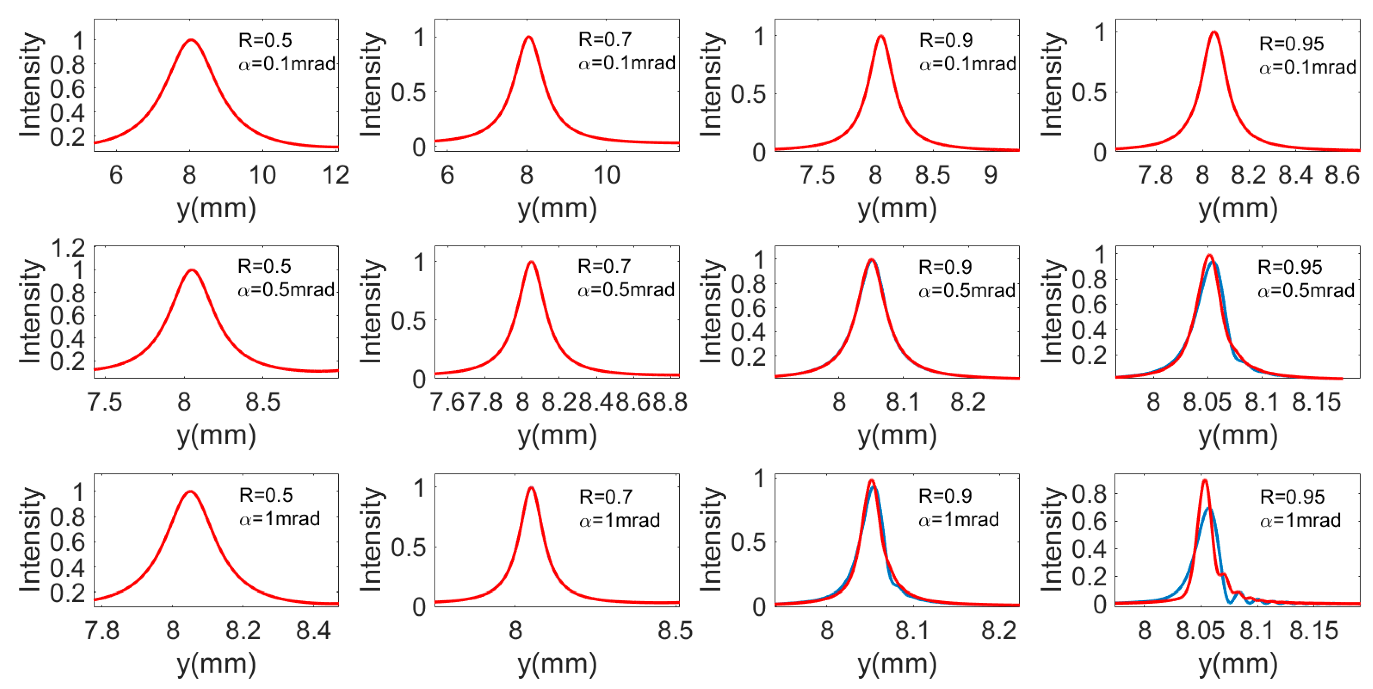
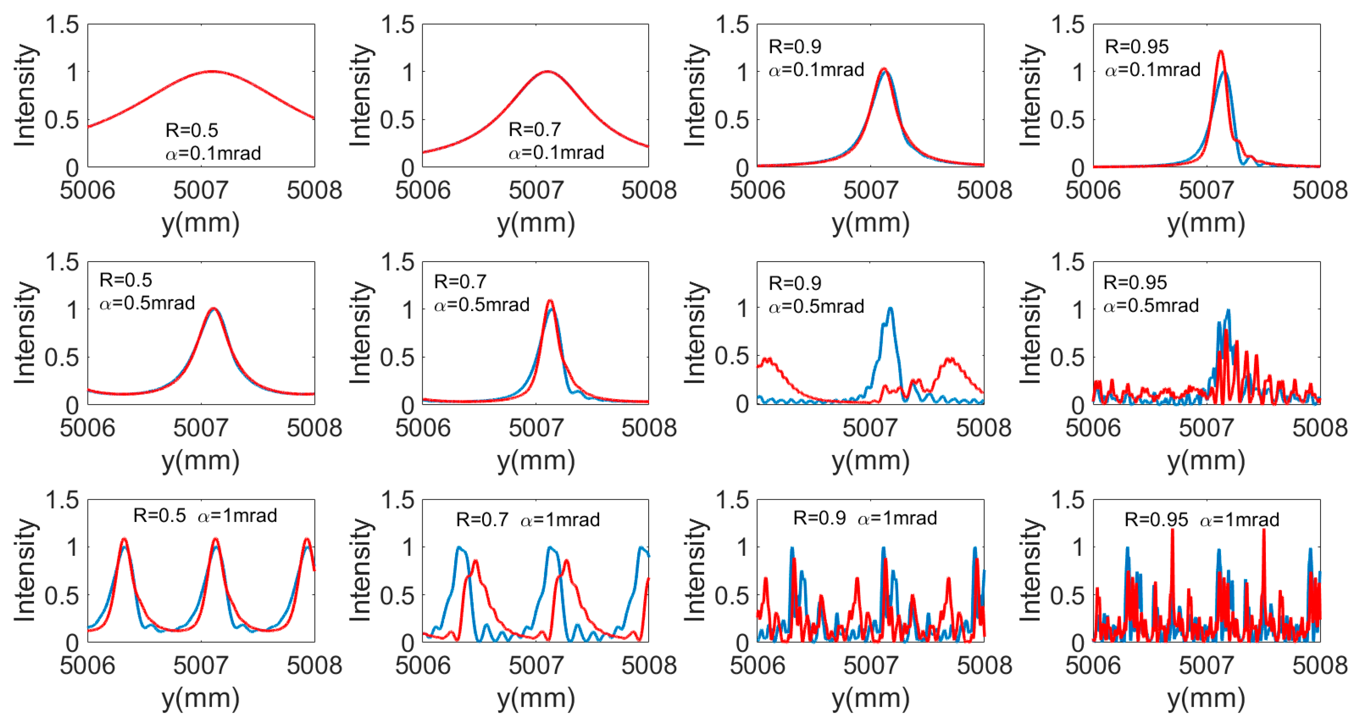
2. Analysis of Spatial Light Intensity Distribution

The interference intensity distribution made by predecessors is based on the simple wedge structure, and the influence of the specific composition structure of the wedge cavity on the spatial interference intensity is not considered [18,19]. Based on the specific design structure of our spectrometer, since the parallel plate close to the telescope system is a non-focal system and does not participate in the interference optical path, this paper does not analyze the contribution of this parallel plate to the optical path. The parallel plate near the focal plane array is directly involved in the interference light path, which leads us to analyze the influence of the parallel plate on the interference light intensity distribution. As shown in Figure 2, an ideal collimated beam enters the interferometer, and the angle between the incident beam and the normal on the back of the wedge cavity is the incident angle θ. Here, it is specified that the angle of clockwise rotation of the optical axis to the incident direction is negative; conversely, θ is positive. The incident plane wave is repeatedly reflected into a series of beams in the wedge cavity. These plane waves are in phase with the beams mentioned above, but their propagation directions are twice α different from each other, and the strength decreases exponentially. However, due to the influence of the parallel plate on the optical path, the light is refracted at the interface between the parallel plate and the air, and the angle between the incident light and the mth outgoing light is no longer a simple 2mα. When the beam exits from the parallel plate, due to the non-focus of the parallel plate, the direction of the outgoing beam is consistent with the direction of the beam incident on the parallel plate. However, since the beam passes through the parallel plate, the spatial interference intensity distribution of a point in space is related to the thickness and refractive index of the parallel plate. Here, we assume that a point in space is $P\left(z_0,y_0\right)$. The amplitude distribution of point P is only related to the relative phase difference between the reflected wavefront. It is assumed that the optical path from the incident wavefront and the optical path from the mth outgoing wavefront to P is $L_0$ and $L_m$, respectively. Both reflectivities in the wedge cavity are R, and the thickness of the parallel plate is d. When P is inside the wedge cavity $\left(0\le z_0\le d\right)$, the optical path expression from the incoming wavefront and the mth outgoing wavefront to point P can be calculated, respectively.

$$L_0=z_0{\left(n^2-si{n}^2\theta \right)}^{\frac{1}{2}}+y_{0}sin\theta$$

(1)

$$L_m=z_0{\left(n^2-si{n}^2\left(\theta +2m\alpha \right)\right)}^{\frac{1}{2}}+y_{0}sin\left(\theta +2m\alpha \right)$$

(2)

where n is the refractive index of the parallel plate, and α is the apex angle of the wedge cavity. The optical path difference between the incident wavefront and the mth outgoing wavefront to point P is

$$\begin{gathered} \Delta L=L_m-L_0 \\ =y_0\left(sin\left(\theta +2m\alpha \right)-sin\theta \right)+z_0\left({\left(n^2-si{n}^2\left(\theta +2m\alpha \right)\right)}^{\frac{1}{2}}-{\left(n^2-si{n}^2\theta \right)}^{\frac{1}{2}}\right) \end{gathered}$$

(3)

when the beam exits from a parallel plate $\left(z_0\ge d\right)$, the optical path from the incident wavefront and the mth exit wavefront to point P satisfies

$$L_0=\left(z_0-d\right)·cos\theta +y_0·sin\theta +d·\sqrt{n^2-si{n}^2\theta }$$

(4)

$$\begin{gathered} L_m=\left(z_0-d\right)·cos\left(\theta +2m\alpha \right)+y_0·sin\left(\theta +2m\alpha \right)+d \\ ·\sqrt{n^2-si{n}^2\left(\theta +2m\alpha \right)} \end{gathered}$$

(5)

At this time, the optical path difference between the incident wavefront and the mth outgoing wavefront to point P is

$$\begin{array}{cc}\hfill \Delta L=L_m-L_0=& \left(z_0-d\right)·\left(cos\left(\theta +2m\alpha \right)-cos\theta \right)+y_0\hfill \\ & ·\left(sin\left(\theta +2m\alpha \right)-sin\theta \right)+d\hfill \\ & ·\left(\sqrt{n^2-si{n}^2\left(\theta +2m\alpha \right)}-\sqrt{n^2-si{n}^2\theta }\right)\hfill \end{array}$$

(6)

when mα approaching zero, Equation (6) can be expressed in a simplified form by use of the Taylor-series expansion

$$sin\left(2m\alpha \right)=2m\alpha -\frac{{\left(2m\alpha \right)}^3}{6}+o{\left(2m\alpha \right)}^5$$

(7)

$$cos\left(2m\alpha \right)=1-\frac{{\left(2m\alpha \right)}^2}{2}+\frac{{\left(2m\alpha \right)}^4}{24}+o{\left(2m\alpha \right)}^6$$

(8)

In the approximation we collect all the term in Equations (7) and (8) up to the second power of $m\alpha$. The optical path difference between the incident wavefront and the mth outgoing wavefront to point P becomes

$$\Delta L=\{\begin{array}{c}2m\alpha ·y_0-\left(\frac{2m\theta \alpha }{n}+\frac{2m^2{\alpha }^2}{n} \right)·z_0 \hspace{1em}\hspace{1em}\hspace{1em}\hspace{1em}\hspace{1em}{z}_0\in \left[0,d\right]\\ 2m\alpha ·y_0-\left(2m\alpha \theta +2m^2{\alpha }^2 \right)·\left(z_0+\left(\frac{1}{n}-1\right)·d\right)z_0\in \left(d,\infty \right)\end{array}$$

(9)

If the amplitude transmission coefficient of the parallel plate surface close to the focal plane array is t, the amplitude spatial distribution is

$$\begin{gathered} E\left(y_0,z_0\right)= \\ \{\begin{array}{c}{E}_0{\displaystyle {\displaystyle \sum }_{m=0}^M}{R}^{m}exp\left\{ik\left[2m\alpha ·y_0-\left(\frac{2m\theta \alpha }{n}+\frac{2m^2{\alpha }^2}{n} \right)·z_0\right]\right\} z_0\in \left[0,d\right]\\ E_0{\displaystyle {\displaystyle \sum }_{m=0}^M}t{R}^{m}exp\left\{ik\left[2m\alpha ·y_0-\left(2m\alpha \theta +2m^2{\alpha }^2 \right)·\left(z_0+{\epsilon }_z·d\right)\right]\right\} z_0\in \left(d,\infty \right)\end{array} \end{gathered}$$

(10)

Among ${\epsilon }_z=\frac{1}{n}-1$. Under the paraxial condition, the spatial distribution of amplitude is

$$E\left(y_0,z_0\right)=\{\begin{array}{c}{E}_0{\displaystyle {\displaystyle \sum }_{m=0}^M}{R}^{m}exp\left\{ik\left[2m\alpha ·y_0-\frac{2m^2{\alpha }^2}{n}·z_0\right]\right\} z_0\in \left[0,d\right]\\ E_0{\displaystyle {\displaystyle \sum }_{m=0}^M}t{R}^{m}exp\left\{ik\left[2m\alpha ·y_0-2m^2{\alpha }^2·\left(z_0+{\epsilon }_z·d\right)\right]\right\} z_0\in \left(d,\infty \right)\end{array}$$

(11)

According to the characteristic that the amplitude weight decreases in geometric series, we can select a certain number of effective beams according to the estimation error. When the strength error is $\left|\frac{err\left(I\right)}{I}\right|\le \epsilon$, the number of effective beams is [18]

$$M=lo{g}_R\left(\frac{\epsilon \left(1-\mathrm{R}\right)}{2\left(1+\mathrm{R}\right)}\right)$$

(12)

It can be seen from Equation (11) that in any medium, the lattice period along the transverse direction is not affected by the refractive index n of the medium. However, along the longitudinal direction, the lattice period is related to the material’s refractive index, as shown in Figure 3. In fact, in this case, the distribution position of spatial interference intensity in the longitudinal direction has an n-fold relationship with the coordinates of the corresponding position in the air. Suppose there is a focal plane array in a parallel plate, the relationship between the value of the optimum incidence angle ${\theta }_{Opt\_P}$ and the optimum incidence angle ${\theta }_{Opt\_A}$ when the parallel plate does not exist is satisfied:

$${\theta }_{Opt\_P}=n{\theta }_{Opt\_A}$$

(13)

when the plane waves of all levels exit from the parallel plate and form the interference intensity in space, the intensity distribution compared with the absence of parallel plate phase modulation shifts. Overall, the strength distribution shifts to the right along the longitudinal direction by a distance of ${\epsilon }_z·d$, and this distance is marked with a red dotted line in Figure 4. The period of spatial coherence distribution is not affected by the parallel plate, so the optimum incidence angle ${\theta }_{Opt\_P}$ is the same as the optimum incidence angle ${\theta }_{Opt\_A}$ when the parallel plate does not exist, that is

$${\theta }_{Opt\_P}={\theta }_{Opt\_A}$$

(14)

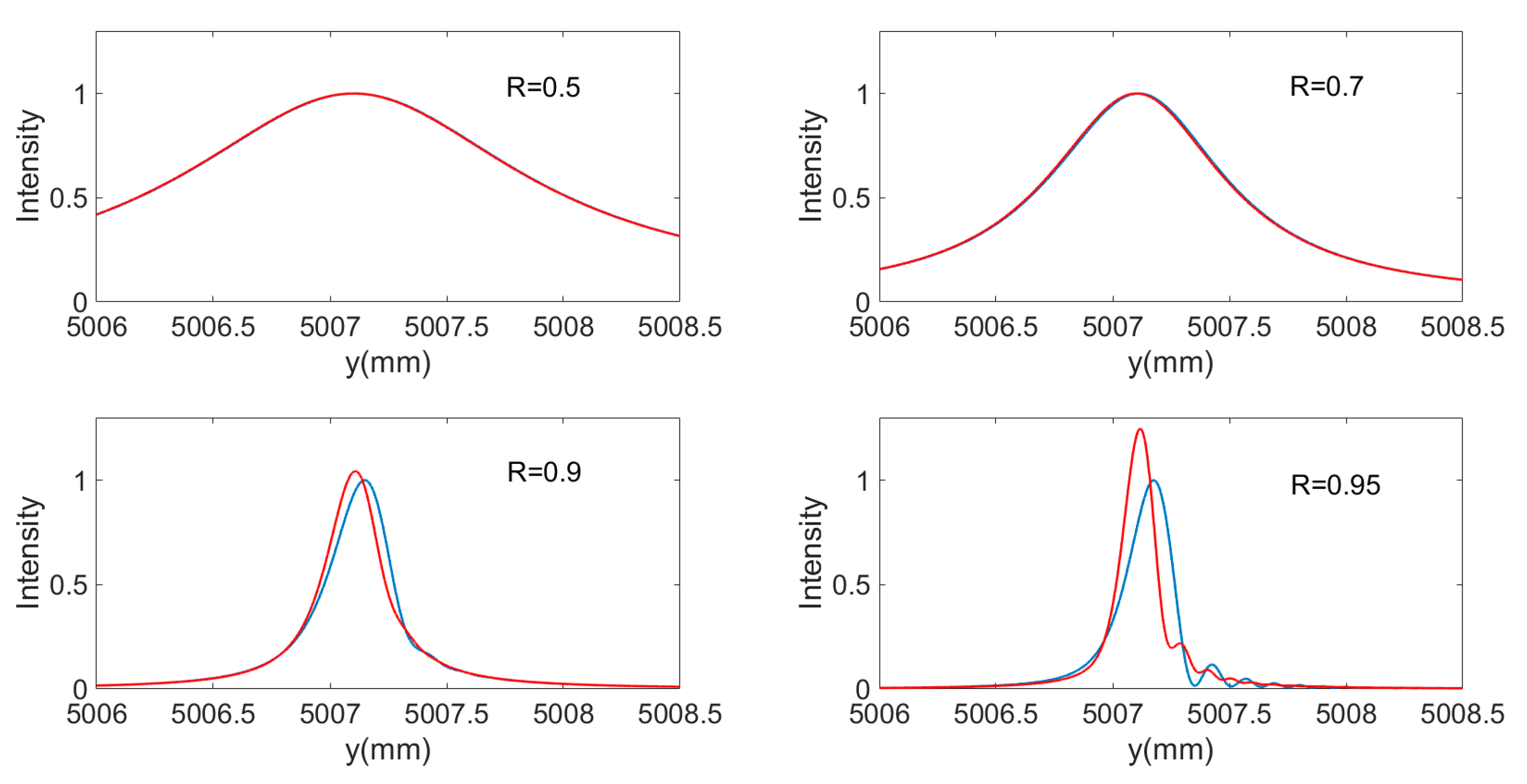
3. Determination of the Optimum Incident Angle

Based on the influence of the thickness of parallel plates on the spatial interference intensity distribution analyzed in Section 2, it is found that there is an expression of a coordinate transformation based on the point of rotation θ in the formula. In this case, the optimal incident angle when the beam passes through the parallel plate and interferes behind the parallel plate is equal to the optimal incident angle when the parallel plate does not exist. Unlike the symmetrical structure of a single fringe of the Fabry Perot interferometer, the Fizeau interferometer’s fringe has an asymmetric shape and substructure. The reason for fringe distortion is that the structure is unstable, making the interference beam move in the direction of increasing plate spacing so that the beam gradually dephases [20]. When α is unchanged, with the increase of y, the sub-peak will gradually appear on one side of the main peak. During spectral inversion, the intensity of the side lobe will be superimposed on the intensity of the main peak of other wavelength interferograms, resulting in inversion distortion and reducing the accuracy of spectral measurement. This situation should be avoided in the field of spectral measurement. Observing the phase distribution formula, when the wedge air layer rotates around the wedge apex o, the fringe pattern remains unchanged, which is still formed by the interference between the same wavefront. Different portions of the interference light intensity are introduced into the focal plane by the change in the incident angle θ. Thus we need to find an incident angle ${\theta }_{Opt}$, so that the focal plane is just coincident with the localized plane. Under the inclined illumination, the lattice period is not affected because it is only determined by the wedge α. In this paper, based on the research theory of LangenBeck, a more accurate method of determining the optimum entry angle is proposed. Since the natural period of the lattice point in the y-direction is λ/2α, we select the peak value closest to the wedge apex in the y-direction as the reference strength. While θ is changing, the intensity at different positions of the peak can always be introduced into the focal plane. When the intensity is maximum, the θ is the optimum incident angle we are looking for. The specific approach is taking the straight line on the rear surface of the wedge-shaped cavity, which is also perpendicular to the ridge of the wedge-shaped cavity as the reference direction. A position with a phase difference of $\pi /\alpha$ from the ridge of the wedge cavity is found in this direction. The sum of the amplitude vector here is used as the reference value. The amplitude derivative here must satisfy

$$\begin{array}{cc}\hfill \frac{dE}{d\theta }={\displaystyle {\displaystyle \sum }_{m=0}^M}{R}^{m}sin& \left[\frac{\pi }{\alpha }\left(sin\left({\theta }_{Opt}+2m\alpha \right)-sin{\theta }_{Opt}\right)\right]\hfill \\ & ·\left[\left(cos\left({\theta }_{Opt}+2m\alpha \right)-cos{\theta }_{Opt}\right)\right]=0\hfill \end{array}$$

(15)

Due to the complexity of the Equation (13), the solution of the equation can be determined by the intersection of the function plot on the left side of the equation and the horizontal axis. Compared with Langenbeck’s method of indirectly determining the optimum incidence angle by graphing the relationship between amplitude vector and phase, the improved method proposed here can find the solution of the equation by determining the intersection point, which can more intuitively and accurately determine the optimum incidence angle. Figure 5 shows the optimum incident angle obtained by plotting when the reflectivity is 0.5, 0.7, and 0.9 under different wedge angles. The red dot marked in Figure 5 is the optimum incident angle obtained by plotting when the reflectivity is 0.5, 0.7, and 0.9 under different wedge angles.

When determining the optimum incident angle, whether different graphing methods are accurate or not, the process is cumbersome. Kajava et al. tried to obtain the optimum incidence angle directly by formula method and gave an estimation formula of the optimum incidence angle.

$${\theta }_{Opt}=\frac{{{\displaystyle \sum }}_{m=0}^{\infty }\left(2m\alpha \right)R^m}{{{\displaystyle \sum }}_{m=0}^{\infty }{R}^m}\approx \frac{2\alpha R}{1-R}$$

(16)

However, since the estimation formula derived by Kajava is quite different from the value of the optimum incidence angle obtained by the graphing method, the latter method to determine the optimum incidence angle is still the mainstream method at present. In order to solve the problem of insufficient accuracy of the formula method, the left side of the equation is expanded into a fourth-order term by using Taylor expansion, which can obtain a more accurate formula ${\theta }_{Opt}$ estimator.

$${\theta }_{Opt}=\frac{\alpha {{\displaystyle \sum }}_{m=0}^{\infty }{m}^4{R}^m}{{{\displaystyle \sum }}_{m=0}^{\infty }{m}^3{R}^m}$$

(17)

Formally, the estimation formula derived in this paper is consistent with that derived by Kajava et al. In essence, both formulas estimate the average direction of the intensity of the interference wavefront. By expanding

$${\left(R^{m+4}\right)}^{\left(4\right)}=\frac{\left(m+4\right)!}{m!}{R}^m$$

(18)

$${\left(R^{m+3}\right)}^{\left(3\right)}=\frac{\left(m+3\right)!}{m!}{R}^m$$

(19)

$${\left(R^{m+2}\right)}^{\left(2\right)}=\frac{\left(m+2\right)!}{m!}{R}^m$$

(20)

$${\left(R^{m+1}\right)}^{\prime }=\left(m+1\right)R^m$$

(21)

and iterating into Equation (15), an expression after summation can be obtained

$${\theta }_{Opt}=\frac{-\alpha \left(R^3+11R^2+11R+1\right)}{\left(R^3+3R^2-3R-1\right)}$$

(22)

When θ changes, the intensities of the main peak and the sub-peak appearing in the focal plane also change. Nevertheless, regardless of the value of the incident angle, the total energy of the light on the focal plane array is constant. In other words, the lower energy of the main peak is due to the leakage of energy into the sub-peak, increasing the intensity of the sub-peak. Conversely, if the intensity of the main peak is on the increase, the power of the sub-peak will decrease. Figure 6 shows the trend of the intensity of the main peak with the incident angle θ. It can be found that when θ is equal to ${\theta }_{Opt}$, the sum of the amplitude vector of the main peak will be maximized, and the influence of the sub-peak will be minimized at this time. This plot verifies the correctness of the optimum incident angle obtained by our formula method.

As shown in Figure 7, it is the curve of the optimum incident angle obtained by Langenbeck’s graphing method, Kajava formula method, and the formula method in this paper under different wedge angles and different reflectivity. It should be noted here that due to the different number of beams involved in an interference, the average direction of intensity obtained must not be consistent. Considering this factor, the number of effective beams in the three methods is unified as M = 100 in the figure. Through comparison, it is found that under different conditions, the optimum incidence angle obtained by Langenbeck’s method is in good agreement with the optimum incidence angle determined by the formula method proposed in this paper. At the same time, there is a large gap between the value obtained by Kajava’s formula and the optimum incidence angle obtained by Langenbeck’s method.

4. Intensity Optimization

According to expression $\frac{dE}{d\theta }$, when the value of reflectivity or wedge angle is relatively low, the variation trend of the sum of the amplitude vector is insensitive to the change of $\theta$ near the optimum incidence angle. Only when R is relatively large (e.g., R is greater than 0.9) or wedge angle is relatively large (e.g., α is greater than 0.5 mrad), the difference of the sum of amplitude vector between oblique incidence and normal incidence can be clearly seen. In order to verify the effectiveness of the formula proposed in this paper, Figure 8 is the comparison diagram of the interference intensity before and after correction when the focal plane array is at z = 0 and the focal plane array is within 10 mm from the wedge apex. Compared with the direct normal incidence of the beam into the wedge cavity, the intensity of the sub-peak is significantly reduced, and the intensity of the main peak is improved when the beam is incident at the optimum incidence angle.

However, when the selected position of y is relatively large, only under the condition of a slight wedge angle or low value of reflectivity, the beam incident at the optimum incident angle will have a good correction effect on the interference intensity. Like in the case of α = 0.1 mrad, a better correction can be obtained at the peak of y = 5007 mm. However, in the case of high reflectivity (such as R = 0.9 or R = 0.95), when α > 0.5 mrad, the interference intensity has not been well corrected. Especially when the reflectivity is greater than 0.9, and the wedge angle is greater than 0.5 mrad, the interference intensity has lost the characteristics of the periodic distribution. These features can be easily seen in Figure 9. The reason for the fringe distortion is that the structural instability makes the interference beam move in the direction of increasing the plate spacing so that the beam gradually dephases. This dephasing is mainly related to two parameters. High reflectivity and large wedge angle will aggravate the dephasing of interference intensity in the y-direction. This dephasing phenomenon is caused by the structure of the Fizeau interferometer itself and can’t be corrected by changing the incident angle of the beam.

At present, the design angle of the wedge-shaped cavity is 0.1 mrad, and the thickness of the parallel plate constituting the wedge-shaped cavity is 10 mm, so it is necessary to analyze the fringe correction effect under the specific structure. Here we simulate the comparison of light intensity before and after correction when the thickness of the parallel plate is d = 10 mm, as shown in Figure 10. It is found that when the reflectivity is 0.5, 0.7, 0.9, and 0.95, respectively, the optimum incidence angle obtained by the formula still has a good correction effect on the intensity distribution.

5. Conclusions

In this paper, the modulation effect of the parallel plate on spatial interference intensity distribution in the Fizeau interferometer system is analyzed theoretically. It is found that if the focal plane array is behind the parallel plate, the optimum incidence angle is the same as that when the parallel plate does not exist. Moreover, based on previous studies, this paper proposes an improved calculation method of the optimal incidence angle and obtains a more accurate estimation formula of the optimal incidence angle. Therefore, we no longer need to use the cumbersome graphing method to determine the optimum incidence angle, which makes it fast and straightforward to decide on the optimum incidence angle.

References

1. Gillard, F.; Ferrec, Y.; Guérineau, N.; Rommeluère, S.; Taboury, J.; Chavel, P. Angular acceptance analysis of an infrared focal plane array with a built-in stationary Fourier transform spectrometer. JOSA A 2012, 29, 936–944. [Google Scholar] [CrossRef] [PubMed] [Green Version]
2. Guerineau, N.; Rommeluere, S.; Deschamps, J.; De Borniol, E.; Million, A.; Chamonal, J.P.; Destefanis, G. Infrared focal plane array with a built-in stationary fourier-transform spectrometer: First experimental results. In Proceedings of the Fourier Transform Spectroscopy, Alexandria, VA, USA, 31 January–3 February 2005. [Google Scholar]
3. Guerineau, N.; Suffis, S.; Cymbalista, P.; Primot, J. Conception of a stationary Fourier transform infrared spectroradiometer for field measurements of radiance and emissivity. In Proceedings of the Optical Design and Engineering, St. Etienne, France, 18 February 2004; Volume 5249, pp. 441–448. [Google Scholar]
4. Gillard, F.; Rommeluère, S.; de la Barrière, F.; Druart, G.; Guérineau, N.; Ferrec, Y.; Lefebvre, S.; Fendler, M.; Taboury, J. Towards a handheld cryogenic FTIR spectrometer. In Proceedings of the Fourier Transform Spectroscopy, Toronto, ON, Canada, 10–14 July 2011. [Google Scholar]
5. Ferrec, Y.; Rommeluère, S.; Lefebvre, S.; Benoît, C.; Gillard, F.; Guérineau, N. Infrared focal plane array with a built-in stationary Fourier-transform spectrometer (MICROSPOC): Physical limitations and numerical solutions. In Proceedings of the Fourier Transform Spectroscopy, Toronto, ON, Canada, 10–14 July 2011. [Google Scholar]
6. Ferrec, Y.; de la Barrière, F.; le Coarer, E.; Diard, T.; Guérineau, N.; Martin, G.; Rommeluère, S.; Schmitt, B.; Thomas, F. Current status and perspectives for Microspoc, the miniature Fourier transform spectrometer. In Proceedings of the Fourier Transform Spectroscopy, Lake Arrowhead, CA, USA, 1–4 March 2015. [Google Scholar]
7. Rommeluère, S.; Haïdar, R.; Guérineau, N.; Deschamps, J.; De Borniol, E.; Million, A.; Chamonal, J.P.; Destefanis, G. Single-scan extraction of two-dimensional parameters of infrared focal plane arrays utilizing a Fourier-transform spectrometer. Appl. Opt. 2007, 46, 1379–1384. [Google Scholar] [CrossRef] [PubMed]
8. Novák, O.; Falconer, I.S.; Sanginés, R.; Lattemann, M.; Tarrant, R.N.; McKenzie, D.R.; Bilek, M.M.M. Fizeau interferometer system for fast high-resolution studies of spectral line shapes. Rev. Sci. Instrum. 2011, 82, 023105. [Google Scholar] [CrossRef] [PubMed]
9. Bae, W.; Kim, Y. Phase extraction formula for glass thickness measurement using Fizeau interferometer. J. Mech. Sci. Technol. 2021, 35, 1623–1632. [Google Scholar] [CrossRef]
10. Kim, Y.; Hibino, K.; Sugita, N.; Mitsuishi, M. Error-compensating phase-shifting algorithm for surface shape measurement of transparent plate using wavelength-tuning Fizeau interferometer. Opt. Lasers Eng. 2016, 86, 309–316. [Google Scholar] [CrossRef]
11. Emadi, A.; Wu, H.; de Graaf, G.; Wolffenbuttel, R. Design and implementation of a sub-nm resolution microspectrometer based on a Linear-Variable Optical Filter. Opt. Express 2012, 20, 489–507. [Google Scholar] [CrossRef] [PubMed] [Green Version]
12. DeCorby, R.G.; Ponnampalam, N.; Epp, E.; Allen, T.; McMullin, J.N. Chip-scale spectrometry based on tapered hollow Bragg waveguides. Opt. Express 2009, 17, 16632–16645. [Google Scholar] [CrossRef] [PubMed]
13. Langenbeck, P. Fizeau interferometer–fringe sharpening. Appl. Opt. 1970, 9, 2053–2058. [Google Scholar] [CrossRef] [PubMed]
14. Kajava, T.T.; Lauranto, H.M.; Friberg, A.T. Interference pattern of the Fizeau interferometer. JOSA A 1994, 11, 2045–2054. [Google Scholar] [CrossRef]
15. Vasil’ev, K.K.; Dement’ev, V.E.; Andriyanov, N.A. Doubly stochastic models of images. Pattern Recognit. Image Anal. 2015, 25, 105–110. [Google Scholar] [CrossRef]
16. Shirokanev, A.S.; Kibitkina, A.S.; Ilyasova NY, E.; Degtyaryov, A.A. Methods of mathematical modeling of fundus laser exposure for therapeutic effect evaluation. Comput. Opt. 2020, 44, 809–820. [Google Scholar] [CrossRef]
17. Shirokanev, A.S.; Andriyanov, N.A.; Ilyasova, N.Y. Development of vector algorithm using CUDA technology for three-dimensional retinal laser coagulation process modeling. Comput. Opt. 2021, 45, 427–437. [Google Scholar] [CrossRef]
18. Brossel, J. Multiple-beam localized fringes: Part I.-Intensity distribution and localization. Proc. Phys. Soc. 1947, 59, 224. [Google Scholar] [CrossRef]
19. Brossel, J. Multiple-beam localized fringes: Part II.-Conditions of observation and formation of ghosts. Proc. Phys. Soc. 1947, 59, 234. [Google Scholar] [CrossRef]
20. Meyer, Y.H. Fringe shape with an interferential wedge. JOSA 1981, 71, 1255–1263. [Google Scholar] [CrossRef]
Figure 1. Optical layout of Fizeau spectrometer: Based on the configuration of an intentionally inclined afocal system and Fizeau interference system.
Applsci 11 10678 g001
Figure 2. The plane wave is incident into the wedge-shaped cavity and forms multiple new plane wavefronts after multiple reflections by the wedge-shaped cavity, and produces coherent amplitude superposition at a point P in space: (a) amplitude coherent superposition when point P is inside the parallel plate; (b) amplitude coherent superposition in the air after the beam exits through the parallel plate.
Applsci 11 10678 g002
Figure 3. Under normal incidence conditions, the longitudinal period of lattice points in different media changes significantly. The period of longitudinal lattice point (a) in air is 1/n that (b) in the parallel plate. However, there is no difference in the transverse period between the two cases. (λ = 1610 nm, α = 0.1 mrad, n = 1.5).
Applsci 11 10678 g003
Figure 4. In order to illustrate the reproduction effect of the parallel plate on the spatial interference intensity, the spatial interference intensity is deliberately displayed in the form of contour lines. (a,b) are the spatial interference light intensity distribution in the absence of parallel plate modulation and the presence of parallel plate modulation, respectively.
Applsci 11 10678 g004
Figure 5. The optimum incident angle is obtained by plotting when the reflectivity is 0.5, 0.7, and 0.9 under the condition of different wedge angles.
Applsci 11 10678 g005
Figure 6. The variation of amplitude vector sum at spatial phase point ( 0 , π α ) with incident angle under different conditions. It can be seen that when θ is the optimum incident angle calculated by the formula, the sum of the amplitude vector is the largest. Since the main peak is the largest here, the intensity of the sub-peak is the smallest or even zero at this time.
Applsci 11 10678 g006
Figure 7. Comparison of the optimum incident angles obtained by different methods with the condition of (a) α = 0.1   mrad ;   (b) α = 0.5   mrad ; (c) α = 1   mrad .
Applsci 11 10678 g007
Figure 8. When the focal plane array is at the position of Z = 0 and the focal plane array is within 10 mm from the apex of the wedge, the interference intensity curve is corrected by using the formula derived in this paper. The blue line represents the state before correction, and the red line represents the state after correction.
Applsci 11 10678 g008
Figure 9. When the selected position of y is relatively large, only under the condition of a small wedge angle or low value of reflectivity, the beam incident at the optimum incident angle will have a good correction effect on the interference intensity. In the case of higher reflectivity or larger wedge angle, the interference intensity has not been well corrected. The blue line represents the state before correction, and the red line represents the state after correction ( λ = 1610   nm ) .
Applsci 11 10678 g009
Figure 10. When the thickness of the parallel plate is 10 mm and the detector is placed at z = 10 mm, the intensity is compared before and after correction. The blue line represents the state before modification, and the red line represents the state after correction. ( λ = 1610   nm , α = 0.1   mrad ) .
Applsci 11 10678 g010
Publisher’s Note: MDPI stays neutral with regard to jurisdictional claims in published maps and institutional affiliations.